 Zhuangzhuang Han
 Qiwei He
 Matthias von Davier3*
- 1Teachers College, Columbia University, New York, NY, United States
- 2Educational Testing Service, Princeton, NJ, United States
- 3National Board of Medical Examiners, Philadelphia, PA, United States
The Programme for International Student Assessment (PISA) introduced the measurement of problem-solving skills in the 2012 cycle. The items in this new domain employ scenario-based environments in terms of students interacting with computers. Process data collected from log files are a record of students’ interactions with the testing platform. This study suggests a two-stage approach for generating features from process data and selecting the features that predict students’ responses using a released problem-solving item—the Climate Control Task. The primary objectives of the study are (1) introducing an approach for generating features from the process data and using them to predict the response to this item, and (2) finding out which features have the most predictive value. To achieve these goals, a tree-based ensemble method, the random forest algorithm, is used to explore the association between response data and predictive features. Also, features can be ranked by importance in terms of predictive performance. This study can be considered as providing an alternative way to analyze process data having a pedagogical purpose.
Introduction
Computer-based assessments (CBAs) are used for more than increasing construct validity (e.g., Sireci and Zenisky, 2006) and improving test design (e.g., van der Linden, 2005) through inclusion of adaptive features. They also provide new insights into behavioral processes related to task completion that cannot be easily observed using paper-based instruments (Goldhammer et al., 2013). In CBAs, a variety of timing and process data accompany test performance. This means that much more data from the response process of an answer is available in addition to correctness or incorrectness.
Along with assessing the core domains of Math, Reading, and Science, the Programme for International Student Assessment (PISA) introduced a problem-solving domain in the 2012 cycle, with fundamental technical support from computer delivery. It enabled interactive problems – problems in which exploration is required to uncover undisclosed information (Ramalingam et al., 2014)—to be included in a large-scale international assessment for the first time (Organisation for Economic Co-operation and Development [OECD], 2014b). Dynamic records of actions generated during the item-response process form a distinct sequence representing participants’ input and the internal state of the assessment platform. Analyzing these sequences can facilitate understanding of how individuals plan, evaluate, and select operations to achieve the problem-solving goal (e.g., Goldhammer et al., 2014; Hao et al., 2015; He and von Davier, 2016; Liao et al., 2019).
The problem-solving items in this new domain were typically designed as interactive tasks. The contents of these items cover a broad scope, from choosing an optimal geographic path between departure and destination points to purchasing metro tickets via a vending machine. Both the students’ responses and the whole process of how students solved the problem in a sequence were captured in log files, such as clicking buttons, drawing lines, dragging on a scale, performing keystrokes to respond to open-ended items, and so on. The data contained in log files, referred to as process data in the present study, provide information beyond response data (i.e., whether the final response was correct or not).
While process data are expected to provide a broader range of information, the complex embedded structure demands an extension of existing analysis methods. These demands entail efforts to apply techniques used in other disciplines such as data mining, machine learning, natural language processing (NLP), social networking, and sequence data mining. These techniques serve two purposes: (1) creating predictive features/variables1 associated with an outcome variable (i.e., feature generation) and (2) determining which features are the most predictive (i.e., feature selection).
The present study analyzed process data from a released PISA 2012 item (Organisation for Economic Co-operation and Development [OECD], 2014a)—Climate Control Task – that is intended to measure problem-solving skills of participants in science. The purpose of this study was twofold: first, to use process data obtained in a simulation-based environment to generate predictive features; and second, to identify the most important predictive features associated with success or failure on the task. The present study employed one of the tree-based ensemble methods – random forests – to select the most predictive features when considering students as the target of inferences.
The remainder of this paper is organized as follows. First, a brief overview of the methods is provided for generating features from process data and selecting important classifiers. The random forest algorithm is introduced and its potential use in analyzing process data is discussed. In the subsequent section, an integrated approach for generating features from process data and selecting features by the algorithm is introduced using a case study from the PISA 2012 problem-solving item. Results obtained from the introduced approach and their interpretations are then presented. Lastly, thoughts on the limitations and implications of the suggested approach are given.
Overview of Feature Generation and Selection Using Process Data
Generating Features Using Process Data
The principle of predictive feature generation is to maximize information exploration generated solely from timing and process data. This information may be indicative of respondents’ problem-solving processes, which are associated with the problem-solving skills targeted in the assessment. As summarized in He et al. (2018), the features collected in log files can be roughly categorized into three groups: (1) behavioral indicators that represent respondents’ problem-solving strategies and interactions with the computer, (2) sequences of actions and mini-actions that are directly extracted from test takers’ process data, and (3) timing data such as total time on task, duration of respondent actions in the simulation environment, and time until first actions are taken by the respondent when solving a digital task.
Behavioral Indicators
Behavioral indicators are typically recorded at a higher, aggregated level. Although human-computer interactions are often accomplished through simple gestures or movements, in most cases, they are not automated actions but involve case-based reasoning and self-regulatory processes (Shapiro and Niederhauser, 2004; Azevedo, 2005; Lazonder and Rouet, 2008; Zimmerman, 2008; Brand-Gruwel et al., 2009; Bouchet et al., 2013; Winne and Baker, 2013). Therefore, to perform well on computer-based problem-solving tasks, one needs to have essential skills in using information and communication technology tools and higher-level skills in problem solving. Respondents have to decode and understand menu names or graphical icons in order to follow the appropriate chain of actions to reach a goal. Meanwhile, problem-solving tasks also require higher-order thinking, finding new solutions, and interacting with a dynamic environment (Mayer, 1994; Klieme, 2004; Mislevy et al., 2012; Goldhammer et al., 2014).
A typical example is the strategy indicator “vary one thing at a time (VOTAT)” studied in Greiff et al. (2015). This study showed that VOTAT was highly correlated with student performance. Note that solving complex, interactive tasks requires developing a plan consisting of a set of properly arranged subgoals and performing corresponding actions to attain the final goal. This differs from solving logical or mathematical problems, where complexity is determined by reasoning requirements but not primarily by the information that needs to be accessed and used (Goldhammer et al., 2013). In this sense, one could argue that the indicators of user actions should in some systematic way map onto the subgoals a user develops and applies to achieve a successful completion of the learning or assessment task.
Another example of a strategy indicator was derived from the problem-solving path and pace of examinees as studied in Lee and Haberman (2016). In this study, it was found that test takers adopted different strategies in solving reading tasks in an international language assessment and that these strategies were highly related to respondents’ country, language, and cultural background. For example, the typical strategy of test takers from two Asian countries was to skip the passage and view the questions first. Based on what the item’s instructions requested, those test takers went back to read the passage and locate the information needed. Conversely, participants from two European countries were found to follow what was intended, that is, read the stimuli passage first and then answer the questions. These two strategies did not have a significant relationship to performance of test takers, although substantial performance differences and completion rates were found in the low-performing group.
Sequences of Actions From Process Data
The importance of sequence data in education has been recognized for decades. Agrawal and Srikant (1995) said “the primary task, as applied in a variety of domains including education, is to discover patterns that are found in many of the sequences in a dataset.” Actions or mini-sequences that can be represented as n-grams (He and von Davier, 2015, 2016) are typical indicators to describe respondents’ behavioral patterns. For instance, actions related to “cancel” (e.g., clicking on a cancel button in order to go back and change or check entries again) are sequence indicators, which are associated with test takers’ cognitive processes and may indicate hesitation or uncertainty about next steps. Mini-sequences can not only show the actions adjacent to each other, but also the strategy link between the actions. For example, in He and von Davier (2016), strategy changes between the searching and sorting functions were successfully identified through analysis of bigrams and trigrams. More details on the use of n-grams for analyzing action sequences are given in the see section “Materials and Methods”.
Some researchers have employed sequential pattern mining to inform student models for customizing learning to individual students (e.g., Corbett and Anderson, 1995; Amershi and Conati, 2009). Other researchers have employed sequential pattern mining to better understand groups’ learning behaviors in designed conditions (e.g., Baker and Yacef, 2009; Zhou et al., 2010; Martinez et al., 2011; Anderson et al., 2013). As Kinnebrew et al. (2013) summarized, “identifying sequential patterns in learning activity data can be useful for discovering, understanding, and, ultimately, scaffolding student learning behaviors.” Ideally, these patterns provide a basis for generating models and insights about how students learn, solve problems, and interact with the environment. Algorithms for mining sequential patterns generally associate some measures of frequency to rank identified patterns. The frequency of a pattern along the problem-solving process timeline can provide additional information for interpretation. Further, the observed variability across action-sequence patterns may play an important role in identifying behavioral patterns that occur only during a certain span of time or become more or less frequent than ones occurring frequently but uniformly over time, thus allowing us to explore what conditions lead to such changes (Kinnebrew et al., 2013).
Sequential pattern mining can be conducted via various approaches. For instance, Biswas et al. (2010) used hidden Markov models (HMMs; Rabiner, 1989; Fink, 2008) as a direct probabilistic representation of the internal states and strategies. This methodology facilitated identification, interpretation, and comparison of student learning behaviors at an aggregate level. As with students’ mental processes, the states of an HMM are hidden, meaning they cannot be directly observed but produce observable output (e.g., actions in a learning environment).
As Fink (2008) pointed out, the development and spread in use of sequential models was closely related to the statistical modeling of texts as well as the restriction of possible sequences of word hypotheses in automatic speech recognition. Motivated by the methodologies and applications in NLP and text mining (e.g., He et al., 2012; Sukkarieh et al., 2012), a number of methods from these fields can be borrowed for application in process data analysis. For instance, the longest common subsequence introduced by Sukkarieh et al. (2012) to educational measurement for scoring computer-based Program for the International Assessment of Adult Competencies items was used in He et al. (2019) to extract the most likely strategy by respondent in each item by calculating the distance between individual sequences and reference ones. This approach allowed comparisons of respondents’ behavior across multiple items in an assessment.
Features Generated From Timing Data
In addition to sequential data on actions taken by respondents during the problem-solving process, CBAs provide rich data on response latency or timing data. Each action log entry is associated not only with data on what a respondent did, but also when the action took place. These timestamps can be aggregated to an overall time measure for the survey, which is specific to the task, or measures that are specific to certain types of interactions such as keystrokes, navigation behavior, or time taken for reading instructions. Timing data at this level of resolution has led to renewed interest in how latency can be used in modeling response processes (e.g., DeMars, 2007; van der Linden et al., 2010; Weeks et al., 2016). In addition, timing data information is expected to be valuable in conjunction with the types of actions observed in the sequence data and to help us derive features that allow predicting cognitive outcomes such as test performance as well as background variables (Liao et al., 2019).
Predictive Feature Selection
Feature selection models play an essential role in identifying predictive indicators that can distinguish different groups, such as the correct and incorrect groups at the item level in problem-solving processes. A variety of models that have been developed in “big data” fields that relate to information retrieval, NLP, and data mining are also applicable to process data analysis. Here, we discuss some commonly used feature selection models that are popularly used in similar settings, ultimately focusing on one tree-based ensemble method – the random forest method – which will be further applied in this study.
As reviewed by Forman (2003) as well as Guyon and Elisseeff (2003), the feature selection approaches are essentially divided into wrappers, filters, and embedded methods. Wrappers utilize the learning machine of interest as a black box to score subsets of variables according to their predictive power. Filters select subsets of variables as a preprocessing step, independent of the chosen predictor. Embedded methods perform variable selection in the process of training and are usually specific to given learning machines. We introduced these three methods in details in the following subsections. In the embedded methods, the random forests method that has been used in this study is highlighted.
Wrapper Methods
These methods, popularized by Kohavi and John (1997), offer a simple and powerful way to address the problem of variable selection, regardless of the chosen machine learning approach. In their most general formulation, they consist of using the prediction performance of a given approach to assess the relative usefulness of subsets of variables. The wrapper methods that are most used in sequential forward selection or genetic search perform an exhaustive search over the space of all possible subsets of features, “repeatedly calling the induction algorithm as a subroutine to evaluate various subsets of features” (Guyon and Elisseeff, 2003). These methods are more practical for low-dimensional data but often are not for more complex large-scale problems due to intractable computations (Forman, 2003).
Filter Methods
These methods apply an intuitive approach in that the associations of each predictor variable with the response variable are individually evaluated, and those most associated with it are selected. For nominal response variables (the case considered in this study), measures of dispersion (also referred to as concentration or impurity depending on the context) such as Gini’s impurity index and Shannon (1948)’s entropy are employed as the building blocks for measures of association between response variables and features (Haberman, 1982; Gilula and Haberman, 1995). In cases where response and features are both categorical, Goodman and Kruskal (1954) measure the association using the proportion of reduction of concentration if a predictor variable is involved. Other examples of measures of association can be found in, Theil (1970), Light and Margolin (1971), and Efron (1978).
Practices in area such as NLP implement an even more simplified approach by comparing the value of test statistics of association such as the chi-square statistic for the nominal response and categorical independent variable (Nigam et al., 2000; Oakes et al., 2001; He et al., 2012, 2014). Though some have raised concerns that this approach lacks statistical significance and soundness, its practical effectiveness in ordering the importance of categorical features makes it broadly accepted by certain audiences (Manning and Schütze, 1999; Forman, 2003). Applications can be founded in the recent literature about feature selection in large-scale assessment (He and von Davier, 2015, 2016; Liao et al., 2019).
Embedded Methods
These methods incorporate variable selection as part of the model training process. Compared with wrapper methods, they are more efficient and reach a faster solution by avoiding retraining a predictor from scratch for every variable subset investigated (Guyon and Elisseeff, 2003). For instance, the classification and regression tree (CART; Breiman et al., 1984) algorithm can be redesigned to serve this purpose. The random forest algorithm (Breiman, 2001), as an extension of CART that is a random ensemble of multiple trees, belongs to the family of embedded methods and is the method chosen for the current study. The random forest algorithm increasingly adjusts itself by randomly combining a predetermined number of single tree algorithms (shorten as trees in later sections). By aggregating the prediction results obtained from individual trees, the forest reduces prediction variance and improves overall prediction accuracy (Dietterich, 2000).
Some basic ideas about tree algorithms are reviewed here to facilitate understanding of the random forest algorithm. Let X = X1,…,Xp for covariates and Y denote the outcome variable. Instead of establishing an analytical form of predicting Y from X, a decision tree grows by recursively splitting the space of covariates extended by the set X in a greedy way such that segments (nodes) created have the least impurity (for classification) or mean squared error (for regression) possible and are thus used to predictY. Binary split – splitting a parent node into two child nodes – is conventionally employed and guided by the splitting rules. For classification, one of the rules is the Gini impurity index (Breiman et al., 1984; Breiman, 2001),
where t denotes the current node, pk(s,t) is the frequency of class k in the samples of node t, and split s represents a certain numeric value or class label of a covariate Xj. If Y is binary, the above expression will be simplified as . It is intuitive that the index is a measure of dispersion: 1 indicates the utmost dispersion and 0 stands for the most extreme concentration. In other fields such as ecology, the index used to measure diversity is known as the Simpson-Gini Index due to its similarity to the Simpson Index (Peet, 1974). It should be noted that the estimate of IG(s,t) is biased for small samples if the sample frequencies fk(s,t)=nk(s,t)/n(s,t) are directly used. This is because the unbiased estimate of is . A simple modification can be implemented to correct this bias.
The optimal split is determined by seeking the s that maximizes
through the given predictors in set X. The quantity above indicates the decrease of impurity resulting from splitting the parent node t at s into the left child node tl and the right child node tr. Sample sizes (Ntl and Ntr) of child nodes are used to obtain the weighted impurity. For regression, the mean squared error is applied as the splitting rule (Breiman et al., 1984; Breiman, 2001).
Random forests ensemble individual decision trees through the following steps. First, subsets of samples are randomly drawn from the whole sample dataset and individual trees are grown based on each subset of samples. Note that data entries not chosen in each random draw are called “out of bag” data and kept for validating purposes. Second, for each individual decision tree in the random forest algorithm, it grows by recursively splitting a parent node into two or more child nodes with respect to a set of predictor variables as previously discussed. Rather than seeking the “best” cut point through all available predictor variables, the tree of random forests only examines through a set of m randomly chosen variables at each split. An individual tree stops to grow when a preset number of leaf nodes (nodes at the end of the tree that have no child nodes) or a threshold in terms of impurity of child nodes is reached. Third, final predicted responses are obtained by aggregating the prediction results over these fitted individual trees constructed using different subsets of covariates.
Even though the stability of an individual tree in terms of prediction is still not quite comparable with a typical logistic regression model fitted using all covariates, Breiman et al. (1984) argued that the variance is reduced because of the aggregation, which further enhances the overall prediction performance. Lin and Jeon (2006) showed that the random forest outperforms other less model-based predictive methods in cases with moderate sample sizes. In addition to the improvement on prediction performance, random forests also have other advantages in practice. As introduced above, only a certain number of covariates are selected to conduct each split when growing a decision tree. Such a feature allows the random forest algorithm to fit with a relatively larger number of predictor variables (especially for categorical variables) on a given sample size compared to other predictive methods such as linear models (e.g., generalized linear models), for which fitting with an extensive number of predictors may create data sparsity and reduce the numerical robustness.
In addition, two built-in variable selection methods of random forests, using two types of variable importance measures (VIMs)—(1) impurity importance and (2) permutation importance – have been successfully applied in fields such as gene expression and genome-wide association studies (Díaz-Uriarte and Alvarez de Andrés, 2006; Goldstein et al., 2011). The current study utilizes the permutation importance to select the most important variables extracted from the process data.
Impurity importance is quantified by accumulating ΔIG(s,t) for each covariate over nodes of all trees. The accumulation is weighted by the sample sizes of nodes. While the importance measure enjoys all the computational convenience of the random forest algorithm, the splitting mechanism – just by chance – favors variables with many possible split points (e.g., categorical variables with many levels), resulting in a biased variable selection (Breiman et al., 1984; White and Liu, 1994). Much statistical literature further investigated this issue and proposed practical solutions (Kim and Loh, 2001; Hothorn et al., 2006; Strobl et al., 2007; Sandri and Zuccolotto, 2008). For instance, Strobl et al. (2007) reimplemented the random forest method based on Hothorn et al.’s (2006) conditional inference tree-structural algorithms (ctrees) to provide unbiased estimation of impurity importance. Instead of altering the algorithm, Sandri and Zuccolotto (2008) proposed a heuristic procedure to directly correct the bias of impurity measure by differentiating the “importance” resulting from characteristics of variables from the importance due to the association with the outcome variable.
As another built-in VIM of the random forest algorithm, the measure of permutation importance is free from this undesirable bias. Although it has been criticized for its computational inconvenience, the simple nature of the permutation importance measure becomes attractive as computation speed increases. The rationale of the permutation importance measure is as follows: First, a predictor variable, say Xj, is permutated in terms of the order of samples. Second, together with the other unaltered variables, another random forest algorithm is fit to compare with the algorithm constructed using unaltered samples. Permutation breaks the original association between Xj and Y, resulting in a drop of prediction accuracy for the testing data. Lastly, the rank of predictor variables can be established after applying this procedure to each covariate. In the present study, the permutation importance measure, also known as the mean decrease accuracy (Breiman, 2001), was implemented to conduct variable selection.
Tree-based ensemble algorithms also include bagging (Breiman, 1996) and boosting (Freund and Schapire, 1997). Bagging-tree algorithms are similar to random forests but are more straightforward in terms of randomizing the data and growing individual trees. Boosting-tree algorithms grow a sequence of single trees in a way that the latter grown tree fits the variation not explained by the former grown tree. Bayesian additive regression tree (BART; Chipman et al., 2010) is a tree ensemble method established in the Bayesian approach, offering a straightforward means of handling model selection by specifying a prior for the tuning parameter controlling the complexity of trees. Meanwhile, BART considers the uncertainty of parameter estimation with that of model selection. In addition, this method provides a flexible way to address the missing data issue by allowing for directly modeling the missing mechanism.
Materials and Methods
Item Description and Data Processing
This study analyzed process data from a computer-based problem-solving item from PISA 2012 – Climate Control Task 1 (item code CP02501). The full-sample data has been made publicly available by the OECD2. The dataset for this item includes responses from 30,224 15-year-old in-school students from 42 countries and economies. Sample sizes of countries and economies are shown in Table 1.
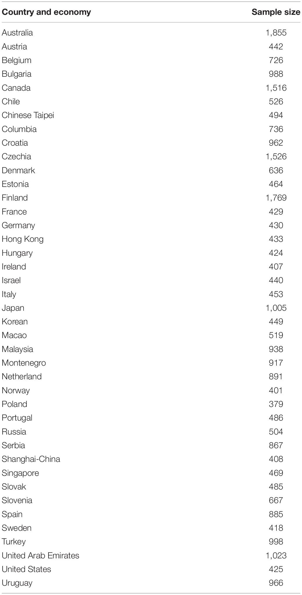
Table 1. Countries and economies with sample sizes.
This item (a snapshot of the item is shown in Figure 1) asked test takers to determine which of the three sliders controls temperature and which controls humidity, respectively. To obtain the correct answer, test takers were permitted to manipulate the sliders and monitor changes through the display. The answer to the task was given by drawing lines linking the diagrams to indicate the association between the inputs (sliders) and outputs. The correct solution is shown in Figure 1. The “reset” button undid previous simulations by clearing the display and resetting the sliders to their initial status. No limit was imposed on the number of steps of manipulation or rounds of exploration. Also, no time constraint was imposed on each item; however, the total test time of a test cluster (problem-solving items) was limited to 20 min. Either one or two clusters were randomly given to a participant depending on different assessment designs (Organisation for Economic Co-operation and Development [OECD], 2014b). The order of items in a cluster was fixed, and a former item could not be resumed once the next item had begun. According to different assignments of clusters, the position of Climate Control Task 1 varied across test forms. For this item, the average time spent by students was 125.5 s and the median time was 114.5 s; 95% of examinees spent from 22.2 s to 290.2 s on the item; only 1,149 participants (about 3.8% of the total sample) finished the task in 30 s or less, with a 5.1% rate of correctness. Given these results, later sections of the paper assume that the item is not considered as speeded for this sample in general and position effects, if any, are negligible. However, the analysis of the current study conducted without considering the speeded issue which should be noted as a limitation and further investigated by future research.
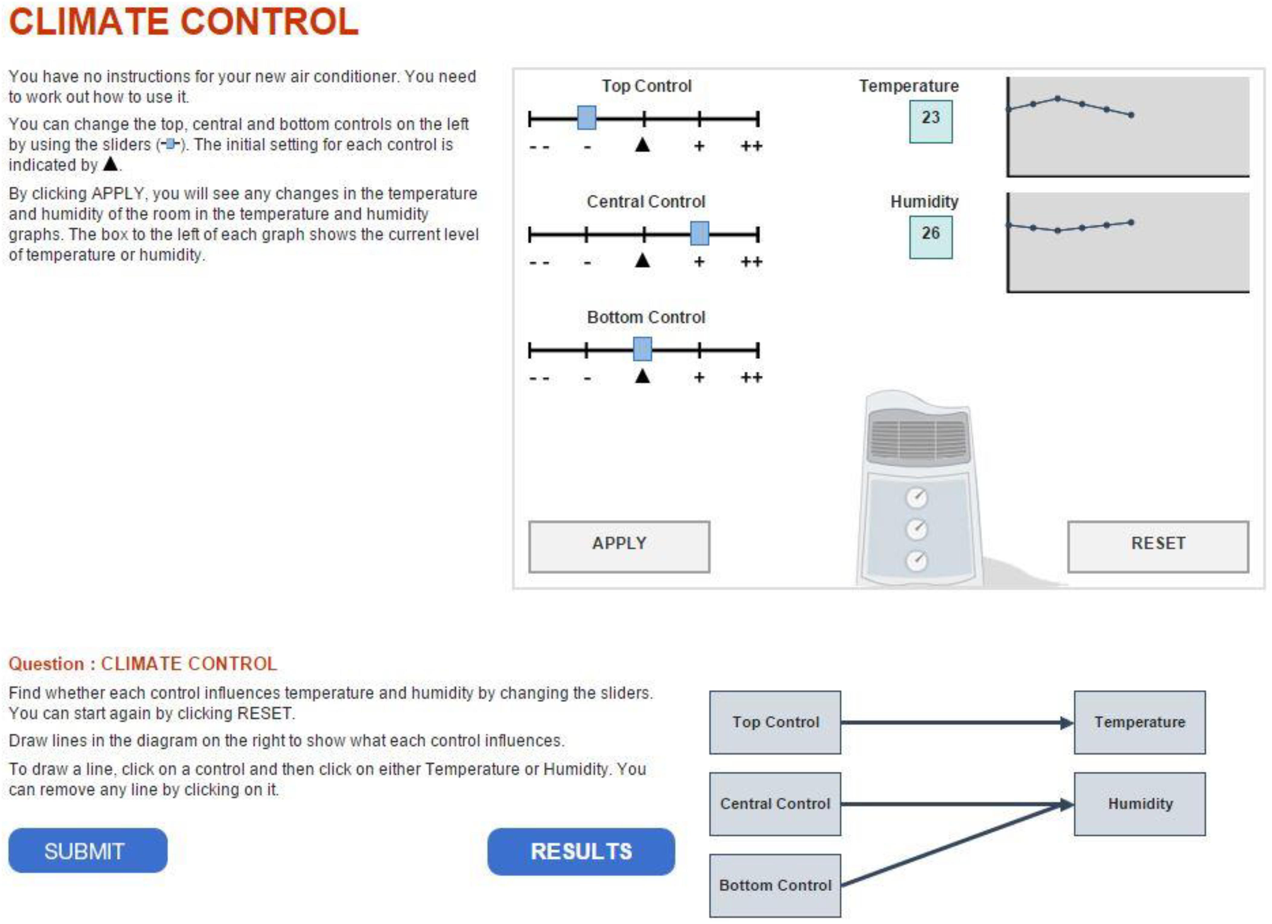
Figure 1. A snapshot of the problem-solving item Climate Control in PISA 2012.
Items like Climate Control Task 1 are constructed using the MicroDYN approach (Greiff et al., 2012) that combines the use of the theoretical framework of linear structural equation models to systematically construct tasks (Funke, 2001) with multiple independent tasks to increase reliability. Briefly speaking, a system of causal relations (e.g., the first slider controls temperature) is embedded in a scenario that allows participants to explore input variables and observe the corresponding changes of output variables through a graphical representation. No specific prior domain knowledge is required for this type of task in general. However, examinees need to gain and have command of the knowledge by exploring and experimenting before providing appropriate answers. For such tasks, a strategic knowledge for effective exploration is crucially important (Greiff et al., 2015)—that is, the VOTAT (vary one thing at a time; Tschirgi, 1980) strategy; this term is also known as the control-of-variable strategy (Chen and Klahr, 1999) in developmental psychology.
In PISA 2012, a partial credit assignment – 0 for incorrect, 1 for partially correct, and 2 for correct – was used to score the responses of Climate Control Task 1. Partial credit was given if a student explored the simulation by using the VOTAT strategy efficiently – only varying one control at a time when trying to change the status of each control individually at least once, regardless of actions being in adjacent attempts or in a round before resetting – but failed to correctly represent the association in a diagram.
To show that the VOTAT strategy is strongly related to performance on the item, Greiff et al. (2015) restricted polytomous responses as dichotomous by treating partially correct as incorrect and then investigated the association between the dichotomous responses with the indicator of applying the VOTAT strategy efficiently alongside other covariates. Following the same settings, the present study explored the association between the binary responses and the indicator of the use of the VOTAT strategy together with other covariates created from the process data to find out (1) whether the current partial scoring rubric was still supported by the prediction model (i.e., random forests)—namely, whether the VOTAT variable was still the most associated factor with responses while interacting with other covariates – and (2) whether the rubric was still sufficient compared with the new predictor features extracted from the process data. It should be noted that the restriction of response variable may not be applicable for items that are intended to measure a construct other than the interactive complex problem-solving (Cheng and Holyoak, 1985; Funke, 2001) skills or constructed without using the MicroDYN approach.
Table 2 shows a section of the postprocessed log file—that is, a readable process dataset whose entries are actions listed in chronological order. The even number indicates the actions belong to a certain test taker. The type of action, as well as the corresponding timestamp, was recorded for each action. Among the action types, “apply” represents actions related to manipulation of sliders because, after setting sliders, a test taker needed to hit the “apply” box, as shown in Figure 1, to see the changed value of temperature and humidity displayed. The changed status of sliders was recorded in the columns “top slider,” “central slider,” and “bottom slider.” The value of status ranges from −2 to 2. Similarly, the action type “diagram” represents drawing a line to link diagrams, as shown at the bottom right of Figure 1. The six-digit binary string shown in the table was used to record the association among diagrams that has been established. For example, “100101” indicates that the top slider controls temperature, whereas the central and bottom sliders control humidity.
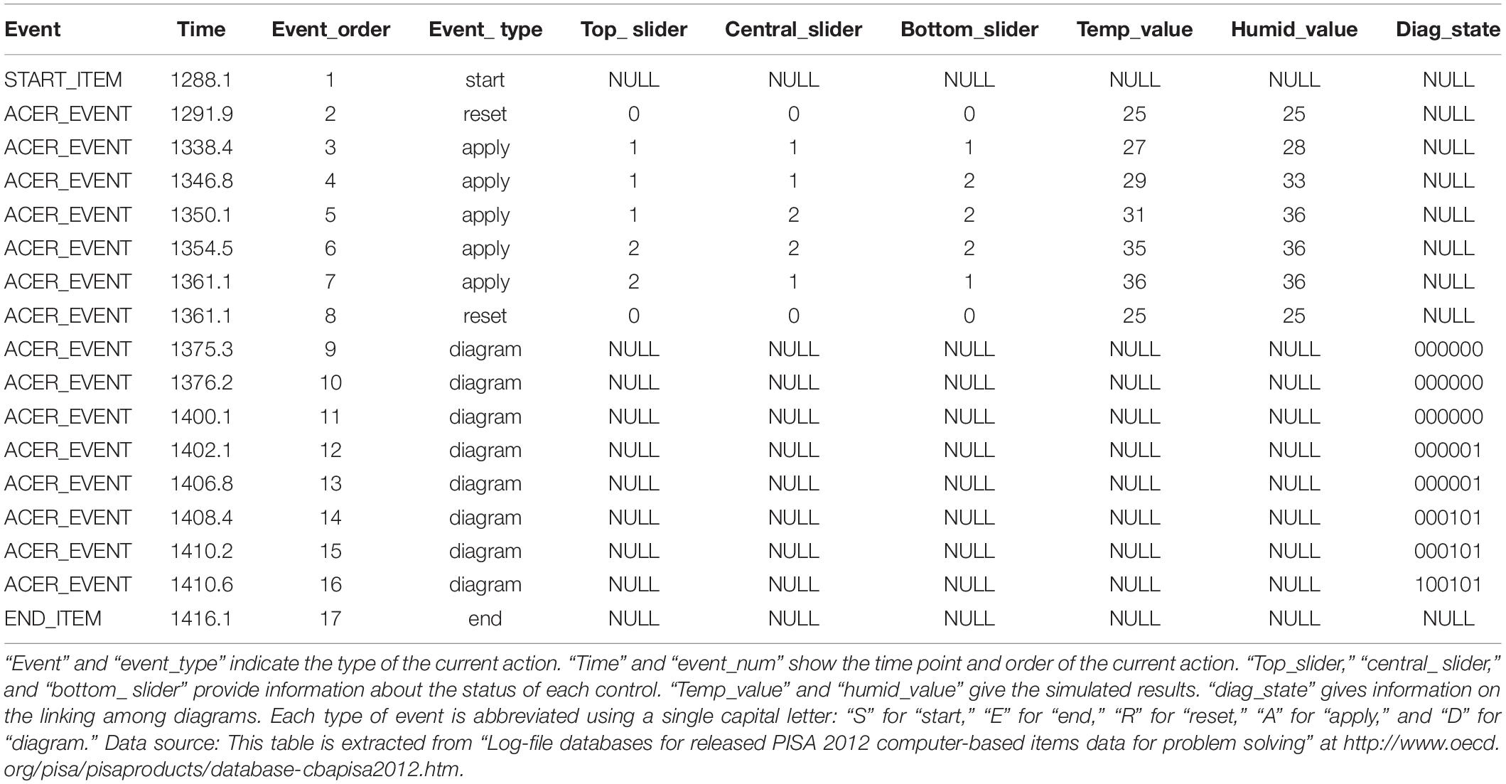
Table 2. An example of process data for a test taker solving the climate control item.
To facilitate the analysis, observed sequences of actions were collapsed into respective strings. To obtain such a string, each type of action is abbreviated using a single capital letter: “S” for “start,” “E” for “end,” “R” for “reset,” “A” for “apply,” and “D” for “diagram.” It should be noted that consecutive “D” actions were collapsed into a single “D” action because information related to drawing lines to connect the diagrams is not of central interest in the present study. For the sequence of actions shown in Table 2, it can be simplified as “SRAAAAARDE.”
Feature Generation
In this study, features (predictor variables) extracted from the process data can be summarized in three categories: variables extracted from action sequences using n-gram methods, behavior indicators, and time-related variables.
N-gram methods decode a sequence of actions into mini-sequences (e.g., a string of n letters in length where the letters remain in the same order as the original sequence of actions) and document the number of occurrences of each mini-sequence. Unigrams, analogous to the language sequences in NLP, are defined as “bags of actions,” where each single action in a sequence collection represents a distinct feature. However, unigrams are not informative in term of transitions between actions. Bigrams and trigrams are considered in this study, with action sequences broken down into mini-sequences containing two and three ordered adjacent actions. Note that the n-gram method is productive in creating features based on sequence data without loss of much information about the order of sequence. This class of methods has become widely accepted for feature engineering in fields such as NLP and genomic sequence analysis and was recently applied to analyze process data in large-scale assessment (He and von Davier, 2015, 2016). For example, an n-gram can break the action string “SRAAAAARDE” into “S(1), A(5), R(2), D(1), E(1)” for unigrams, “SA(1), AR(1), AA(4), RA(1), RD(1), DE(1)” for bigrams, and “SRA(1), RAA(1), AAA(3), AAR(1), ARD(1), RDE(1)” for trigrams, where the numerals in brackets represent the number of occurrences.
Behavior indicators can also be generated from sequences of actions. Changes to input variables (the positions of controls) shed light on participants’ problem-solving strategies and behaviors. As discussed earlier, partial credit was given to students who explored the connection between the inputs and outputs by utilizing the VOTAT (vary one thing at a time) strategy across the three controls at least once. Greiff et al. (2015) treated this scoring rubric as an indicator variable (i.e., VOTAT) and showed that it was highly associated with the probability of answering this item correctly and overall performance on the test.
This study created an ordinal categorical variable with four levels – from 0 to 3 – each number indicating on how many controls a student has used the VOTAT strategy. This ordinal variable was referred to as “VOTAT group” in the analysis. Another variable named “VOTAT num” was created to count the number of times that a student used the VOTAT strategy regardless of which control he or she applied the strategy to. Additionally, the order of “A” and “D” in a sequence of actions could convey information about examinees’ decisiveness or hesitancy of their decision-making process. For example, the action string “SRAAAAARDE” can be categorized as a meta-strategy “AD sequence,” implying the examinee “draws” the diagrams right after “applying” the simulations on sliders rather than jumping back and forth between applying sliders and drawing diagram lines.
Table 3 shows the distribution of the AD sequence variable, where N indicates the cases in which participants did not conduct an experiment or generate diagrams. Note that the AD sequence’s having an undue number of levels not just hindered interpretation but also caused data sparsity in analysis that followed. Thus a “compact” version of AD sequence with fewer levels was created as shown in Table 4. Figure 2 illustrates how to create the contracted levels in Table 4 by a tree-like diagram.
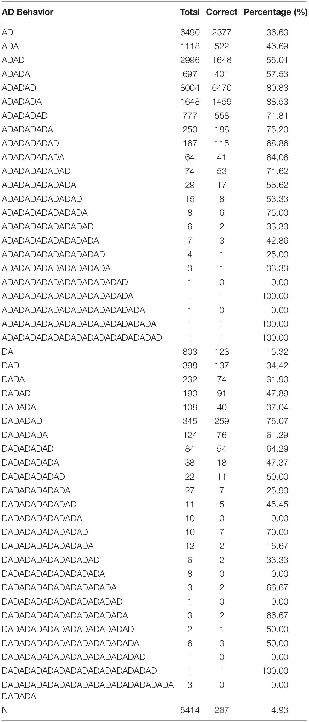
Table 3. All levels of AD sequence with sample size and percentage of correctness.
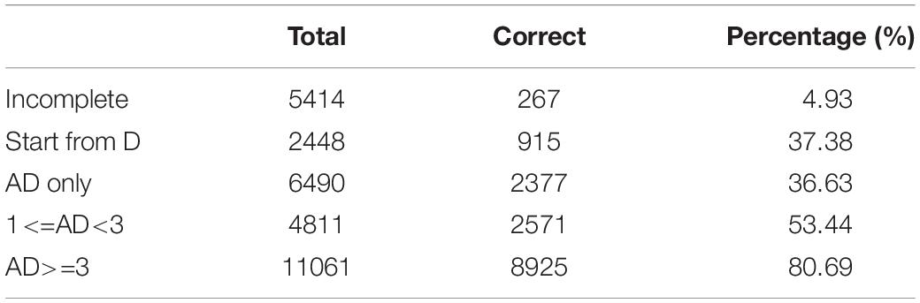
Table 4. All contracted levels of AD sequence with sample size and percentage of correctness.
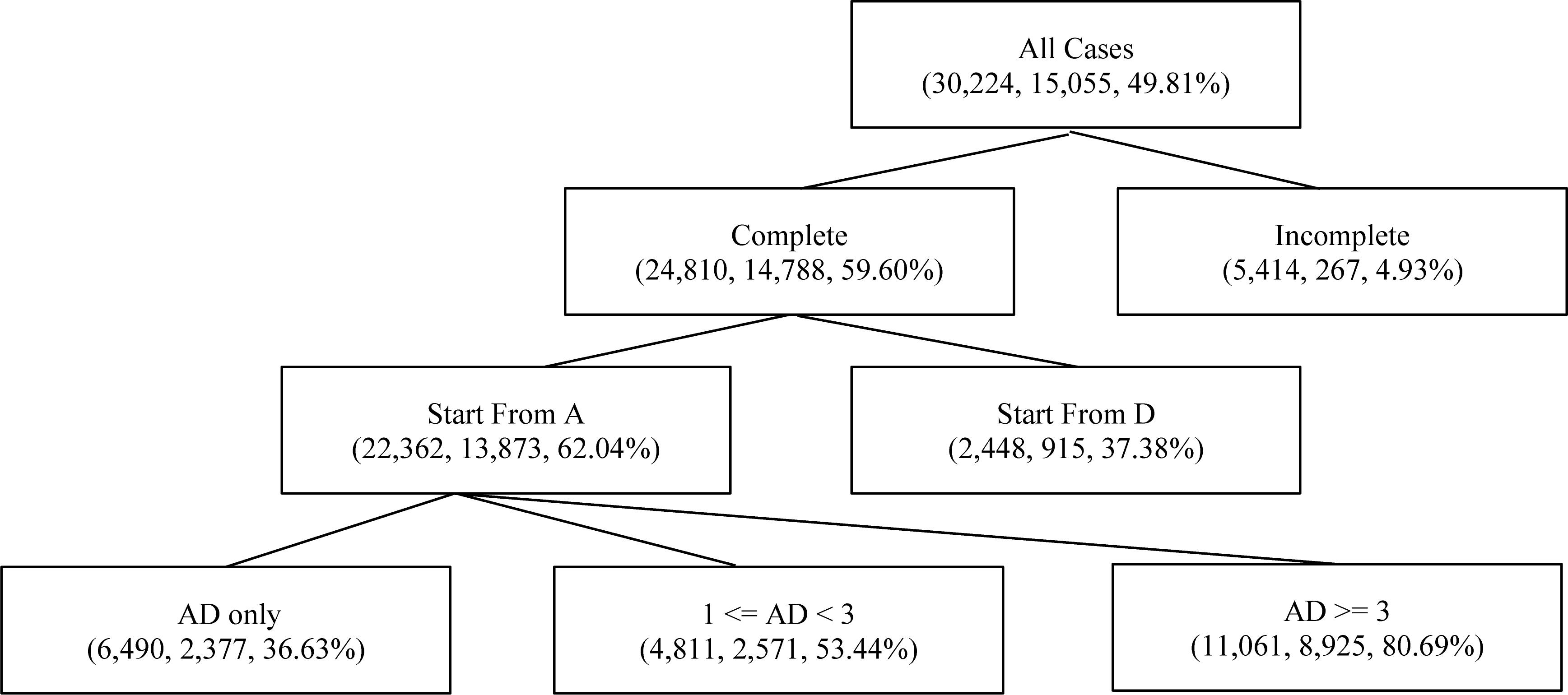
Figure 2. A tree-based diagram for contracted levels of the AD sequence. Indices in parentheses are sample size, number of correct responses, and conditional probability of correctness, respectively, for each class or contracted class of the “AD sequence” variable.
Process data also provide rich information related to time. Process data includes timestamps of actions, allowing the time spent on a specific action to be calculated by taking the difference of the time of two adjacent actions. Several time-related predictor variables can be generated as follows. “A time” and “D time” indicate the accumulated time spent on manipulating controls and drawing diagrams, respectively. For example, for an action sequence “SADRE,” “A time” is the time used after hitting the “start” box and before hitting the “apply” box; “D time” is the time spent after hitting the “apply” box and before drawing a line among diagrams. By a similar token, “E time” records the time spent after conducting the last action before hitting the “end” box. A special case is “R time,” which represents the time spent after hitting the “reset” box but before conducting the next Action. “time_bf_action” records the time span between “start” and the first action after “start,” which can be considered as the time spent on reading and perceiving the task.
Given the feature generation method described above, 77 variables were created from the process data (a snapshot of the process data is presented as Table 2), as presented in Table 5. Note that time-related features in this study were binned with equal percentiles in terms of their frequencies – the frequency of each bin ranges from 10 to 25% of the sample depending on the variables. This was done essentially due to the nature of the tree models: continuous variables are discretized to find the best “split” point, as discussed in previous sections. This inherent discretization mechanism tends to create data sparsity when the distribution of a continuous variable is “discontinued” (i.e., having extreme low density at the area between modes), which increases the chance of encountering a computation failure. Therefore, to reduce this chance, practitioners “stabilize” the distributions of these “discontinued” variables by binning before feeding the variables to fit the algorithm. In this study, binning was also applied to n-gram features with levels having sparse sample sizes. However, it should be noted that binning entails a risk of losing information about these variables.

Table 5. Variables generated from process data of climate control task 1.
Feature Selection
Feature selection was conducted using the R package randomForest (Liaw and Wiener, 2002). The selection began with seeking the random forest algorithm having the optimal complexity to fit the dataset. In this study, the complexity of the random forest algorithm is characterized by combinations of number of trees (ntree) and number of predictor variables used to grow a tree (mtry). Empirical studies (Breiman, 2001; Mitchell, 2011; Janitza and Hornung, 2018) showed that mtry and ntree are more influential than other factors in controlling the complexity of the random forest algorithm. In this study the size of a tree (i.e., the number of generations or the total number of nodes) was not restricted and the number of branches used at each split was fixed at 2. The present study was focused on exploring the combinations of mtry and ntree, where ntree = 100, 300, 500, and mtry = 4, 6, 8, 10, 12.
Cross-Validation
A typical way to find the optimal model complexity (i.e., the combination of tuning parameters) is to compare the fitted models by their validation error. The validation error is obtained by holding out a subset of the sample (validation set), using the retained sample (training set) to fit the classification algorithm, and then estimating the prediction error by applying the fitted algorithm to the validation set. To efficiently utilize data with a limited size, practitioners (Breiman and Spector, 1992; Kohavi, 1995) have recommended five- or ten-fold cross-validation. In the case of five-fold cross-validation, the data is split into five roughly equal parts. A loop of validations is then conducted – each part is labeled as the validation set once to estimate the prediction error of the random forest model fitted using the other four parts. In a data-rich situation, Hastie et al. (2009) recommended to isolate an additional set (the test set) from the sample before conducting cross-validation. This set is used to compute the prediction error for the final chosen model. It can also be considered as an assessment of the generalization performance of the chosen model on independent data. The present study randomly selected roughly 10% of the sample (3,000 students) as the test set; the rest was separated into five folds for the training-validation purposes.
Variable Selection and Backward Elimination
The core idea of validation is to keep the validation sample from being “seen” by the model training process. Such a principle must also be obeyed when variable selection is involved. An example of violating this rule would be to conduct variable selection based on the whole sample before tuning model parameters based on cross-validation (Hastie et al., 2009).
The variable selection implemented in the current study is based on the recursive feature elimination in Guyon et al. (2002) that iteratively rules out features at the lower end of the ranking criterion. Together with random forests, recursive feature elimination has been successfully employed in genome-wide association studies (e.g., Jiang et al., 2009). The variable selection approach suggested in the present study is not just an application of recursive feature elimination using the random forest algorithm with a specific focus on the process data, but a modification with an emphasis on end-to-end cross-validation.
Box 1. Backward elimination algorithm for feature selection.
randomly split the training-validation dataset into 5 disjoint subsets.X1,…,X5 are sets of covariates; they are all same with 77 covariates at the beginning;
repeat the followings until the covariate sets X1, …, X5 are empty:
for k in {1,2,…,5}:
hold the k-th dataset out for ranking;
for each combination of mtry and ntree:
conduct a five-fold cross-validation using the other 4 datasets and covariates left in Xk;
obtain cross-validated prediction error e for the current combination; find the optimal mtry and ntree by comparing e across all combinations; fit a random forest using the k-th dataset and the optimal parameters; obtain the importance rank and remove the least important feature from Xk.
end
Box 1 outlines the suggested backward elimination algorithm for variable selection. Note that to prevent variable selection (i.e., ranking) from seeing the data used for model training (i.e., parameter tuning in this study), the training-validation dataset was divided into five disjoint subsets in this recursive selection process so that at each backward elimination parameter tuning can be conducted using four of the subsets of data while variable ranking can be performed separately based on the other subset. This suggested approach follows the principles of variable selection for study design recommended by Brick et al. (2017).
As indicated by Box 1, the backward elimination also documents how the validation performance of the fitted model changes as the number of features reduces, which was illustrated in Figure 3. The number of selected features was decided by drawing a cutoff line around where the first large drop in prediction performance begins (i.e., 49 in Figure 3). Setting this cutoff line here is like selecting the number of factors using the scree plot (Cattell, 1966). Given this threshold number (i.e., 77−49 = 28), five sets with 28 selected features were obtained, and their intersection gives the final selected set of features (26 features).
Figure 3. Prediction performance versus number of eliminated predictors for a backward elimination. Dashed lines record the change of validation performance (classification accuracy) for each training set as the number of eliminated feature increases; the bold solid line represents the average performance for five-fold; the vertical dashed line (the number of excluded features=49) indicates where a large reduction of prediction performance begins.
The backward elimination in Box 1 has five separated iterative variable ranking processes, which could be somehow regarded as an implicit self-validation. However, the determination of the cut-off line shared by the five ranking processes (i.e., the feature screening) should be further validated if data are rich enough. Instead of having one training-validation set, five disjointed training-validation sets (notice this is different from the five shown in Box 1) were established after the test set was held out. Backward elimination shown in Box 1 was conducted for each of the five sets. Accordingly, five sets of final selected features were obtained. Table 6 shows the intersection of these five sets of selected features.
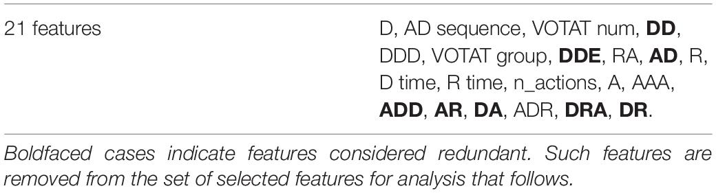
Table 6. Features selected through the five-fold validated backward elimination.
The backward elimination in Box 1 was structured using a nested loop that might cause inefficiency. Practitioners can increase the number of features eliminated for each round to reduce computation burden. Plus, as noted by Breiman (2001), the value of mtry set around the square root of the number of predictors seems to have minimal effect on validation performance; to increase computational efficiency, one can utilize this deterministic way to adapt the value of mtry. In addition, to further increase algorithmic efficiency, researchers (Breiman, 2001; Nicodemus and Malley, 2009; Zhang et al., 2010; Goldstein et al., 2011; Oliveira et al., 2012) recommended employing out-of-bag error as an alternative to cross-validation error. Simulation studies (Mitchell, 2011; Janitza and Hornung, 2018) showed that although out-of-bag error tends to overestimate true error rate when “n≪p”—that is, the sample size is far less than the number of predictors, the overall validation performance is not substantially affected by means of out-of-bag error to determine model complexity. The present study also performed a backward elimination boosted by using the above suggestions, which obtained consistent results with the plain approach shown in Box 1 in terms of variable selection. Such results were not presented in the manuscript for the sake of simplicity.
Results
The final set of selected features includes ordinal and binary categorical variables. Pairwise associations among these ordinal variables were measured using the Goodman-Kruskal gamma (γ; Goodman and Kruskal, 1954) with value from −1 (discordant) to 1 (concordant). Given the measure, the final set can be further reduced by removing the redundant features highly related to others.
Among all pairs, “DD” was highly associated with “DDD”(γ = 0.76); “AR” and “RA” was associated with γ = 0.71; other well-associated pairs (γ > 0.6) included “AD sequence” with “AD,” “AD sequence” with “DA,” “AD” with “ADD,” “DRA” with “ADR,” “DRA” with “DR,” and “DD” with “DDE.”3 It is not surprising that “AD sequence” was highly correlated with “AD” and “DA.” “AD sequence” was preferred since it covered more information than “AD” and “DA” do, as discussed earlier. “DDD” was greatly associated with “DD;” trigram was preferable in this case since it contained more detailed information. “DDE” conveyed trivial information compared to “DD” and “DDD,” as did “ADD” to “AD.” “AR” and “RA” covered similar information, as did “DRA” with “DR” and “ADR;” the one with higher rank of permutation importance was preferred. In sum, eight features (boldfaced in Table 6) were excluded: “AD,” “DA,” “ADD,” “DDE,” “DRA,” “AR,” “DD,” and “DR.”
With the 13 remaining features, a random forest was fitted with the parameter set where ntree = 100 and mtry = 4. The parameter combination was chosen based on validation performance of the test set that had been held out at the beginning. Applying the test set here was necessary since the association measured above was based on the entire validation-training sample, which means that variables selected using γ had already “seen” the validation data. Similarly, another random forest was fitted with 77 features; the parameter set was tuned using the test data, where ntree = 300 and mtry = 9. Here the Goodman-Kruskal tau (τ; Goodman and Kruskal, 1954) was used to measure the proportional reduction of incorrect prediction for the full and the reduced model, respectively, with regard to the random guess based on observed distribution of responses, where τ77 = 0.810 and τ13 = 0.797. In this regard, the reduced model performed decently in comparison to the full model.
Features of the simple model ranked by the permutation importance measure are shown in Table 7. Unigram “D,” “R,” and “A” ranked high in the list since they are basic elements constituting action sequences. Furthermore, “D” and “R” are not just fundamental but also imply a student’s decisiveness. Using only a few necessary steps of drawing arrows or applying the reset function only a limited number of times might indicate confidence in providing a correct solution. “VOTAT group” and “VOTAT num” are both critical as shown in the list, which is consistent with the results found by Greiff et al. (2015). The top-ranked “AD sequence” indicates that contracting levels shown in Figure 2 work fine in summarizing students’ behaviors on experimenting. Grams such as “AAA,” “ADR,” and “RA” offer interesting perspectives. For instance, students having a large number of “AAA” tended to show certain patterns in their actions: drawing diagrams right after applying experiments (i.e., the level “AD only” in the feature “AD sequence”) and applying the VOTAT scheme across the three sliders. In further investigating these students, we found that they attempted to create an increasing or decreasing slope of the value of temperature or humidity in the display by repeatedly hitting the “apply” box while fixing the sliders at one particular status, indicating a relatively sophisticated behavior of solving the problem. Frequent usage of “ADR” and “RA” indicated participants utilized the reset function to assist their experimenting and exploration on inputs. “D time” and “R time” can be regarded as time spent on deliberation.
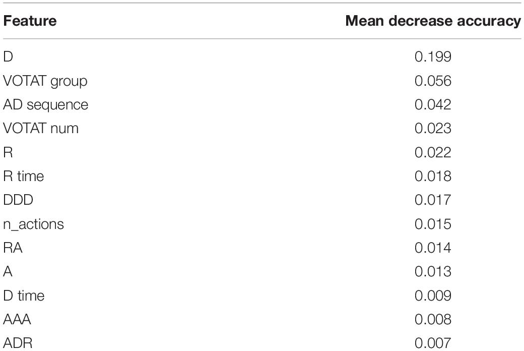
Table 7. Features ranked by permutation importance measure (mean decrease accuracy).
Discussion
The aim of the present study is to pedagogically suggest an integrated approach to analyze action sequences and other information extracted from process data. Feature generation and selection are two essential parts of the suggested approach and should be treated with equal importance. Features in this study were created following both top-down and bottom-up schemes. The former generates features based on hypotheses that might be developed by item designers and content experts. The latter, as an example, extracts features by utilizing n-gram methods and related methods breaking up the action sequences. Thus, n-gram translates the action sequences into mini-sequences along with their frequencies. Features generated by both schemes are presented in the final set of selected predictive features. The random forest algorithm was implemented in the feature selection part, which simultaneously handled (1) a massive number of categorical predictor variables, (2) the complexity of the variable structure, and (3) model/variable selection in a computationally efficient way. The utility of the suggested approach has been illustrated by implementing it in a publicly available dataset.
The suggested approach is not free from limitations. First, the feature generation process involves breaking up action sequences into mini-sequences encoded as n-grams, suggesting that the information contained in the order of the action sequences – for example, the “longer term” dependencies among actions – would not be completely preserved and exploited. As an outcome, only limited amounts of behavioral indicators are generated; information embedded in students’ action sequences might not be fully utilized. For example, the range of states of controls explored by a student is a variable likely associated with the response variable. Technically speaking, to preserve more “complete” information when analyzing action sequences, sequence-mining approaches (e.g., SPADE; Zaki, 2001) employed to find common subsequences provide a possible alternative. Also, ideas stemming from cognitive and learning studies offer a theoretical basis of creating features from action sequences; for example, some studies (Jiang et al., 2015, 2018) employed sequential pattern mining to analyze learning skills and performance in immersive virtual environments.
Second, most features, if not all, are ordinal categorical variables representing frequency. As noted in the previous section, some variables present in excessive levels could cause an issue of data sparsity when conducting the random forest algorithm. This study used equal-percentile binning to address this issue at the expense of losing information provided by the original variables. The sensitivity of binning needs to be further investigated.
Third, the CART-based random forest algorithm using the Gini-impurity index to split nodes (e.g., the randomForest R package used in this study) implemented in this study is generally a suboptimal choice. Strobl et al. (2007) showed that the algorithm tends to favor categorical variables with extensive levels as well as a cluster of variables that are highly correlated. The modified random forest algorithm proposed by Strobl et al. (2007) using the conditional inference tree introduced by Hothorn et al. (2006) should be explored in the context of process data for future studies.
Fourth, even though the efficiency of the suggested backward elimination can be increased by using several steps noted in the previous section, the computation burden is still a concern for the present study. Backward elimination with the specifications shown in Box 1 was validated using a five-fold dataset, which took about 19,872 s in total on a Mac Pro desktop with a 3.5 GHz CPU and 16 GB of RAM.
Fifth, like other data-driven algorithms, the random forest approach is not straightforward regarding model interpretation. For example, hypothesis tests on marginal effects of features are not sustained in random forests; the directions of marginal effects are not directly accessible, either. Friedman (2001) suggested plotting the partial dependence between the feature and the outcome variable (logit is used if the outcome variable is categorical) to access the marginal effects. This display method has been implemented in the R package randomForest as the function partialPlot. It is sensible to apply models with more restricted functional forms, such as linear models, to conduct an ad hoc analysis based on the selected features.
Sixth, the random forest algorithm is a data-driven method that is sensitive to sample characteristics. Meanwhile, PISA is an international large-scale assessment involving mixed-type forms of tests and multistage sampling designs. The question on how the sampling designs affect the analysis using data-driven methods (i.e., random forests) in terms of estimation stability is beyond the scope of this study. It is appealing that future methodological research could provide guidance concerning the correct use of cross-validation in different test designs.
Last, the exploratory nature of the suggested approach comes with the purpose of the study. Although interesting patterns of behaviors have been found by the suggested approach, it is still difficult to test a cognitive or psychometric theory with it.
The suggested method offers an alternative to the generation and selection of informative features from a massive amount of process data, given the increasing attention to exploring the usage of process data along with response data in large-scale assessments. Generalizability of the method can be explored by applying it to multiple tasks constructed using a similar approach such as MicroDYN and comparing it with other variable-selection approaches in terms of practical significance.
Ethics Statement
This study is a secondary analysis based on released datasets from PISA 2012 log data files (http://www.oecd.org/pisa/pisaproducts/database-cbapisa2012.htm). No additional data were collected from human subjects for this particular study.
Author Contributions
ZH contributed to the development of methodology exploration, model estimation procedures, conduction of the data analysis, and drafting and revision of the manuscript. QH contributed to the development of the methodological framework, supervision on the model estimation procedures, conduction of the data analysis, and drafting and revision of the manuscript. MD contributed to providing suggestions on the methodological framework and the model estimation procedures, and reviewing and revision of the manuscript.
Funding
This study was partially supported by the Internship Program under Educational Testing Service and the National Science Foundation (NSF – Award #1633353).
Conflict of Interest
The authors declare that the research was conducted in the absence of any commercial or financial relationships that could be construed as a potential conflict of interest.
Acknowledgments
The authors would like to thank Larry Hanover for his help in editing the manuscript and Dr. Xiang Liu for his valuable suggestions.
Footnotes
- ^ Predictor variables and covariates are also used interchangeably without being specifically mentioned in sections that follow.
- ^ The dataset is available at http://www.oecd.org/pisa/data/pisa2012database-downloadabledata.htm.
- ^ As a reminder, “D” refers to drawing the diagram, “A” to applying the simulations on the slider, “S” to start, and “R” to reset.
References
Agrawal, R., and Srikant, R. (1995). “Mining sequential patterns,” in Proceedings of the Eleventh IEEE International Conference on Data Engineering, Taipei.
Amershi, S., and Conati, C. (2009). Combining unsupervised and supervised classification to build user models for exploratory learning environments. J. Educ. Data Min. 1, 18–81.
Anderson, E., Gulwani, S., and Popovic, Z. (2013). “A trace-based framework for analyzing and synthesizing educational progressions,” in Proceedings of the Special Interest Group on Computer-Human Interaction (SIGCHI) Conference on Human Factors in Computing Systems, (Paris).
Azevedo, R. (2005). Using hypermedia as a metacognitive tool for enhancing student learning? The role of self-regulated learning. Educ. Psychol. 40, 199–209.
Baker, R., and Yacef, K. (2009). The state of educational data mining in 2009: a review and future visions. J. Educ. Data Min. 1, 3–16.
Biswas, G., Jeong, H., Kinnebrew, J., Sulcer, B., and Roscoe, R. (2010). Measuring self-regulated learning skills through social interactions in a teachable agent environment. Res. Pract. Technol. Enhanc. Learn. 5, 123–152. doi: 10.1142/S1793206810000839
Bouchet, F., Harley, J. M., Trevors, G. J., and Azevedo, R. (2013). Clustering and profiling students according to their interactions with an intelligent tutoring system fostering self-regulated learning. J. Educ. Data Min. 5, 104–146.
Brand-Gruwel, S., Wopereis, I., and Walraven, A. (2009). A descriptive model of information problem-solving while using internet. Comput. Educ. 53, 1207–1217. doi: 10.1016/j.compedu.2009.06.004
Breiman, L., Friedman, J. H., Olshen, R. A., and Stone, C. I. (1984). Classification and regression trees. Belmont, CA: Wadsworth.
Breiman, L., and Spector, P. (1992). Submodel selection and evaluation in regression. Int. Statist. Rev. 60, 291–319.
Brick, T. R., Koffer, R. E., Gerstorf, D., and Ram, N. (2017). Feature selection methods for optimal design of studies for developmental inquiry. J. Gerontol. Ser. B Psychol. Sci. Soc. Sci. 73, 113–123. doi: 10.1093/geronb/gbx008
Cattell, R. B. (1966). The scree test for the number of factors. Multivariate Behav. Res. 1, 245–276. doi: 10.1207/s15327906mbr0102-10
Chen, Z., and Klahr, D. (1999). All other things being equal: acquisition and transfer of the control of variables strategy. Child Dev. 70, 1098–1120.
Cheng, P. W., and Holyoak, K. J. (1985). Pragmatic reasoning schemas. Cogn. Psychol. 17, 391–416. doi: 10.1016/0010-0285(85)90014-3
Chipman, H. A., George, E. I., and McCulloch, R. E. (2010). BART: bayesian additive regression trees. Ann. Appl. Statist. 4, 266–298. doi: 10.1214/09-AOAS285
Corbett, A. T., and Anderson, J. R. (1995). Knowledge tracing: modeling the acquisition of procedural knowledge. User Model. User Adapt. Interact. 4, 253–278. doi: 10.1007/BF01099821
DeMars, C. E. (2007). Changes in rapid-guessing behavior over a series of assessments. Educ. Assess. 12, 23–45. doi: 10.1080/10627190709336946
Díaz-Uriarte, R., and Alvarez de Andrés, S. (2006). Gene selection and classification of microarray data using random forest. BMC Bioinform. 7:3. doi: 10.1186/1471-2105-7-3
Dietterich, T. (2000). Ensemble methods in machine learning. Proc. Mult. Classif. Syst. 1857, 1–15. doi: 10.1007/3-540-45014-9-1
Efron, B. (1978). Regression and ANOVA with zero-one data: measures of residual variation. J. Am. Statist. Assoc. 73, 113–121. doi: 10.2307/2286531
Fink, G. A. (2008). Markov Models for Pattern Recognition. Berlin: Springer, doi: 10.1007/978-3-540-71770-6
Forman, G. (2003). An extensive empirical study of feature selection metrics for text classification. J. Mach. Learn. Res. 3, 1289–1305.
Freund, Y., and Schapire, R. E. (1997). A decision-theoretic generalization of on-line learning and an application to boosting. J. Comput. Syst. Sci. 55, 119–139. doi: 10.1006/jcss.1997.1504
Friedman, J. H. (2001). Greedy function approximation: a gradient boosting machine. Ann. Statist. 29, 1189–1232.
Funke, J. (2001). Dynamic systems as tools for analysing human judgement. Think. Reason. 7, 69–89. doi: 10.1080/13546780042000046
Gilula, Z., and Haberman, S. J. (1995). Dispersion of categorical variables and penalty functions: derivation, estimation, and comparability. J. Am. Statist. Assoc. 90, 1447–1452. doi: 10.1007/s11336-004-1175-8
Goldhammer, F., Naumann, J., and Keβel, Y. (2013). Assessing individual differences in basic computer skills: psychometric characteristics of an interactive performance measure. Eur. J. Psychol. Assess. 29, 263–275. doi: 10.1027/1015-5759/a000153
Goldhammer, F., Naumann, J., Selter, A., Toth, K., Rolke, H., and Klieme, E. (2014). The time on task effect in reading and problem-solving is moderated by task difficulty and skill: insights from a computer-based large-scale assessment. J. Educ. Psychol. 106, 608–626. doi: 10.1037/a0034716
Goldstein, B., Polley, E., and Briggs, F. (2011). Random forests for genetic association studies. Statist. Appl. Genet. Mol. Biol. 10, 1–34. doi: 10.2202/1544-6115.1691
Goodman, L., and Kruskal, W. (1954). Measures of association for cross classifications. J. Am. Statist. Assoc. 49, 732–764. doi: 10.2307/2281536
Greiff, S., Wustenberg, S., and Avvisati, F. (2015). Computer-generated log-file analyses as a window into students’ minds? A showcase study based on the PISA 2012 assessment of problem-solving. Comput. Educ. 91, 92–105. doi: 10.1016/j.compedu.2015.10.018
Greiff, S., Wüstenberg, S., and Funke, J. (2012). Dynamic problem solving: a new assessment perspective. Appl. Psychol. Measur. 36, 189–213. doi: 10.1177/0146621612439620
Guyon, I., and Elisseeff, A. (2003). An introduction to variable and feature selection. J. Mach. Learn. Res. 3, 1157–1182. doi: 10.1162/153244303322753616
Guyon, I., Weston, J., Barnhill, S., and Vapnick, V. (2002). Gene selection for cancer classification using support vector machines. Mach. Learn. 46, 389–442. doi: 10.1023/A:1012487302797
Haberman, S. J. (1982). Analysis of dispersion of multinomial responses. J. Am. Statist. Assoc. 77, 568–580. doi: 10.2307/2287713
Hao, J., Shu, Z., and Davier, A. (2015). Analyzing process data from game/scenario-based tasks: an edit distance approach. J. Educ. Data Min. 7, 33–50.
Hastie, T., Tibshirani, R., and Friedman, J. (2009). Model Assessment and Selection. The Elements of Statistical Learning. New York, NY: Springer, 219–259. doi: 10.1007/978-0-387-21606-5-7
He, Q., Borgonovi, F., and Paccagnella, M. (2019). “Using process data to understand adults’ problem-solving behaviour in the programme for the international assessment of adult competencies (PIAAC): identifying generalised patterns across multiple tasks with sequence mining,” OECD Education Working Papers (Paris: OECD Publishing). doi: 10.1787/650918f2-en
He, Q., Glas, C. A. W., Kosinski, M., Stillwell, D. J., and Veldkamp, B. P. (2014). Predicting self-monitoring skills using textual posts on Facebook. Comput. Hum. Behav. 33, 69–78. doi: 10.1016/j.chb.2013.12.026
He, Q., Veldkamp, B. P., and de Vries, T. (2012). Screening for posttraumatic stress disorder using verbal features in self-narratives: a text mining approach. Psychiatr. Res. 198, 441–447. doi: 10.1016/j.psychres.2012.01.032
He, Q., and von Davier, M. (2015). “Identifying feature sequences from process data in problem-solving items with n-grams,” in Quantitative Psychology Research: Proceedings of the 79th Annual Meeting of the Psychometric Society, eds A. van der Ark, D. Bolt, S. Chow, J. Douglas, and W. Wang (New York, NY: Springer), 173–190.
He, Q., and von Davier, M. (2016). “Analyzing process data from problem-solving items with n-grams: Insights from a computer-based large-scale assessment,” in Handbook of Research on Technology Tools For Real-World Skill Development, eds Y. Rosen, S. Ferrara, and M. Mosharraf (Hershey, PA: Information Science Reference), 749–776.
He, Q., von Davier, M., and Han, Z. (2018). “Exploring process data in computer-based international large-scale assessments,” in Data Analytics and Psychometrics: Informing Assessment Practices, eds H. Jiao, R. Lissitz, and A. van Wie (Charlotte, NC: Information Age Publishing).
Hothorn, T., Hornik, K., and Zeileis, A. (2006). Unbiased recursive partitioning: a conditional inference framework. J. Comput. Graph. Statist. 15, 651–674. doi: 10.1198/106186006X133933
Janitza, S., and Hornung, R. (2018). On the overestimation of random forest’s out-of-bag error. PLoS One 13:e0201904. doi: 10.1371/journal.pone.0201904
Jiang, R., Tang, W., Wu, X., and Fu, W. (2009). A random forest approach to the detection of epistatic interactions in case-control studies. BMC Bioinform. 10:S65. doi: 10.1186/1471-2105-10-S1-S65
Jiang, Y., Clarke-Midura, J., Baker, R. S., Paquette, L., and Keller, B. (2018). “How immersive virtual environments foster self-regulated learning,” in Digital Technologies and Instructional Design For Personalized Learning, ed. R. Zheng (Hershey, PA: IGI Global.).
Jiang, Y., Paquette, L., Baker, R. S., and Clarke-Midura, J. (2015). “Comparing novice and experienced students in virtual performance assessments,” in Proceedings of the 8th International Conference on Educational Data Mining, Madrid.
Kim, H., and Loh, W. (2001). Classification trees with unbiased multiway splits. J. Am. Statist. Assoc. 96, 589–604. doi: 10.1198/016214501753168271
Kinnebrew, J. S., Mack, D. L., and Biswas, G. (2013). “Mining temporally-interesting learning behavior patterns,” in Proceedings of the 6th International Conference on Educational Data Mining. Los Altos, CA.
Klieme, E. (2004). “Assessment of cross-curricular problem-solving competencies,” in Comparing Learning Outcomes: International Assessments and Education Policy, eds J. H. Moskowitz, and M. Stephens (London: Routledge).
Kohavi, R. (1995). A study of Cross-Validation and Bootstrap for Accuracy Estimation and Model Selection. Los Altos, CA: Morgan Kaufmann.
Kohavi, R., and John, G. (1997). Wrappers for feature selection. Artif. Intelligence 97, 273–324. doi: 10.1016/S0004-3702(97)00043-X
Lazonder, A. W., and Rouet, J. F. (2008). Information problem-solving instruction: some cognitive and metacognitive issues. Comput. Hum. Behav. 24, 753–765. doi: 10.1016/j.chb.2007.01.025
Lee, Y. H., and Haberman, S. J. (2016). Investigating test-taking behaviors using timing and process data. Int. J. Test. 16, 240–267. doi: 10.1080/15305058.2015.1085385
Liao, D., He, Q., and Jiao, H. (2019). Mapping background variables with sequential patterns in problem-solving environments: an investigation of U.S. adults’ employment status in PIAAC. Front. Psychol. 10:646. doi: 10.3389/fpsyg.2019.00646
Light, R., and Margolin, B. (1971). An analysis of variance for categorical data. J. Am. Statist. Assoc. 66, 534–544. doi: 10.2307/2283520
Lin, Y., and Jeon, Y. (2006). Random forests and adaptive nearest neighbors. J. Am. Statist. Assoc. 101, 578–590. doi: 10.1198/016214505000001230
Manning, C. D., and Schütze, H. (1999). Foundations of Statistical Natural Language Processing. Cambridge, MA: MIT Press.
Martinez, R., Yacef, K., Kay, J., Al-Qaraghuli, A., and Kharrufa, A. (2011). “Analysing frequent sequential patterns of collaborative learning activity around an interactive tabletop,” in Proceedings of the 4th International Conference on Educational Data Mining, Seattle, WA.
Mayer, R. E. (1994). “Problem-solving, teaching and testing,” in The International Encyclopedia of Education, eds T. Husen, and T. N. Postlethwaite (Oxford: Pergamon Press).
Mislevy, R. J., Behrens, J. T., Dicerbo, K. E., and Levy, R. (2012). Design and discovery in educational assessment: evidence-centered design, psychometrics, and educational data mining. J. Educ. Data Min. 4, 11–48.
Mitchell, M. (2011). Bias of the random forest out-of-bag (OOB) error for certain input parameters. Open J. Statist. 1, 205–211. doi: 10.4236/ojs.2011.13024
Nicodemus, K., and Malley, J. (2009). Predictor correlation impacts machine learning algorithms: implications for genomic studies. Bioinformatics 25, 1884–1890. doi: 10.1093/bioinformatics/btp331
Nigam, K., McCallum, A. K., Thurn, S., and Mitchell, T. (2000). Text classification from labeled and unlabeled documents using EM. Mach. Learn. 39, 103–134. doi: 10.1023/A:1007692713085
Oakes, M., Gaizauskas, R., Fowkes, H., Jonsson, W. A. V., and Beaulieu, M. (2001). “A method based on chi-square test for document classification,” in Proceedings of the 24th Annual International ACM SIGIR Conference on Research and Development in Information Retrieval, (New York, NY: ACM), 440–441. doi: 10.1145/383952.384080
Oliveira, S., Oehler, F., San-Miguel-Ayanz, J., Camia, A., and Pereira, J. (2012). Modeling spatial patterns of fire occurrence in mediterranean europe using multiple regression and random forest. Forest Ecol. Manag. 275, 117–129. doi: 10.1016/j.foreco.2012.03.003
Organisation for Economic Co-operation and Development [OECD], (2014a). PISA 2012 Results: Creative Problem-Solving: Students’ Skills in Tackling Real-Life Problems. Paris: OECD Publishing.
Organisation for Economic Co-operation and Development [OECD], (2014b). PISA 2012 Technical Report. PISA. Paris: OECD Publishing.
Peet, R. K. (1974). The measurement of species diversity. Ann. Rev. Ecol. Syst. 5, 285–307. doi: 10.1146/annurev.es.05.110174.001441
Rabiner, L. (1989). A tutorial on hidden markov models and selected applications in speech recognition. Proc. IEEE 77, 257–286. doi: 10.1109/5.18626
Ramalingam, D., McCrae, B., and Philpot, R. (2014). “The PISA assessment of problem solving,” in The Nature of Problem Solving, eds B. Csapó, and J. Funke (Paris: OECD Publishing), doi: 10.1787/9789264273955-en
Sandri, M., and Zuccolotto, P. (2008). A bias correction algorithm for the Gini variable importance measure in classification trees. J. Comput. Graph. Statist. 17, 611–628. doi: 10.1198/106186008X344522
Shannon, C. E. (1948). A mathematical theory of communication. Bell Syst. Tech. J. 27, 379–423. doi: 10.1002/j.1538-7305.1948.tb01338.x
Shapiro, A. M., and Niederhauser, D. (2004). “Learning from hypertext: research issues and findings,” in Handbook of Research on Educational Communications and Technology, ed. D. H. Jonassen (Mahwah, NJ: Lawrence Erlbaum).
Sireci, S., and Zenisky, A. (2006). “Innovative item formats in computer-based testing: In pursuit of improved construct representation,” in Handbook of Test Development, eds S. Downing, and T. Haladyna (Mahwah, NJ: Lawrence Erlbaum), doi: 10.4324/9780203874776.ch14
Strobl, C., Boulesteix, A., Zeileis, A., and Hothorn, T. (2007). Bias in random forest variable importance measure: illustrations, sources, and a solution. BMC Bioinform. 8:25. doi: 10.1186/1471-2105-8-25
Sukkarieh, J. Z., von Davier, M., and Yamamoto, K. (2012). From Biology to EDUCATION: SCORINg and Clustering Multilingual Text Sequences and Other Sequential Tasks. Princeton, NJ: Educational Testing Service.
Theil, H. (1970). On the estimation of relationships involving qualitative variables. Am. J. Sociol. 76, 103–154. doi: 10.1086/224909
Tschirgi, J. E. (1980). Sensible reasoning: a hypothesis about hypotheses. Child Dev. 51, 1–10. doi: 10.2307/1129583
van der Linden, W. (2005). Linear Models for Optimal Test Design. New York, NY: Springer, doi: 10.1007/0-387-29054-0
van der Linden, W. J., Klein Entink, R. H., and Fox, J.-P. (2010). IRT parameter estimation with response times as collateral information. Appl. Psychol. Measur. 34, 327–347. doi: 10.1177/0146621609349800
Weeks, J. P., von Davier, M., and Yamamoto, K. (2016). Using response time data to inform the coding of omitted responses. Psychol. Test Assess. Model. 58, 671–701.
White, A. P., and Liu, W. Z. (1994). Bias in information-based measures in decision tree induction. Mach. Learn. 15, 321–329. doi: 10.1007/BF00993349
Winne, P. H., and Baker, R. (2013). The potentials of educational data mining for researching metacognition, motivation and self-regulated learning. J. Educ. Data Min. 5, 1–8.
Zaki, M. J. (2001). SPADE: an efficient algorithm for mining frequent sequences. Mach. Learn. 42, 31–60. doi: 10.1023/A:1007652502315
Zhang, G., Zhang, C., and Zhang, J. (2010). Out-of-bag estimation of the optimal hyper-parameter in SubBag ensemble method. Commun. Statist. Simul. Comput. 39, 1877–1892. doi: 10.1080/03610918.2010.521277
Zhou, M., Xu, Y., Nesbit, J. C., and Winne, P. H. (2010). “Sequential pattern analysis of learning logs: methodology and applications,” in Handbook of Educational Data Mining, eds C. Romero, S. Ventura, M. Pechenizkiy, and S. J. D. Baker (Cogent OA: Taylor & Francis), 107–121. doi: 10.1201/b10274-14
Keywords: process data, interactive items, feature generation, feature selection, random forests, problem-solving, PISA
Citation: Han Z, He Q and von Davier M (2019) Predictive Feature Generation and Selection Using Process Data From PISA Interactive Problem-Solving Items: An Application of Random Forests. Front. Psychol. 10:2461. doi: 10.3389/fpsyg.2019.02461
Received: 11 January 2019; Accepted: 17 October 2019;
Published: 21 November 2019.
Edited by:
Samuel Greiff, University of Luxembourg, LuxembourgReviewed by:
Timothy R. Brick, Pennsylvania State University, United StatesDaniel W. Heck, University of Marburg, Germany
Copyright © 2019 Han, He and von Davier. This is an open-access article distributed under the terms of the Creative Commons Attribution License (CC BY). The use, distribution or reproduction in other forums is permitted, provided the original author(s) and the copyright owner(s) are credited and that the original publication in this journal is cited, in accordance with accepted academic practice. No use, distribution or reproduction is permitted which does not comply with these terms.
*Correspondence: Zhuangzhuang Han, emgyMTk4QHRjLmNvbHVtYmlhLmVkdQ==; Qiwei He, cWhlQGV0cy5vcmc=; Matthias von Davier, TXZvbkRhdmllckBuYm1lLm9yZw==