 Fang Bai
 Ding Hong
 Yingying Lu
 Huanxiang Liu
 Cunlu Xu
 Xiaojun Yao
- 1School of Pharmacy, Lanzhou University, Lanzhou, China
- 2School of Information Science and Engineering, Lanzhou University, Lanzhou, China
- 3State Key Laboratory of Applied Organic Chemistry, Department of Chemistry, Lanzhou University, Lanzhou, China
The antioxidant response elements (AREs) play a significant role in occurrence of oxidative stress and may cause multitudinous toxicity effects in the pathogenesis of a variety of diseases. Determining if one compound can activate AREs is crucial for the assessment of potential risk of compound. Here, a series of predictive models by applying multiple deep learning algorithms including deep neural networks (DNN), convolution neural networks (CNN), recurrent neural networks (RNN), and highway networks (HN) were constructed and validated based on Tox21 challenge dataset and applied to predict whether the compounds are the activators or inactivators of AREs. The built models were evaluated by various of statistical parameters, such as sensitivity, specificity, accuracy, Matthews correlation coefficient (MCC) and receiver operating characteristic (ROC) curve. The DNN prediction model based on fingerprint features has best prediction ability, with accuracy of 0.992, 0.914, and 0.917 for the training set, test set, and validation set, respectively. Consequently, these robust models can be adopted to predict the ARE response of molecules fast and accurately, which is of great significance for the evaluation of safety of compounds in the process of drug discovery and development.
Introduction
Antioxidant response elements (AREs), a series of momentous regulators of redox homeostasis and activators of cytoprotection during oxidative stress, can be activated by the exogenous sources of oxidative stress to participate in a variety of diseases ranging from cancer to neurodegeneration diseases (Raghunath et al., 2018). AREs are crucial in a variety of physiological functions and interact with numerous transcription factors to arrange the expression of a batch of cytoprotective genes in a spatio-temporal manner (Ney et al., 1990). More specifically, AREs profoundly contribute to the pathogenesis and progression of carbohydrate metabolism, cognition, inflammation, iron metabolism, metastasis, reduced nicotinamide adenine dinucleotide phosphate (NADPH) regeneration, lipid metabolism, and tissue remodeling (Hayes and Dinkova-Kostova, 2014). As such, AREs are the vital targets of the signal transduction pathway in eukaryotic cells responded to oxidative stress and the prevention of potential chemical toxicity. Therefore, determining if one compound can activate AREs is crucial for the assessment of potential risk of compound.
Generally, the in vitro and in vivo evaluations of interactions between a large number of compounds and the AREs are expensive, time-consuming and labor intensive. Relatively, the in silico approaches can be used as an alternative way to predict if a compound can activate AREs with lower cost. Based on the advantages of in silico approaches, some machine learning-based methods have been proposed to predict the AREs activators in the environment (Huang et al., 2016). However, there are some problems to be solved in the development of prediction model, such as high false positive and low precision. Several model optimization strategies were also applied, such as bagging, consensus modeling, and feature selection (Drwal et al., 2015; Filip, 2015; Abdelaziz et al., 2016; Gergo, 2016; Yoshihiro, 2016). Although these strategies can be effective on some degree, the predictive performance of traditional machine learning-based methods still needs to be improved. Undoubtedly, the process of feature filtering avoids dimensional disasters, but results in the loss of relevant information. One of the most promising models for AREs' response prediction is the DeepTox developed by Mayr et al. (2016). Based on the Tox21 challenge data, they used deep neural network methods to predict AREs' response. The best model has the area under the Receiver Operating Characteristic (ROC) curve (ROC-AUC) with 0.840 and balanced accuracy with 0.677 on the validation set. Moreover, other models based on traditional machine learning methods, such as random forest (RF), support vector machine (SVM) and Naive Bayesian etc., displayed ROC-AUC ranging from 0.768 to 0.832 and the balanced accuracy ranging from 0.519 to 0.729 (Huang et al., 2016). From above all, the more reliable models for the prediction of AREs' response are still needed.
Recently, deep learning (Lecun et al., 2015), as a promising machine learning method, has been applied in a wide range of fields, such as physics, life science and medical science (Gulshan et al., 2016). There were also some researches in biology (Mamoshina et al., 2016; Dang et al., 2018; Hou et al., 2018) and drug design areas (Gawehn et al., 2016; Hughes and Swamidass, 2017). Furthermore, deep learning methods have been also applied in small molecule toxicity assessment (Blomme and Will, 2016). For example, deep neural networks (DNN) was applied to predict drug-induced liver injury (Xu et al., 2015; Fraser et al., 2018). Convolution neural networks (CNN) was applied to predict the acute oral toxicity (Xu et al., 2017). Relative to other machine learning methods, deep learning methods (Wu and Wei, 2018) have some special advantages. For example, deep learning does not require feature selection, which can make the maximum use of extracted molecular features. Secondly, deep learning integrates a multi-layered network that enables the integration and selective activation of molecular features to avoid overfitting problems. Thirdly, deep learning includes many different network structures and can analyze and classify the problems from different perspectives. All of these suggests that the emerging deep learning algorithms may help us build more reliable models to predict AREs' response of the studied compounds.
In this study, to build more reliable prediction model of AREs' response, a series of deep learning methods including deep neural networks (DNN), recurrent neural network (RNN), highway networks (HN), convolution neural networks (CNN) were applied on a large date set (Tox21 challenge data) including 8,630 compounds. For comparison, the traditional machine learning methods, random forest (RF) and support vector machine (SVM), were also applied to predict AREs' response.
Materials and Methods
Data Collection and Preparation
Tox21 challenge data1 (shown in Supporting Information) was used to build model. The structures of compounds was downloaded from PubChem2 according to the SID of compound. The AREs' response of compound was detected by CellSensor ARE-bla HepG2 cell line (Invitrogen), which was widely used to analyze the Nrf2/antioxidant response signaling pathway. To get the reliable data, each compound was tested in parallel by measuring the cell viability using CellTiter-Glo assay (Promega, Madison, WI) in the same wells. According to the test results, the molecules were categorized as “active,” “inactive,” or “inconclusion.” To keep the built models reliable, the molecules with label of “inconclusion” were removed. The three-dimensional conformations of molecules play a pivotal role in the development of prediction model (Foloppe and Chen, 2009). Therefore, all compounds used in this study were initially subjected to full geometry optimization in LigPrep (Schrödinger, 2015). During the geometry optimization, the energy minimization was carried out using OPLS2005 force field (Kaminski et al., 2001). The inorganic compounds, mixtures, counterions, tautomers, and the duplicates were removed to make sure each compound has only one optimized conformation. The ionizable groups were taken into consideration and the distinct conformations were produced with the pH window of 7.0 ± 0.2. In particular, the molecules were deleted if there were some unreasonable or improper structures. After these pretreatments, the remaining compounds include 1,136 active and 6,299 inactive compounds.
Molecular Representation
The conventional molecular descriptors and molecular fingerprint features calculated by DRAGON 7.0 software (Kode srl, 2017) were used to describe the structural features of studied compounds. The calculated molecular descriptors include 0D (constitutional descriptors), 1D (functional groups counts, atom-centered fragments), 2D, and 3D-descriptors. The descriptors with missing values were removed. After this procedure, the number of remained molecular descriptors was 5,024. In general, the chemical features shared with those most active samples would be recognized to develop prediction models in the construction phase, while other chemical features shared with the least active molecules would be removed in order to avoid the complexity and increase the efficiency of models. The most relevant descriptors correlated with ARE toxicity were selected by Gini Index3.
Molecular fingerprints (FPs) encode the structural information of a molecule by exploding its structure in all the possible substructure patterns. By this method, a molecule is described as a binary string of substructure keys. Different substructure patterns with SMARTS lists are predefined in a dictionary, within which substructures are created as atom-centered fragments using a variant of Morgan's extended connectivity algorithm. For a SMARTS pattern, if a substructure was presented in the given molecule, the corresponding bit was set to “1” and otherwise set to “0.” In this study, the 1,024 bits extended connectivity fingerprints (ECFP) (Rogers and Hahn, 2010) were calculated by the DRAGON 7.0 program (Kode srl, 2017).
Data Splitting
To build the reliable model, the representative data set should be selected to build and test model. For this aim, we divided the data set into training set, test set and validation set with the ratio of 4:1:1 by the Kennard and Stone algorithm (Kennard and Stone, 1969) by considering the structural features and activity of compound. The statistical summary of the data set was presented in Table 1. To show the distribution of compounds in training set and test set , principal component analysis (PCA)4 was performed based on the fingerprint features of compounds and the obtained results were shown in Figure 1, indicating that the compounds in training set and test set are well-distributed in the whole compound space.
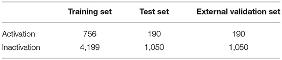
Table 1. The statistical summary of the data sets.
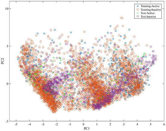
Figure 1. The distribution of samples in the training set and test set by principle component analysis (PCA) based on the molecular fingerprint features.
Machine Learning Methods
Recently, deep learning (Lecun et al., 2015) algorithms have been widely applied in a variety of areas and gave promising results (Mamoshina et al., 2016). Deep learning methods comprise a lot of architectures, such as deep neural networks (DNN), recurrent neural network (RNN), highway networks (HN), and convolution neural networks (CNN). The principle of the used deep learning methods was described as below. Due that the RF (Breiman, 2001) and SVM (Mavroforakis and Theodoridis, 2006) have been introduced elsewhere, here, their principle was not given again.
DNN Classifier
The DNNs (Lecun et al., 2015) are developed from the structure of artificial neural networks with a large number of hidden layers. In the canonical deployment, the data are fed into the input layer and then transformed in a non-linear way through multiple hidden layers, and the final results are calculated and produced to the output layer. Neurons of hidden and output layer are connected to all neurons of the previous layer's. Each neuron calculates a weighted sum of its inputs and applies a non-linear activation function to generate its output as shown in Figure 2.
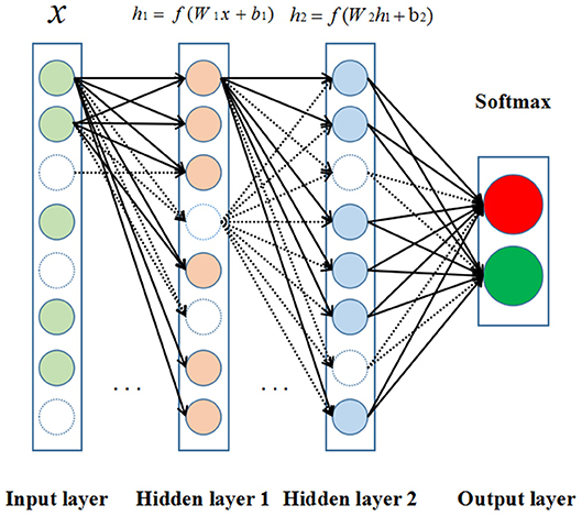
Figure 2. The structure of deep neural network (DNN). Neurons are represented by circles. The colored circles indicate the activated neurons while the circles without color are inactivated neurons. In addition, the arrows represent heavy-weight transmissions between neurons, and the dashed arrows mean the invalid neuronal connections.
HN Classifier
The HNs (Srivastava et al., 2015) allows unimpeded information flow across several layers on information highways. The architecture is characterized by the use of gating units learning to regulate the flow of information through a network. HNs increases the possibility of studying extremely deep and efficient architectures for that it can be trained hundreds of layers directly with a variety of activation functions.
RNN Classifier
RNNs (Williams and Zipser, 1989) dedicates to process sequence data as it delivers state-of-the-art results in cursive handwriting and speech recognition. Its recent application in protein intrinsic disorder prediction demonstrated its significant ability to capture non-local interactions in protein sequences (Hanson et al., 2017). RNN processes an input sequence one element at a time, maintaining in its hidden units as a “state vector” that implicitly contains information about the history of all the past elements of the sequence. However, the training process becomes problematic for the backpropagated gradients either grow or shrink at each time step. After a batch of time steps they typically exploded or vanished (Hochreiter, 1991; Bengio et al., 2002). To solve the problem, a strategy was developed to augment the networks with an explicit memory-the long short-term memory (LSTM) networks. LSTM networks define special hidden units to remember the inputs for a long time (Hochreiter and Schmidhuber, 1997). A special unit called the memory cell acts like an accumulator or a gated leaky neuron. The cell has a connection to itself, so it copies its own real-valued state and it also accumulates the external signal at the same time. This self-connection mechanism decides whether to clear the content of the memory according to the other units states. LSTM networks have subsequently proved to be more effective than conventional RNNs, especially in several layers for each time step (Graves et al., 2013).
CNN Classifier
The CNNs (Krizhevsky et al., 2012) is a kind of multi-layer neural networks designed to process data fed in the form of multiple arrays. CNNs can exploit the property of many compositional hierarchies natural signals, owing to its ability of extracting higher-level features from lower-level ones. The architecture of typical CNN consists of three types of layers, which are convolutional, pooling, and fully-connected layers. Units in a convolutional layer are organized in feature maps. Each unit is connected to local patches of feature maps as well as previous layer through a set of weights called filter bank. After the process of convolutional layer, the new feature maps are obtained by applying a non-linear activation function, such as ReLU. The pooling layer is utilized to create an invariance filter to get small shifts and distortions by reducing the dimension of the feature maps. Each feature map of a pooling layer is connected to its preceding corresponding convolutional layers. The pooling layer computes the maximum of local patch of units in each feature map. And then the convolution and pooling layers are stacked by one or more fully-connected layers aiming to perform high-level reasoning feature generation (Hinton et al., 2012; Zeiler and Fergus, 2014).
The Implementations of Machine Learning Methods
For deep learning methods, the MinMaxScaler was utilized to transform features, by which each feature was scaled into a given range between zero and one. The nodes in the network used both rectified linear units (ReLUs) and tanh functions as activation functions. The dropout algorithm (Hinton et al., 2012; Dahl et al., 2014) and L2 regularization were used to prevent overfitting. The model was trained using Adam (Adaptive Moment Estimation) optimizer (Tieleman and Hinton, 2012). Xaiver initialization was applied to initialize the parameters (Glorot and Bengio, 2010; He et al., 2015). Grid search method was employed to search the best hyperparameters. It should be noted that CNN model was built based on fingerprint features but not the descriptors, for the reason that CNN could only process highly correlated local regions of input sequences (Lecun et al., 2015). The other models were constructed based on both fingerprints and descriptors. All Deep Learning methods were implemented in Deep Learning framework of Tensorflow (version 1.5.0). All deep learning methods had 3 layers and with dropout rate of 0.1. The loss function was cross entropy. The other hyperparameters of the deep learning methods are listed in Table 2. The RF and SVM proceeded in Python scikit-learn (version 0.19.0) (Pedregosa et al., 2011). There were 80 trees in RF models. For SVM models, the kernel function was set as polynomial with gamma 0.1.

Table 2. The hyperparameters of deep learning methods.
The Evaluation of Model Performance
The performance of generated models was evaluated by several statistic metrics, such as sensitivity (SE), specificity (SP), accuracy (ACC), Matthews correlation coefficient (MCC) (Fang et al., 2013), F1-score, and Precision. The formulas are shown as below:
Where TP, TN, FP, and FN refer to the numbers of true positives, true negatives, false positives, and false negatives, respectively. All these various validation requirements have been suggested to evaluate the model performance. The Receiver Operating Characteristic (ROC) curve and the area under ROC curve (ROC-AUC) were also calculated to evaluate the predictive ability of built model.
Results and Discussion
Performance Evaluation of Descriptors-Based Classification Models
In this study, firstly, we employed various algorithms to build classification models based on molecular descriptors. The statistical evaluation of these models on the training set, test set and validation set are summarized in Table 3. For clarity, we have grouped all the metrics by training, test and validation sets and presented them as radar plots. A perfect score on all metrics would be represented by a circle the size of the complete plot. The shape of the plots can also be indicative of the quality of the models. The larger the circle is, the better the model is. The radar plots of ARE toxicity model based on the structural descriptors are shown in Figure 3.
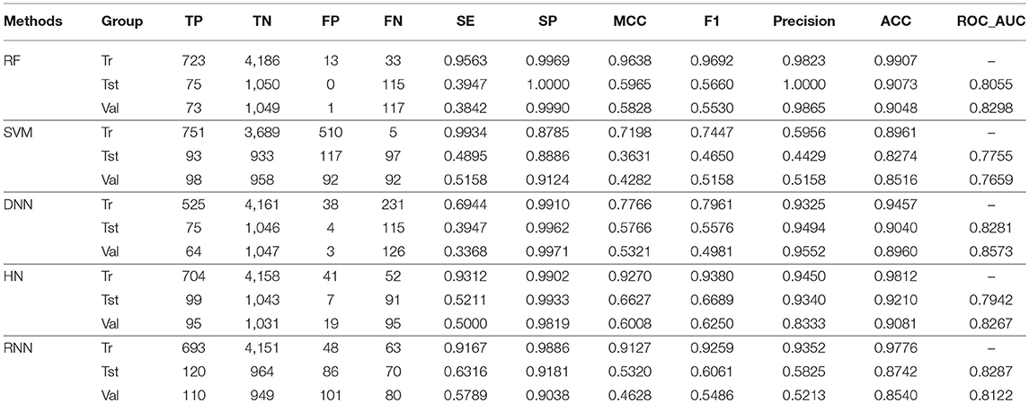
Table 3. The performance of constructed models based on the general molecular descriptors.
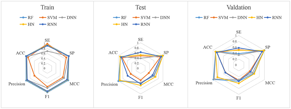
Figure 3. Radar plot of the descriptors-based classification models.
For the training set, all models gave very good SE, SP, MCC, F1-score, Precision, and ACC values. It should be noted that the SVM model showed lowest precision while DNN model exhibited lowest SE level. For the test and validation set, the indexes of all models exhibited a similar tendency, which tends to predict the compounds as inactivation due to the imbalanced distribution of active and inactive compounds. Among these models, the RNN model gave the highest SE value, while other indicators were not so well. It is worth noting that all indexes of the HN model were better than other models. In addition, the ROC-AUC is critical index for models performance and the ROC of all models are shown in Figure 4. For the test set, the RNN exhibited highest ROC-AUC (0.829), while for the validation set, DNN gave the highest ROC-AUC value of 0.857. Compared with the previous models, our models displayed a higher ROC value and ACC values.
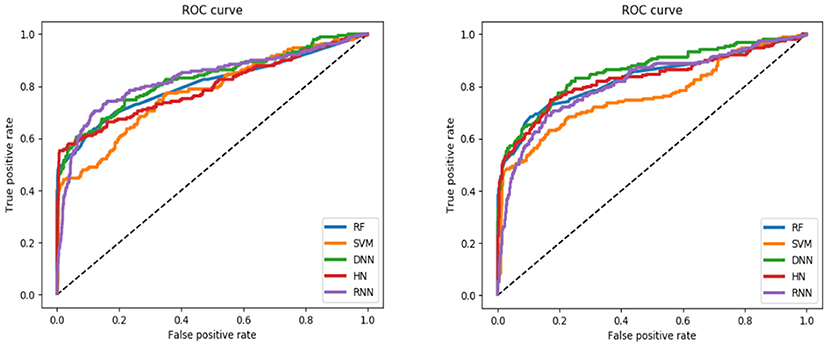
Figure 4. ROC curve of descriptors-based model (the left one is test set, the right one is validation set).
In general, the DNN model performed well for the external validation set predictions from the ROC-AUC metric, while the HN exhibited the higher ACC (0.908) than DNN as well as the MCC and F1 with 0.601 and 0.625, respectively. The RF model gave higher SP (0.999) and Precision (0.986). On the contrary, the RNN method gave higher SE value (0.579) than other models.
We further analyzed what kinds of molecular properties will affect the ARE toxicity of compounds. The Gini index was applied to sort the importance of molecular descriptors. The top 20 descriptors and their corresponding meanings are shown in Table 4. From the information of selected descriptors, it is clearly that the walk and path count descriptors hold a great impact on the ARE toxicity of compound. The 3D matrix-based descriptors, the edge adjacency indices as well as the atom-type E-state indices are also significant for the ARE toxicity of compound. Besides, the 2D matrix-based descriptors and 2D autocorrelations P_VSA-like descriptors also have a close correlation with ARE toxicity of compound.
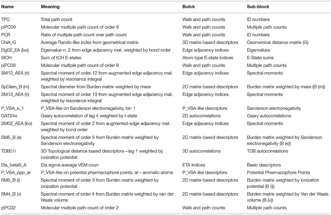
Table 4. 20 molecular descriptors selected by the RF method and Gini index analysis.
Performance Evaluation of Fingerprints-Based Classification Models
In addition to the general molecular descriptors, the molecular fingerprint is another effective method to represent the structural features of molecules. A typical frequency of fingerprints occurred in the 1,024 bins of the compounds in the data set is shown in Figure 5. The fingerprints features were applied to build the six models including DNN, HN, RNN, CNN, RF, and SVM. The results are presented in Table 5 and the radar plots are presented in Figure 6.
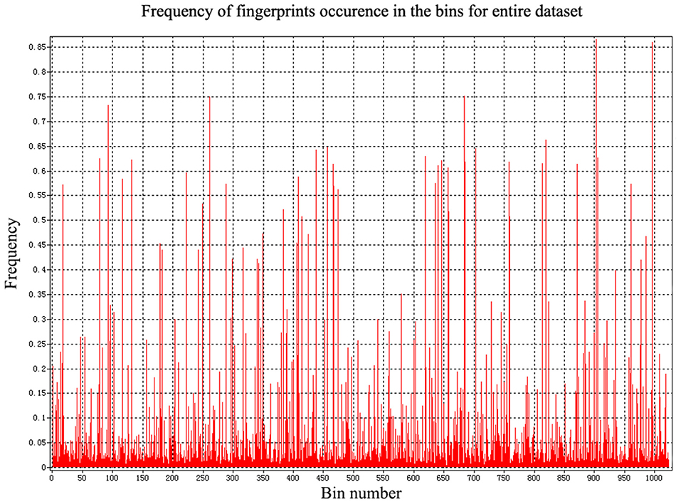
Figure 5. The frequency of fingerprints occurred in compounds.
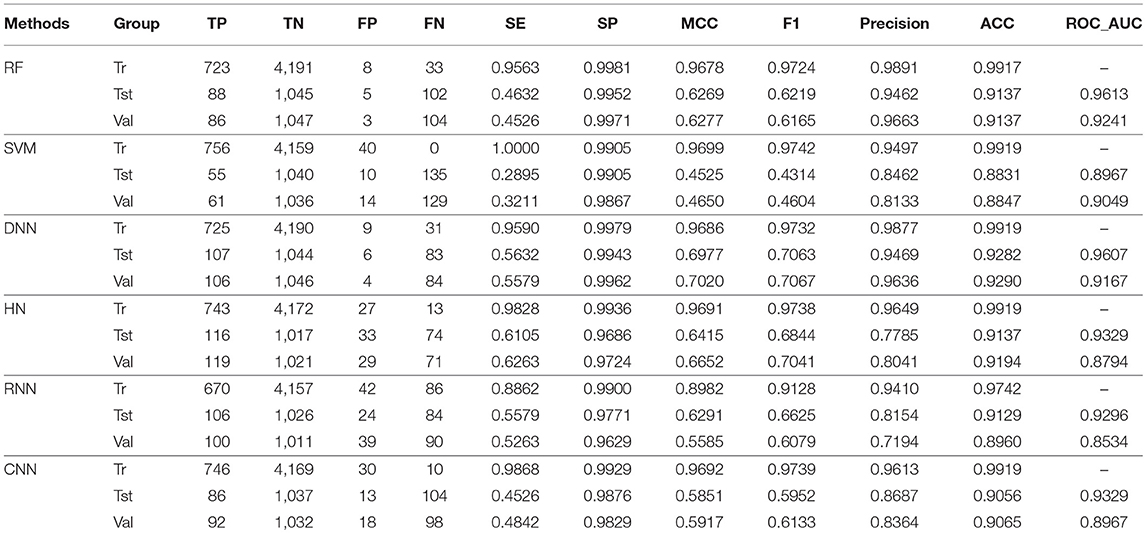
Table 5. The performance of constructed models based on the fingerprints.
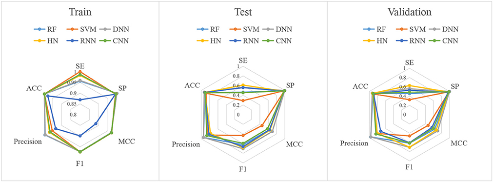
Figure 6. Radar plot of the fingerprints-based classification model.
For the training set, 5 out of all 6 models performed very well, except for the RNN method. According to the prediction results for test set, the value of SP, ACC, and precision were relatively stable, while the SE, F1-score and MCC showed different performance. The HN model exhibited the highest SE value while the SVM gave the lowest one. For the validation set, HN also performed better than other models on SE. As shown in Figure 7, all 6 models presented good ROC and large ROC-AUC, which were better than descriptor-based models. RF model has the highest ROC-AUC with 0.924 better than the DNN model with 0.917. However, the ACC of RF was lower than DNN model. But for the external validation set, Deep Learning methods had better generalization ability. Overall, the fingerprints-based models can give better prediction results than those based on molecular descriptors. The fingerprints of compounds were more useful than the descriptors for ARE toxicity prediction of compounds.
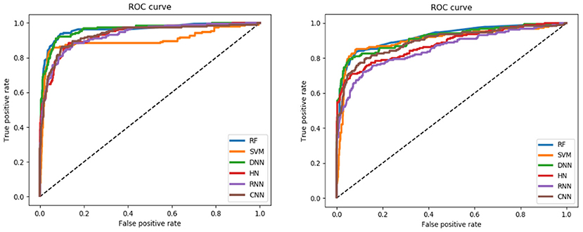
Figure 7. ROC curve of fingerprints-based model (left: test set, right: validation set).
Compared with the traditional machine learning methods, deep learning methods had better learning ability and they could extract the inherent characteristics of the data. For the models based on the molecular descriptors, DNN showed highest ROC_AUC and ACC, while the HN exhibited the best SE performance. Considering the fingerprints features, the performance of DNN model was still well and HN showed higher SE than other models.
The Comparisons Between Our Models and Other Models
We also compared the performance of our models with other reported models5. For the ARE toxicity prediction of Tox21 challenge data, the deep neural network models developed by Mayr et al. (2016) gave the best prediction results compared with other models. The best results they obtained had ROC-AUC 0.840, Balanced Accuracy 0.677 for the validation set. Other models displayed ROC-AUC ranging from 0.768 to 0.832 with the balanced accuracy between 0.519 and 0.729 using traditional machine learning methods, such as RF, SVM, and Naive Bayesian (shown in Table 6). Compared to their models and other models, our prediction models can give better prediction results. For the validation set, our best DNN model had ROC-AUC 0.917 and Accuracy 0.929.
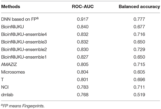
Table 6. The reported top 10 prediction models of ARE toxicity prediction in Tox 21 challenge data set.
Conclusions
In this study, multiple deep learning algorithms were used to predict the ARE toxicity of compounds based on two kinds of molecular features including the general molecular descriptors and fingerprints. The DNN model based on fingerprints had an outstanding performance with ROC-AUC 0.917 and ACC 0.929, while the DNN model based on the general molecular descriptors had relative lower predictive ability with ROC-AUC 0.857 and ACC 0.896, suggesting that the fingerprints can represent the structural features of compounds related to their ARE toxicity more comprehensively. Compared with the traditional machine learning model, the deep learning models had much better predictive ability. Our constructed accurate predictive models on ARE toxicity will be valuable to the assessment of toxicity of compounds.
Author Contributions
HL and CX conceived and designed the study. FB, DH, YL, and XY performed the experiment, analyzed the data, and wrote the manuscript.
Funding
This work was supported by the National Natural Science Foundation of China (Grant No. 21775060).
Conflict of Interest Statement
The authors declare that the research was conducted in the absence of any commercial or financial relationships that could be construed as a potential conflict of interest.
Supplementary Material
The Supplementary Material for this article can be found online at: https://www.frontiersin.org/articles/10.3389/fchem.2019.00385/full#supplementary-material
The ID of compounds used in our model is available in the Supplementary Material.
Footnotes
1. ^https://tripod.nih.gov/tox21/challenge/data.jsp
2. ^https://pubchem.ncbi.nlm.nih.gov/
3. ^https://en.wikipedia.org/wiki/Gini_coefficient
4. ^https://en.wikipedia.org/wiki/Principal_component_analysis
References
Abdelaziz, A., Spahn-Langguth, H., Karl-Werner, S., and Tetko, I. V. (2016). Consensus modeling for HTS assays using in silico descriptors calculates the best balanced accuracy in Tox21 challenge. Front. Environ. Sci. 4, 1–12. doi: 10.3389/fenvs.2016.00002
Bengio, Y., Simard, P., and Frasconi, P. (2002). Learning long-term dependencies with gradient descent is difficult. IEEE Trans. Neural Netw. 5, 157–166. doi: 10.1109/72.279181
Blomme, E. A., and Will, Y. (2016). Toxicology strategies for drug discovery: present and future. Chem. Res. Toxicol. 29, 473–504. doi: 10.1021/acs.chemrestox.5b00407
Dahl, G. E., Jaitly, N., and Salakhutdinov, R. (2014). Multi-task neural networks for QSAR predictions. arXiv: 1406.1231. Available online at: https://arxiv.org/pdf/1406.1231.pdf
Dang, N. L., Hughes, T. B., Miller, G. P., and Swamidass, S. J. (2018). Computationally assessing the bioactivation of drugs by N-dealkylation. Chem. Res. Toxicol. 31, 68–80. doi: 10.1021/acs.chemrestox.7b00191
Drwal, M. N., Siramshetty, V. B., Banerjee, P., Goede, A., Preissner, R., and Dunkel, M. (2015). Molecular similarity-based predictions of the Tox21 screening outcome. Front. Environ. Sci. 3:54. doi: 10.3389/fenvs.2015.00054
Fang, J., Yang, R., Gao, L., Zhou, D., Yang, S., Liu, A. L., et al. (2013). “Predictions of BuchE inhibitors using support vector machine (SVM) and naive Bayesian classification techniques,” in The 12th Meeting of The Asia Pacific Federation of Pharmacologists (Beijing), 3009–3020. doi: 10.1021/ci400331p
Filip, S. (2015). Prediction of compounds activity in nuclear receptor signaling and stress pathway assays using machine learning algorithms and low-dimensional molecular descriptors. Front. Environ. Sci. 3:77. doi: 10.3389/fenvs.2015.00077
Foloppe, N., and Chen, I. J. (2009). Conformational sampling and energetics of drug-like molecules. Curr. Med. Chem. 16, 3381–3413. doi: 10.2174/092986709789057680
Fraser, K., Bruckner, D. M., and Dordick, J. S. (2018). Advancing predictive hepatotoxicity at the intersection of experimental, in silico, and artificial intelligence technologies. Chem. Res. Toxicol. 31, 412–430. doi: 10.1021/acs.chemrestox.8b00054
Gawehn, E., Hiss, J. A., and Schneider, G. (2016). Deep learning in drug discovery. Mol. Inform. 35, 3–14. doi: 10.1002/minf.201501008
Gergo, B. (2016). Identifying biological pathway interrupting toxins using multi-tree ensembles. Front. Environ. Sci. 4:52. doi: 10.3389/fenvs.2016.00052
Glorot, X., and Bengio, Y. (2010). “Understanding the difficulty of training deep feedforward neural networks,” in Proceedings of the 13 th International Conference on Artificial Intelligence and Statistics (AISTATS) (Sardinia), 249–256. Available online at: http://proceedings.mlr.press/v9/glorot10a/glorot10a.pdf?hc_location=ufi
Graves, A., Mohamed, A.-R., and Hinton, G. (2013). “Speech recognition with deep recurrent neural networks,” in IEEE International Conference on Acoustics, Speech and Signal Processing (Toronto, ON: IEEE).
Gulshan, V., Peng, L., Coram, M., Stumpe, M. C., Wu, D., Narayanaswamy, A., et al. (2016). Development and validation of a deep learning algorithm for detection of diabetic retinopathy in retinal fundus photographs. JAMA 316, 2402–2410. doi: 10.1001/jama.2016.17216
Hanson, J., Yang, Y., Paliwal, K., and Zhou, Y. (2017). Improving protein disorder prediction by deep bidirectional long short-term memory recurrent neural networks. Bioinformatics 33, 685–692. doi: 10.1093/bioinformatics/btw678
Hayes, J. D., and Dinkova-Kostova, A. T. (2014). The Nrf2 regulatory network provides an interface between redox and intermediary metabolism. Trends Biochem. Sci. 39, 199–218. doi: 10.1016/j.tibs.2014.02.002
He, K., Zhang, X., Ren, S. G., and Sun, J. (2015). “Deep residual learning for image recognition,” in IEEE Conference on Computer Vision and Pattern Recognition (Boston, MA), 770–778. doi: 10.1109/CVPR.2016.90
Hinton, G. E., Srivastava, N., Krizhevsky, A., Sutskever, I., and Salakhutdinov, R. R. (2012). Improving neural networks by preventing co-adaptation of feature detectors. Comput. Sci. 3, 212–223. Available online at: https://arxiv.org/pdf/1207.0580.pdf
Hochreiter, S. (1991). Untersuchungen zu Dynamischen Neuronalen Netzen. [Master's Thesis], Institut Fur Informatik, Technische Universitat, Munchen.
Hochreiter, S., and Schmidhuber, J. (1997). Long short-term memory. Neural Comput. 9, 1735–1780. doi: 10.1162/neco.1997.9.8.1735
Hou, T.-Y., Weng, C.-F., and Leong, M. K. (2018). Insight analysis of promiscuous estrogen receptor α-ligand binding by a novel machine learning scheme. Chem. Res. Toxicol. 31, 799–813. doi: 10.1021/acs.chemrestox.8b00130
Huang, R., Xia, M., Nguyen, D.-T., Zhao, T., Sakamuru, S., Zhao, J., et al. (2016). Tox21 challenge to build predictive models of nuclear receptor and stress response pathways as mediated by exposure to environmental chemicals and drugs. Front. Environ. Sci. 3:85. doi: 10.3389/fenvs.2015.00085
Hughes, T. B., and Swamidass, S. J. (2017). Deep learning to predict the formation of quinone species in drug metabolism. Chem. Res. Toxicol. 30, 642–656. doi: 10.1021/acs.chemrestox.6b00385
Kaminski, G. A., Friesner, R. A., Tirado-Rives, J., and Jorgensen, W. L. (2001). Evaluation and reparametrization of the OPLS-AA force field for proteins via comparison with accurate quantum chemical calculations on peptides. J. Phys. Chem. B 105, 6474–6487. doi: 10.1021/jp003919d
Kennard, R. W., and Stone, L. A. (1969). Computer aided design of experiments. Technometrics 11, 137–148. doi: 10.1080/00401706.1969.10490666
Kode srl. (2017). Dragon (Software for Molecular Descriptor Calculation) Version 7.0.8. Available online at: https://chm.kode-solutions.net
Krizhevsky, A., Sutskever, I., and Hinton, G. E. (2012). “ImageNet classification with deep convolutional neural networks,” in Advances in Neural Information Processing Systems 25(NIPS2012), eds F. Pereira, C. Burges, L. Bottou, and K. Weinberger (Lake Tahoe), 1097–1105. Available online at: http://papers.nips.cc/paper/4824-imagenet-classification-with-deep-convolutional-neural-networks.pdf
Lecun, Y., Bengio, Y., and Hinton, G. (2015). Deep learning. Nature 521:436. doi: 10.1038/nature14539
Mamoshina, P., Vieira, A., Putin, E., and Zhavoronkov, A. (2016). Applications of deep learning in biomedicine. Mol. Pharm. 13, 1445–1454. doi: 10.1021/acs.molpharmaceut.5b00982
Mavroforakis, M. E., and Theodoridis, S. (2006). A geometric approach to Support Vector Machine (SVM) classification. IEEE Trans. Neural Netw. 17, 671–682. doi: 10.1109/TNN.2006.873281
Mayr, A., Klambauer, G., Unterthiner, T., and Hochreiter, S. (2016). DeepTox: toxicity prediction using deep learning. Front. Environ. Sci. 3:80. doi: 10.3389/fenvs.2015.00080
Ney, P. A., Sorrentino, B. P., Lowrey, C. H, and Nienhuis, A. W. (1990). Inducibility of the HS II enhancer depends on binding of an erythroid specific nuclear protein. Nucleic Acids Res. 18, 6011–6017. doi: 10.1093/nar/18.20.6011
Pedregosa, F., Varoquaux, G., Gramfort, A., Michel, V., and Thirion, B. (2011). Scikit-learn: machine learning in python. J. Mach. Learn. Res. 12, 2825–2830. doi: 10.1145/2786984.2786995
Raghunath, A., Sundarraj, K., Nagarajan, R., Arfuso, F., Bian, J., Kumar, A. P., et al. (2018). Antioxidant response elements: discovery, classes, regulation and potential applications. Redox Biol. 17, 297–314. doi: 10.1016/j.redox.2018.05.002
Rogers, D., and Hahn, M. (2010). Extended-connectivity fingerprints. J. Chem. Inf. Model. 50, 742–754. doi: 10.1021/ci100050t
Srivastava, R. K., Greff, K., and Schmidhuber, J. (2015). Highway Network. arXiv:1505.00387v2. Available online at: https://arxiv.org/pdf/1505.00387v2.pdf
Tieleman, T., and Hinton, G. (2012). Lecture 6.5-RMSProp, COURSERA: Neural Networks for Machine Learning. Technical Report.
Williams, R. J., and Zipser, D. (1989). A learning algorithm for continually running fully recurrent neural networks. Neural Comp. 1, 270–280. doi: 10.1162/neco.1989.1.2.27
Wu, K., and Wei, G. W. (2018). Quantitative toxicity prediction using topology based multitask deep neural networks. J. Chem. Inf. Model. 58, 520–531. doi: 10.1021/acs.jcim.7b00558
Xu, Y., Dai, Z., Chen, F., Gao, S., Pei, J., and Lai, L. (2015). Deep learning for drug-induced liver injury. J. Chem. Inf. Model. 55, 2085–2093. doi: 10.1021/acs.jcim.5b00238
Xu, Y., Pei, J., and Lai, L. (2017). Deep learning based regression and multiclass models for acute oral toxicity prediction with automatic chemical feature extraction. J. Chem. Inf. Model. 57, 2672–2685. doi: 10.1021/acs.jcim.7b00244
Yoshihiro, U. (2016). Rigorous selection of random forest models for identifying compounds that activate toxicity-related pathways. Front. Environ. Sci. 4:9. doi: 10.3389/fenvs.2016.00009
Keywords: antioxidant response elements (AREs), deep learning, toxicity, prediction, machine learning
Citation: Bai F, Hong D, Lu Y, Liu H, Xu C and Yao X (2019) Prediction of the Antioxidant Response Elements' Response of Compound by Deep Learning. Front. Chem. 7:385. doi: 10.3389/fchem.2019.00385
Received: 14 December 2018; Accepted: 14 May 2019;
Published: 31 May 2019.
Edited by:
José S. Torrecilla, Complutense University of Madrid, SpainReviewed by:
Yun Tang, East China University of Science and Technology, ChinaPeifeng Su, Xiamen University, China
Copyright © 2019 Bai, Hong, Lu, Liu, Xu and Yao. This is an open-access article distributed under the terms of the Creative Commons Attribution License (CC BY). The use, distribution or reproduction in other forums is permitted, provided the original author(s) and the copyright owner(s) are credited and that the original publication in this journal is cited, in accordance with accepted academic practice. No use, distribution or reproduction is permitted which does not comply with these terms.
*Correspondence: Huanxiang Liu, aHhsaXVAbHp1LmVkdS5jbg==; Cunlu Xu, Y2x4dUBsenUuZWR1LmNu
†These authors have contributed equally to this work