Abstract
A novel neural network adaptive filter algorithm is proposed to address the challenge of weak spectral signals and low accuracy in micro-spectrometer detection. This algorithm bases on error backpropagation (BP) and least mean square (LMS), introduces an innovative BP neural network model incorporating instantaneous error function and error factor to optimize the learning process. It establishes a network relationship through the input signal, output signal, error and step factor of the adaptive filter, and defines a training optimization learning method for this relationship. To validate the effectiveness of the algorithm, experiments were conducted on simulated noisy signals and actual spectral signals. Results show that the algorithm effectively denoises signals, reduces noise interference, and enhances signal quality, the SNR of the proposed algorithm is 3–4 dB higher than that of the traditional algorithm. The experimental spectral results showed that the proposed neural network adaptive filter algorithm combined with partial least squares regression is suitable for simultaneous detection of copper and cobalt based on ultraviolet-visible spectroscopy, and has broad application prospects.
1 Introduction
In the hydrometallurgy of extracting zinc, the current primary method of detecting the concentration information of copper and cobalt impurity metal ions relies on manual offline analysis (Zabiszak et al., 2021; Zhou et al., 2020; Sikder et al., 2018; Deluca et al., 2023). This approach means that the setting of industrial parameters in the process of hydrometallurgy lacks scientific basis. The real-time responsiveness is poor, the detection steps are cumbersome, and there is a significant lag time (Fawzy et al., 2023). The micro-fiber spectrometer, due to its characteristics such as miniaturization, integration, and rapid detection speed, is suitable for the online detection of multi-component substances in industrial settings (Attia et al., 2018; Giriraj and Sivakkumar, 2017; Martins et al., 2017; Dehghannasiri et al., 2017). However, as the micro-spectrometer adopts a single-beam structure and a CCD detector, when detecting the concentration of multiple metal ions in high zinc solution, issues arise due to the fluctuation of the light source, instrument circuit noise and interference from the base zinc ions (Jin et al., 2024; Zhang D. Y. et al., 2021; Liu et al., 2017; Zou et al., 2018). These factors lead to weak spectral signals and poor accuracy, severely affecting the precision of spectral detection.
In actual detection, noise is ubiquitous, encompassing high-frequency noise, low-frequency noise, white noise, and various other types of noise signals. To mitigate the impact of these noise signals, they need to be removed (Zhou et al., 2019; Ford et al., 2018; Huang and Chen, 2021; Li and Zhao, 2023). Signal enhancement algorithms are mainly aimed at processing signals where the signal-to-noise ratio is low due to strong noise interference (Lee et al., 2015). How to reduce noise in signals has always been a focal research topic in signal processing. Presently, commonly used signal enhancement algorithms both domestically and internationally include wavelet signal enhancement algorithms, Savitzky-Golay denoising enhancement algorithms, and LMS algorithms (Chu et al., 2021; Huang et al., 2020). The LMS algorithm, due to its low computational complexity, rapid convergence and high stability, has been widely applied worldwide. However, through research on the LMS algorithm, it is found that it inherently has some flaws. For instance, the conventional LMS algorithm has a relatively slow convergence speed and requires a longer denoising time (Sibtain et al., 2022). Therefore, it is necessary to improve the convergence speed and make the algorithm stable in a shorter time. It is clear that while traditional methods provide accuracy, they lack real-time capability and efficiency. Advanced spectroscopic techniques offer speed and integration but are hindered by noise and interference issues. Existing signal enhancement algorithms each have their strengths and weaknesses, with the LMS algorithm being notable for its balance of simplicity and performance despite its slower convergence.
In this paper, a neural network adaptive filtering algorithm (NNAF) based on BP (backpropagation) and LMS (Least Mean Square) is studied to improve the accuracy and real-time performance of online detection of impurity metal ion concentration (Zhang and So, 2020; Liu et al., 2015; Zhang and Luo, 2023; Zheng et al., 2020; Shi et al., 2021). As a widely used learning mechanism in neural network, BP algorithm adjusts the weight by calculating the output error and propagating it back to the network (Mancini et al., 2021). LMS algorithm is an adaptive filtering algorithm based on gradient descent principle, which has good convergence and robustness. The proposed neural network adaptive filtering algorithm integrates adaptive filtering and neural network error compensation (LeCun et al., 2015; Zhang C. et al., 2021; Huang et al., 2023). It adopts a new BP neural network model, combining instantaneous error function and error factor to improve the learning process. The network relationship is established through the input signal, output signal, error and step factor of the adaptive filter, and the training optimization method suitable for this relationship is determined. The experimental results show that the neural network adaptive filtering algorithm (NNAF) shows superior denoising ability, effectively reduces noise interference and improves signal quality.
2 NNAF adaptive denoising algorithm
2.1 NNAF algorithm
The LMS algorithm is an adaptive filtering method, extensively employed in the realm of signal processing and noise reduction. Despite its broad application, its convergence rate remains relatively slow. The schematic of the LMS principle is depicted in Figure 1. The backpropagation (BP) algorithm is an optimization method used within neural networks. It operates by calculating output errors and backpropagating them through the network for weight adjustment. The structure of the BP is illustrated in Figure 2. The BP algorithm boasts significant competence in addressing non-linear and intricate issues. However, during the early phases of training, weight adjustments might render the network’s output exceedingly sensitive. Noise at the inception can propagate throughout the entire network, resulting in unstable training outcomes. Therefore, by amalgamating the BP and LMS algorithms, a neural network adaptive filter method (NNAF) is proposed.
FIGURE 1

Schematic diagram of the LMS algorithm.
FIGURE 2

Diagram of the BP structure.
The NNAF algorithm leverages the noise reduction benefits of the LMS algorithm and the BP algorithm’s strength in optimizing complex non-linear problems, incorporating a new BP neural network model. During the backpropagation process, instantaneous error functions and error factors are introduced to optimize the learning procedure. The network relationship is established using the adaptive filter’s input signal, output signal, error, and step factor, and an optimized training procedure tailored to this relationship is identified. This algorithm successfully combines adaptive filtering with neural network error compensation. Through this approach, the NNAF algorithm effectively minimizes noise interference and enhances signal quality.
2.2 Implementation of the NNAF algorithm
The implementation of the NNAF adaptive denoising algorithm is primarily an efficient and intertwined process. This procedure integrates the strategies of LMS filtering and BP optimization, fully harnessing the strengths of both to enhance denoising performance. The schematic of this algorithm is depicted in Figure 3.
FIGURE 3

Schematic diagram of the NNAF algorithm.
Where and are the input signals for the BP neural network, and is the output of the neural network training results. The NNAF algorithm establishes a learning network structure, seeking the optimal learning step factor through the error and input signal . By learning from given sample data, it establishes a real-time data correlation model. The rules for updating the parameters of the NNAF algorithm are Equation 1, Equation 2 and Equation 3.
To ensure the convergence of the neural network algorithm, must satisfy (where is the maximum eigenvalue and is positive). Using ensures that is still influenced by the changes in the output signal and error. In practical applications, and can be determined experimentally. To speed up convergence, instantaneous error function and error factor proposed by this algorithm are shown in Equation 4 and Equation 5.
In Equation 4, the steepness of the Sigmoid function is directly determined by parameter , which is inversely related to the speed at which the function curve rises. characterizes the range of values of the dependent variable in the Sigmoid function, determining the height of the curve.
In Equation 5, represents the error factor, and represents the rate of exponential growth. It can also be understood as the rate at which the correction factor is adjusted. The larger is, the greater the instantaneous error, and the greater the correction to the step factor. At this time, the step factor at the initial moment is larger, which further updates the required weight vector value. Through experimental simulation, the optimal value of parameter is 5, and the optimal value of parameter is 6., as shown in Equation 6:
The NNAF algorithm optimizes the learning process by incorporating an instantaneous error function and error factor . It uses the input signal , output signal , error , and step factor of the adaptive filter to establish a network relationship and determines the training optimization learning steps for this relationship. The flowchart of the NNAF algorithm is shown in Figure 4. First, initialize the step vector and process the input signal with LMS filtering. Then, the error between the target output and the filter output is backpropagated to BP. By calculating the gradient of the error and then updating the step factor in the negative direction of the gradient, the output of the filter becomes closer to the expected output. This also further reduces the error, achieving global optimization. Finally, the LMS algorithm and BP algorithm interactively feedback. When the error signal is less than , the iteration ends, and the filtered signal is output.
FIGURE 4

Flowchart of the NNAF algorithm.
3 Experimental
3.1 Simulated data
The simulation data is used to select the adaptive step factor of the neural network adaptive filter algorithm (NNAF) and verify the denoising performance. The pure signal uses sine wave signal provided by MATLAB software, and then adds noise with signal-to-noise ratio (SNR) of 15 dB. The original signal and noisy signal are shown in Figure 5.
FIGURE 5
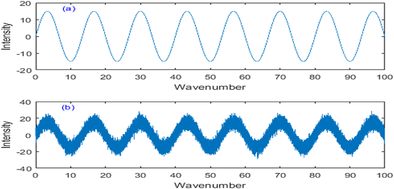
Simulated original signal and noisy signal. (A) Original signal. (B) Noisy signal.
3.2 Experimental spectral signal
Add the standard solution of copper, cobalt and zinc, 7.5 ml of acetic acid-sodium acetate solution and 5.00 ml of nitroso R salt solution in turn into a 25 ml calibration flask and dilute with distilled water. Shake well to complete the reaction of the elements to be detected, and prepare a blank reagent reference in the same way. The solution to be tested and the reference solution were placed in a 1 cm cuvette and measured by the Optosky ATP2000 spectrophotometer in the wavelength range of 200–1,100 nm. The final concentration ranges were 0.5–5 mg/L for copper, and 0.3–3 mg/L for cobalt. All measured spectra were the average of 5 replicates.
4 Results and discussion
4.1 Comparison of convergence performance
In order to verify the effectiveness of NNAF algorithm, the performance of NNAF algorithm is compared with other commonly used algorithms. The comparison of the convergence error performance of the three algorithms is shown in
Figure 5. The input signal is a noisy sine wave, and the simulation parameters are set as follows.
1) The order of the filter is set 10. The initial weight of the adaptive filter is defined as 0, and added noise is a zero-mean independent Gaussian random sequence with a variance of 0.04.
2) For the fixed-step LMS algorithm, its learning step factor is a small positive number, step factor set to 0.008. For the variable step-size algorithm, its step size is variable. and are 0.009, 0.0006 in the algorithm respectively.
3) Average statistical time is 20, and the sample size is 1,000. The greed algorithm is used in the NNAF model to find training samples, with some data shown in Table 1.
4) A BP model is established, which includes an input vector with 10 components (assuming the input signal of the adaptive filter is 12 and the deviation is 2) and 25 hidden units. The model is trained through the neural network to scan the output results, thereby generating the optimal step size factor .
TABLE 1
| Input signal x(n) | Error | u |
|---|---|---|
| −1.1676 1.0718 1.1786 1.5808 -1.3713 -0.9793 -0.7802 1.7091 -0.0351 0.1680 | 0.3008 | 0.310 |
| 0.7880 0.7925 0.1972 -0.0696 -0.0867 -0.0277 -0.0048 0.0084 0.0157 -0.0065 | 0.6324 | 0.800 |
| 0.8307 0.8292 0.2088 -0.0964 -0.1078 -0.0334 0.0147 0.0242 0.0162 0.0068 | −0.4133 | 0.5090 |
| 0.0070 0.0141 0.0212 0.0282 0.0352 0.0424 0.0494 0.0565 0.0636 0.0706 | −0.2865 | 0.0037 |
| 0.7560 0.7489 0.7418 0.7348 0.6995 0.6924 0.6854 -1.9866-1.9364 -1.9601 | 0.0183 | 0.4396 |
Partial training sample data of the BP model.
It can be observed from Figure 6 that the NNAF algorithm allows the adaptive filter to achieve higher convergence speed compared with the other three algorithms.
FIGURE 6

Error convergence curve diagram.
4.2 Noise elimination of simulation data
The denoising effect of NNAF method was compared with that of other denoising methods. The comparison of denoising effects using different methods is shown in Figure 7. In Figure 7A, the denoised signal using fixed step LMS method retained a lot of noise, and the denoising effect was obviously poor. In Figure 7B, the denoised signal using variable step LMS method was relatively smooth, but the denoising effect at the beginning is not good. In Figure 7C, the denoised signal using the proposed NNAF method is smooth and retains the peak characteristics, which is in good agreement with the original signal, so it has good denoising performance.
FIGURE 7

Comparison of denoising effects using different methods. (A) Fixed step LMS algorithm. (B) Variable step LMS algorithm. (C) NNAF algorithm.
In order to further verify the performance of the proposed NNAF method, different signal-to-noise ratios are added to the original signal. The signal-to-noise ratio (SNR) and root mean square error (RMSE) of denoised signals obtained by different methods are shown in Table 2. Compared with other methods, the denoised signal using NNAF method has the highest SNR and the smallest RMSE under different signal-to-noise ratios. Therefore, the simulation results strongly show that the proposed NNAF algorithm achieves superior denoising performance, which verifies its theoretical feasibility.
TABLE 2
| Denoising methods | 5 dB | 15 dB | 25 dB | |||
|---|---|---|---|---|---|---|
| SNR/dB | RMSE | SNR/dB | RMSE | SNR/dB | RMSE | |
| Fixed step LMS algorithm | 7.1391 | 0.5493 | 22.4684 | 0.5391 | 29.2929 | 0.3634 |
| Variable step LMS algorithm | 9.7945 | 0.3545 | 27.5210 | 0.2987 | 32.4876 | 0.2514 |
| NNAF algorithm | 16.7149 | 0.2945 | 28.2662 | 0.2514 | 36.3937 | 0.1603 |
The calculation results of the denoised signal by different methods.
4.3 Spectral processing
The proposed NNAF method was applied to the experimental ultraviolet-visible spectral signal. Figure 8A shows absorption spectra of copper (Cu) in the wavelength range of 200–1,100 nm, where the concentration of copper ranged from 0.5 to 6.0 mg/L. Figure 8B shows absorption spectra of cobalt (Co), where the concentration of cobalt ranged from 0.3 to 3.0 mg/L. As can be seen from Figure 8, the spectral signals of copper and cobalt are seriously disturbed by noise. The maximum absorbance of copper and cobalt are at the wavelengths of 484.66 nm and 503.47 nm, respectively. In order to evaluate the linearity, the calibration curves of copper and cobalt at the maximum absorbance were constructed. As can be seen from Figures 8C, D, the linearity of copper and cobalt is poor. The linear equation and linear coefficient of copper is: Abs = 0.1359 CCu+ 0.0061 (R2 = 0.9908). The linear equation and linear coefficient of cobalt is Abs = 0.1834 CCo+ 0.5801 (R2 = 0.9926). Therefore, it is necessary to denoise the experimental spectrum and improve the detection accuracy.
FIGURE 8

Acquisition of spectral signal. (A) Absorbance spectra of Cu. (B) Absorbance spectra of Co. (C) Calibration curves of copper. (D) Calibration curves of cobalt.
The Optosky ATP2000 micro spectrometer has the advantages of intelligence, miniaturization, modularization and fast detection speed, but it adopts single beam structure and CCD detector, which leads to noise affecting the detection performance of spectrometer. Therefore, the spectral signal is disturbed by noise, the accuracy of simultaneous detection of copper and cobalt will be seriously affected if the spectral data is directly modeled without denoising pretreatment. The proposed NNAF method is used to process spectral signal and eliminate high-frequency and low-frequency noise. Figure 9A shows the denoising signal of copper. Figure 9B shows the denoising signal of cobalt. As can be seen from Figures 9A, B, the denoised signals of copper and cobalt are smooth, and the signal shape is consistent with the expectation. In order to evaluate the performance of NNAF method, Figures 9C, D show the calibration curves of the denoised copper and cobalt signals at the maximum absorbance. The correlation coefficients of Cu and Co are 0.9952 and 0.9967, respectively. The results show that the proposed NNAF method significantly improves the linear relationship between copper and cobalt, which is beneficial to improve the accuracy of simultaneous detection of copper and cobalt.
FIGURE 9

Spectral processed signal using NNAF method. (A) Absorbance spectra of Cu. (B) Absorbance spectra of Co. (C) Calibration curves of copper. (D) Calibration curves of cobalt.
4.4 Simultaneous detection of copper and cobalt
In order to evaluate the performance of NNAF algorithm in experimental spectrum processing, we prepared 10 groups of mixed solutions containing different proportions of copper and cobalt, in which the zinc concentration was fixed at 20 g/L for reference. PLS (partial least square method) and NNAF-PLS (neural network adaptive filter algorithm combined with partial least square method) were used to simultaneously detect copper and cobalt. The root mean square error of prediction values (RMSEP) and average relative deviation (ARD) are used as evaluation indexes, and the predicted concentrations of cop-per and cobalt are shown in Table 3. It can be concluded from Table 3 that the prediction performance of NNAF–PLS method is far superior to that of PLS method. Using NNAF–PLS method to detect copper and cobalt simultaneously, the RMSEP for copper and cobalt were 0.104 and 0.048, respectively; the ARD of copper and cobalt were 3.342% and 2.521%, respectively, which meets industrial production indicators.
TABLE 3
| No. | Actual value (mg/L) | Predicted value by PLS | Predicted value by NNAF–PLS | |||
|---|---|---|---|---|---|---|
| Cu | Co | Cu | Co | Cu | Co | |
| 1 | 2.0 | 1.5 | 1.902 | 1.563 | 1.963 | 1.519 |
| 2 | 3.0 | 1.2 | 3.284 | 1.302 | 2.884 | 1.241 |
| 3 | 5.0 | 2.7 | 5.425 | 2.535 | 5.106 | 2.668 |
| 4 | 4.0 | 0.6 | 4.361 | 0.641 | 4.145 | 0.612 |
| 5 | 1.5 | 3.0 | 1.417 | 3.212 | 1.436 | 3.109 |
| 6 | 3.5 | 0.3 | 3.287 | 0.322 | 3.397 | 0.311 |
| 7 | 4.5 | 0.9 | 4.922 | 0.944 | 4.703 | 0.931 |
| 8 | 1.0 | 2.4 | 0.934 | 2.142 | 0.962 | 2.345 |
| 9 | 2.5 | 2.1 | 2.773 | 2.251 | 2.556 | 2.145 |
| 10 | 0.5 | 1.8 | 0.531 | 1.907 | 0.521 | 1.839 |
| The average relative deviation (%) | 7.661 | 6.872 | 3.342 | 2.521 | ||
| RMSEP | 0.267 | 0.138 | 0.104 | 0.048 | ||
The predicted results of copper and cobalt by PLS and NNAF–PLS methods.
Figure 10 shows the calibration curve between the predicted value and the actual value of copper and cobalt. From Figure 10, it can be seen that the predicted values and the actual values of copper and cobalt are almost the same, and the correlation coefficient (R2) of copper is 0.9975 and that of cobalt is 0.9987. The experimental results show that this proposed NNAF method is suitable for on-line detection of copper and cobalt in zinc hydro-metallurgy, and has broad application prospects.
FIGURE 10

Predicted and actual values of copper and cobalt. (A) Copper. (B) Cobalt.
5 Conclusion
This paper presents a neural network adaptive filter algorithm (NNAF) based on error backpropagation (BP) and the least mean square (LMS). Through in-depth research and experimental processing of actual signals, we found that this algorithm can effectively reduce noise interference and improve signal quality, showing great potential for application. The algorithm fully leverages the advantages of both BP and LMS. It not only utilizes BP’s efficacy in error backpropagation but also incorporates the denoising characteristics of LMS, further enhancing the performance of the denoising algorithm. The experimental spectral results showed that the proposed neural network adaptive filter algorithm (NNAF) combined with partial least squares regression is suitable for simultaneous detection of copper and cobalt based on ultraviolet-visible spectroscopy. The work in this paper is an effective attempt to detect polymetallic ions online in the process of zinc hydrometallurgy, and the proposed neural network adaptive filter method is also suitable for other spectral signals, such as infrared spectra, Raman spectra, and more.
Statements
Data availability statement
The raw data supporting the conclusions of this article will be made available by the authors, without undue reservation.
Author contributions
BW: Data curation, Investigation, Project administration, Software, Visualization, Writing–original draft. FZ: Conceptualization, Funding acquisition, Investigation, Methodology, Project administration, Visualization, Writing–review and editing.
Funding
The author(s) declare that financial support was received for the research, authorship, and/or publication of this article. This work was supported in part by the National Natural Science Foundation of China under Grant 62273360, in part by Hunan Provincial Natural Science Foundation of China under Grant 2022JJ50238, in part by Research Foundation of Hunan Provincial Education Department under Grant 22B0745, in part by Research Innovation Project of Hunan Provincial Education Department under Grant CX20231295, and in part by Research Foundation of Shaoyang Science and Technology Bureau under Grant 2022GX4072.
Acknowledgments
Acknowledgment is due to the expert groups of Hongqiu Zhu, as well as to all contributors.
Conflict of interest
The authors declare that the research was conducted in the absence of any commercial or financial relationships that could be construed as a potential conflict of interest.
Publisher’s note
All claims expressed in this article are solely those of the authors and do not necessarily represent those of their affiliated organizations, or those of the publisher, the editors and the reviewers. Any product that may be evaluated in this article, or claim that may be made by its manufacturer, is not guaranteed or endorsed by the publisher.
References
1
Attia K. A. El-Abasawi N. M. El-Olemy A. Abdelazim A. H. (2018). Application of different spectrophotometric methods for simultaneous determination of elbasvir and grazoprevir in pharmaceutical preparation. Spectrochim. Acta A, Mol. Biomol. Spectrosc.189, 154–160. 10.1016/j.saa.2017.08.026
2
Chu Y. Chan S. C. Zhou Y. Wu M. (2021). A new diffusion variable spatial regularized LMS algorithm. Signal process.188, 108207. 10.1016/j.sigpro.2021.108207
3
Dehghannasiri R. Esfahani M. S. Dougherty E. R. (2017). Intrinsically Bayesian robust Kalman filter: an innovation process approach. IEEE Trans. Signal Process.65 (10), 2531–2546. 10.1109/tsp.2017.2656845
4
Deluca M. Hu H. L. Popov M. N. Spitaler J. Dieing H. (2023). Advantages and developments of Raman spectroscopy for electroceramics. Commun. Mater4, 78. 10.1038/s43246-023-00400-4
5
Fawzy M. G. Mostafa A. A. Shalaby A. Sayed R. A. (2023). Green-assisted spectrophotometric techniques utilizing mathematical and ratio spectra manipulations to resolve severely overlapped spectra of a cardiovascular pharmaceutical mixture. Spectrochim. Acta. A295, 122588. 10.1016/j.saa.2023.122588
6
Ford J. L. Green M. H. Green J. B. Oxley A. Lietz G. (2018). Intestinal β-carotene bioconversion in humans is determined by a new single-sample, plasma isotope ratio method and compared with traditional and modified area-under-the-curve methods. Arch. Biochem. Biophys.653, 121–126. 10.1016/j.abb.2018.06.015
7
Giriraj P. Sivakkumar T. (2017). Simultaneous estimation of dutasteride and tamsulosin hydrochloride in tablet dosage form by vierordt’s method. Arab. J. Chem.10, S1862–S1867. 10.1016/j.arabjc.2013.07.013
8
Huang W. Chen C. (2021). A novel quaternion kernel LMS algorithm with variable kernel width. IEEE Trans. Signal Process68, 2715–2719. 10.1109/tcsii.2021.3056452
9
Huang W. Chen C. Yao X. Li Q. (2020). Diffusion fused sparse LMS algorithm over networks. Signal process.171, 107497. 10.1016/j.sigpro.2020.107497
10
Huang W. Shan H. Xu J. Yao X. (2023). Adaptive diffusion pairwise fused Lasso LMS algorithm over networks. IEEE Trans. Neural Netw. Learn. Syst.34, 5816–5827. 10.1109/tnnls.2021.3131335
11
Jin X. K. He H. N. Ming L. Jiang J. J. Qi X. T. Zhu C. Y. (2024). Detection of moisture content of polyester fabric based on hyperspectral imaging and BP neural network. IEEE Signal Process. Mag.321, 124678. 10.1016/j.saa.2024.124678
12
LeCun Y. Bengio Y. Hinton G. (2015). Deep learning. Nature521, 436–444. 10.1038/nature14539
13
Lee H. S. Kim S. E. Lee J. W. Song W. J. (2015). A variable step-size diffusion LMS algorithm for distributed estimation. IEEE Trans. Signal Process.63, 1808–1820. 10.1109/tsp.2015.2401533
14
Li L. Zhao X. (2023). Variable step-size LMS algorithm based on hyperbolic tangent function. Circuits Syst. Signal Process.42, 4415–4431. 10.1007/s00034-023-02303-8
15
Liu J. Zhao H. Quan H. (2015). Iteration-based variable step-size LMS algorithm and its performance analysis. J. Electron. Inf. Technol.37, 1674–1680. 10.11999/JEIT141501
16
Liu P. Nie Y. Z. Xia Q. L. Guo G. h. (2017). Structural and electronic properties of arsenic nitrogen monolayer. Phys. Lett. A381, 1102–1106. 10.1016/j.physleta.2017.01.026
17
Mancini T. Calvo-Pardo H. Olmo J. (2021). Extremely randomized neural networks for constructing prediction intervals. Neural Netw.144, 113–128. 10.1016/j.neunet.2021.08.020
18
Martins A. Talhavini M. Vieira M. L. Zacca J. J. Braga J. W. B. (2017). Discrimination of whisky brands and counterfeit identification by UV-Vis spectroscopy and multivariate data analysis. Food Chem.229, 142–151. 10.1016/j.foodchem.2017.02.024
19
Shi L. Ding X. Li M. Liu Y. (2021). Research on the capability maturity evaluation of intelligent manufacturing based on firefly algorithm, sparrow search algorithm, and BP neural network. Complexity2021. 10.1155/2021/5554215
20
Sibtain D. Gulzar M. M. Shahid K. Javed I. Murawwat S. Hussain M. M. (2022). Stability analysis and design of variable step-size P&O algorithm based on fuzzy robust tracking of MPPT for standalone/grid connected power system. Sustainability14, 8986. 10.3390/su14158986
21
Sikder M. Lead J. R. Chandler G. Baalousha M. (2018). A rapid approach for measuring silver nanoparticle concentration and dissolution in seawater by UV-Vis. Sci. Total. Environ.618, 597–607. 10.1016/j.scitotenv.2017.04.055
22
Zabiszak M. Frymark J. Nowak M. Grajewski J. Stachowiak K. Kaczmarek M. T. et al (2021). Influence of d-electron divalent metal ions in complex formation with L-tartaric and L-malic acids. Molecules26, 5290. 10.3390/molecules26175290
23
Zhang C. Yu S. Li G. Xu Y. (2021b). The recognition method of MQAM signals based on BP neural network and bird swarm algorithm. IEEE Access9, 36078–36086. 10.1109/access.2021.3061585
24
Zhang D. Y. Satapathy S. C. Guttery D. C. Górriz J. M. Wang S. H. (2021a). Improved breast cancer classification through combining graph convolutional network and convolutional neural network. Inf. Process. and Manag.58, 102439. 10.1016/j.ipm.2020.102439
25
Zhang H. Luo D. L. (2023). Deep MCANC: a deep learning approach to multi-channel active noise control. Neural Netw.158, 318–327. 10.1016/j.neunet.2022.11.029
26
Zhang S. So H. C. (2020). Diffusion average-estimate bias-compensated LMS algorithms over adaptive networks using noisy measurements. IEEE Trans. Signal Process.68, 4643–4655. 10.1109/tsp.2020.3014801
27
Zheng G. Wang H. Li Y. (2020). Spectral signal denoising algorithm based on improved LMS. Spectrosc. Spect. Anal.40 (02), 643–649.
28
Zhou F. Li C. Yang C. Li Y. (2019). A spectrophotometric method for simultaneous determination of trace ions of copper, cobalt, and nickel in the zinc sulfate solution by ultraviolet-visible spectrometry. Spectrochim. Acta A223, 117370. 10.1016/j.saa.2019.117370
29
Zhou F. Li Y. Zhu H. Zhou C. Li C. (2020). Signal enhancement algorithm for on-line detection of multi-metal ions based on ultraviolet-visible spectroscopy. IEEE Access8, 16000–16008. 10.1109/access.2020.2967021
30
Zou Z. Deng Y. Hu J. Jiang X. Hou X. (2018). Recent trends in atomic fluorescence spectrometry towards miniaturized instrumentation—a review. Anal. Chim. Acta1019, 25–37. 10.1016/j.aca.2018.01.061
Summary
Keywords
neural network adaptive filter, signal processing, noise reduction, quantitative analysis, ultraviolet-visible spectroscopy
Citation
Wu B and Zhou F (2024) Application of neural network adaptive filter method to simultaneous detection of polymetallic ions based on ultraviolet-visible spectroscopy. Front. Chem. 12:1409527. doi: 10.3389/fchem.2024.1409527
Received
02 April 2024
Accepted
27 August 2024
Published
05 September 2024
Volume
12 - 2024
Edited by
Ricard Boqué, University of Rovira i Virgili, Spain
Reviewed by
Chunfen Jin, Honeywell UOP, United States
Mansoor Ahmed Khuhro, Sindh Madressatul Islam University, Pakistan
Pinial Khan, Sindh Agriculture University, Pakistan
Updates
Copyright
© 2024 Wu and Zhou.
This is an open-access article distributed under the terms of the Creative Commons Attribution License (CC BY). The use, distribution or reproduction in other forums is permitted, provided the original author(s) and the copyright owner(s) are credited and that the original publication in this journal is cited, in accordance with accepted academic practice. No use, distribution or reproduction is permitted which does not comply with these terms.
*Correspondence: Fengbo Zhou, fbzhou5018@126.com
Disclaimer
All claims expressed in this article are solely those of the authors and do not necessarily represent those of their affiliated organizations, or those of the publisher, the editors and the reviewers. Any product that may be evaluated in this article or claim that may be made by its manufacturer is not guaranteed or endorsed by the publisher.