Temperature field study of LSAM-50 flexible base asphalt pavement

Recent research has shown that increasing the aggregate particle size and forming a compact, skeleton-dense structure can effectively control reflective cracking and improve rutting resistance of the road, thereby extending the service life of the pavement. To this end, the group developed a super-large particle size LSAM-50 mix (with a maximum nominal particle size ≥50 mm), characterized by low engineering costs, excellent rutting resistance, and the potential to extend the service life of asphalt pavements. The temperature field of LSAM-50 pavement serves as the foundation for evaluating the temperature sensitivity of the material, accurately analyzing the mechanical response of the pavement, and designing a rational pavement structure. Under the combined effects of sunlight, rainfall, wind, and other environmental factors, the internal temperature of asphalt pavement undergoes continuous cyclic changes. During the heat conduction process into the pavement depth, part of the heat is absorbed by the pavement material, resulting in a temperature gradient within the pavement structure. Therefore, the interaction between the natural environment, pavement materials, and other factors is centrally reflected in the spatial and temporal distribution characteristics of the pavement temperature field. Although numerous studies on pavement temperature distribution and prediction models have been conducted both domestically and internationally, significant differences still exist in the temperature distribution of pavements with varying structures and materials, as well as in different regions and terrains.

1 Introduction

Asphalt mixtures exhibit strong temperature sensitivity: at low temperature, they behave as brittle hard solids; at room temperature, as viscoelastic materials; at high temperature, they are in the flow state. Therefore, the deterioration of the pavement performance is directly related to temperature changes. Numerous Chinese construction codes and standards define precise temperature control ranges for the construction process and provide technical guidelines for adapting construction practices to temperature variations. These provisions underscore the critical role of temperature in influencing the performance characteristics of asphalt pavements (MOT, 2004; MOT, 2011; MOT, 2017). In the summer, high temperatures cause the pavement structure to experience viscous flow of the mixture, leading to rutting. In the winter, temperature drops or repeated cycles of heating and cooling result in internal thermal stresses that exceed the material’s tensile strength causing temperature-induced shrinkage cracks (Li et al., 2015; Im et al., 2013; Fan et al., 2022). Kong et al. studied the effect of temperature on the compressive strength and modulus of elasticity of cemented asphalt mortar. The results showed that both the compressive strength and modulus of elasticity decrease with the increase in temperature, and that higher asphalt content increases the sensitivity of the mixture’s strength to the temperature changes (Kong et al., 2014). Pérez-Jiménez et al. investigated the coupling effect of temperature and load on the low-temperature cracking performance of asphalt mixtures, and the results showed that at −15°C, asphalt mixtures lose their viscosity and become more rigid (Pérez-Jiménez et al., 2013). Cheng et al. investigated the fatigue performance of asphalt pavements under the combined influence of temperature and stress, and the results showed that the fatigue life of asphalt mixtures decreases with increasing strain and increases with temperature (Cheng et al., 2021). Boussabnia et al. investigated the effect of temperature on the fatigue performance of high-modulus asphalt mixtures and found that their fatigue performance improved at low temperatures (Boussabnia et al., 2023). Jiang et al. conducted repetitive loading tests at different temperatures and various peripheral pressures, establishing load–temperature master curves for asphalt mixtures and evaluating the effect of temperature on their permanent deformation (Jiang et al., 2018), which highlights the large influence of temperature on the performance of asphalt pavements. Therefore, it is important to understand the distribution of internal temperature field of asphalt pavement under service conditions for accurately assessing its usage conditions and performance characteristics (Yang et al., 2010; Qian et al., 2021; Aliha et al., 2015). Since 1957, when American researchers first began studying the temperature field of asphalt pavement, the internal temperature field has become a key focus of international research (Barber, 1957). Subsequently, Germany, Britain, Japan, and many other countries have conducted research on the temperature distribution characteristics of asphalt and cement concrete pavements (Williamson, 1972; Kondo and Miura, 1976; Hermansson, 2001).

Currently, the main solution methods for predicting the asphalt pavement temperature field include theoretical analysis and statistical analysis, both of which are valuable for analyzing the temperature distribution characteristics of asphalt pavement (Adwan et al., 2021). In early studies, researchers primarily developed temperature field prediction models using statistical and theoretical analysis methods. The theoretical analysis method combines the thermodynamic properties of asphalt pavement and the location of the meteorological data, applying meteorological data and the basic theory of heat transfer to determine boundary conditions and establish a solution method for predicting the asphalt pavement temperature field. Qi et al. studied the variation patterns of the temperature field in open-graded friction course (OGFC) asphalt pavement and developed an analytical solution for the temperature field of OGFC pavement structures using mathematical and physical methods based on thermodynamic and heat transfer principles. The accuracy of the model is verified by comparing the outdoor test data obtained from large Marshall specimens with the analytical solution of the temperature field. The results showed that the field analysis model for OGFC asphalt pavement structures can predict temperature changes under different asphalt–rock ratios, as well as over time and at varying pavement depths (Qi et al., 2023). Hamed and Makki (2011), Crevier and Delage (2001), and Zhang et al. (2003) all used this method to develop asphalt pavement temperature prediction models. Statistical analysis involves performing a regression analysis on a large number of field measurements to derive a quantitative relationship between pavement temperature and environmental factors. In 1987, the United States’ Long-Term Pavement Performance (LTPP) project used regression analysis to develop a model for predicting asphalt pavement temperature based on a large amount of monitoring data such as atmospheric temperature, solar radiation, and their correlation with pavement temperature (Diefenderfer et al., 2006). Bosscher et al. (1998), Kršmanc et al. (2013), and Yin et al. (2019) also used this method.

Existing studies have predominantly focused on the thermal field characteristics of conventional dense-graded asphalt concrete, using methodologies based on single-point monitoring and steady-state heat transfer assumptions, which fail to adequately address the influence of material internal heterogeneity on heat transfer pathways. In contrast to homogeneous dense-graded materials, the skeletal porous structure of large-aggregate LSAM-50 flexible base layers forms unique heat exchange pathways, where discontinuous interfaces (e.g., aggregate-binder interfaces and pore networks) significantly reduce heat transfer efficiency, while air microcirculation induced by pore channels may alter the temperature gradient distribution patterns. These characteristics align closely with the findings of Stukhlyak et al., who demonstrated through multiscale analysis that discontinuous interfaces and multiphase coupling effects within materials can significantly alter energy transfer modes under external loading, with microscopic heterogeneity ultimately governing macroscopic behavior through mesoscopic dissipation mechanisms (Stukhlyak et al., 2015). Nevertheless, research on discontinuous heat transfer structures, such as LSAM-50, remains notably insufficient. To address this gap, this study investigates LSAM-50 using a multiscale analytical framework inspired by research on heterogeneous materials. In contrast to traditional single-point temperature monitoring, we deploy a temperature sensor network along the pavement depth gradient and integrate dynamic acquisition of meteorological parameters to achieve spatially continuous characterization of complex thermo-mechanical behaviors. Subsequently, a coupled temperature field prediction model incorporating solar radiation, air temperature, and structural depth is developed, elucidating the interaction mechanism between the “surface temperature hysteresis effect” and the “deep-layer temperature fluctuation suppression phenomenon.” This approach not only provides a methodological reference for analyzing heat transfer behavior in multiphase media but also advances the understanding of thermal–mechanical coupling in discontinuous structural systems.

2 Flexible base asphalt pavement temperature field test scheme

2.1 Material

2.1.1 Asphalt

The technical index of asphalt, which is Zhenhai heavy traffic 70# road petroleum asphalt, is shown in Appendix Table A.

2.1.2 Coarse aggregate

The technical index of coarse aggregate, which is limestone rubble produced in Baoji, Shaanxi Province, is shown in Appendix Table B.

2.1.3 Fine aggregate

The technical index of fine aggregate, which is limestone machine-made sand produced in Baoji, Shaanxi Province, is shown in Appendix Table C.

2.1.4 Mineral powder

The technical indicators of mineral powder, which are limestone mineral powder produced in Xianyang, Shaanxi Province, are shown in Appendix Table D.

2.1.5 Ore grading

The pass rate of each file of LSAM-50 mixture grading, which is the median value of the dense grading range of the strong intercalation skeleton (Bi et al., 2024), is shown in Appendix Table E.

2.2 Method

The temperature field study of the LSAM-50 flexible base pavement structure was conducted based on the test section of the G347 Quantang-Niubu and connecting line project. Temperature data were collected at depths of 2 cm, 7 cm, 12 cm, 17 cm, 22 cm, 27 cm, 32 cm, 37 cm, 44 cm, and 51 cm from the road surface. Simultaneously, air temperature, solar radiation intensity, wind speed, wind direction, and other meteorological data were collected through the automatic weather station. Temporal and spatial distribution characteristics of the temperature field of the pavement structure were analyzed, a flexible grass-roots temperature field prediction model was established, and the actual temperature domain of each structural layer was determined.

The flow chart of the research process is shown in Appendix Figure A.

2.3 Support project overview

The experimental section for the LSAM-50 flexible-base asphalt pavement with ultra-large aggregates is located between chainage K12 + 800 and K13 + 800 of the G347 Quantang–Niubu Highway and Connecting Route Project. The pavement structure is shown in Appendix Figure B. As a critical east–west-oriented trunk road in Anhui Province, the G347 highway serves as a vital transportation corridor, connecting multiple urban centers, including He County, Wuhu City, Wuwei County, Tongling County, Zongyang County, Anqing City, and Wangjiang County. The Quantang–Niubu project is located in the southwestern region of Wuwei City, spanning approximately 24.52 km in total length.

Wuwei City experiences a subtropical monsoon-influenced climate characterized by distinct seasonal monsoons, sufficient solar radiation, and abundant yet highly variable precipitation. The region has an annual mean temperature of 16°C, with extreme temperature variations between seasons. The highest daily temperatures typically occur in July and August, reaching approximately 36°C, while the lowest temperatures are recorded in January at around −7°C. The annual sunshine duration averages 1,861.1 h, with significant monthly variations—the maximum monthly sunshine duration recorded in July (236.4 h) and the minimum in February (68.9 h). Relative humidity remains relatively constant throughout the year, maintaining an average annual level of 79%.

2.4 Test instrument introduction

To study the temperature field distribution of flexible-base asphalt pavement, temperature data from the pavement structure were collected using temperature sensors, and an automatic weather station recorded real-time environmental parameters, including atmospheric temperature and humidity, solar radiation intensity, rainfall, and wind speed.

After market screening, the 3K thermistor sensor, VT-1008 data collector, and FT-QC4 automatic weather station—manufactured by Xian Jiahang Measurement and Control Technology Co., Ltd.—were used. The technical indicators are shown in Appendix Table F and Table G. The structural appearance is shown in Appendix Figure C.

The data collected by the high-precision automatic weather station will be uploaded to the server through the IOT network at a frequency of once every 15 min. The data can then be queried and downloaded in real time through the data cloud.

2.5 Temperature sensor buried

2.5.1 Selection of monitoring sites

Considering the surrounding environmental conditions, such as ventilation and daylight, the temperature sensor and meteorological data acquisition system were selected for deployment at K13 + 759∼K13 + 763. The terrain characteristics of the location are shown in Appendix Figure D.

The temperature sensors are buried in the hard road shoulders at depths of 2 cm, 7 cm, 12 cm, 17 cm, 22 cm, 27 cm, 32 cm, 37 cm, 44 cm, and 51 cm below the road surface. The data acquisition system is deployed on the outer side of the highway shoulder. The overall sensor layout is shown in Appendix Figure E.

2.5.2 Sensor embedding process

The temperature sensor is buried during construction. After a certain structural layer of the asphalt pavement is loosely laid, the sensor is placed at the selected location, and the layer is then subjected to a complete rolling process. The specific implementation plan is as follows.

① Mark the burial position of each sensor according to the actual measurement (Figure 1a);

② Loosely spread the mixture of the specified pavement structure layer (Figure 1b);

③ Dig trenches at the predetermined burial position according to the size of the sensor and protective tube (Figure 1c). Spread and level a layer of fine material at this location before placing the temperature sensor (Figure 1d);

④ Cover the sensor with fine material and then fill the trench with an appropriate amount of paving material, manually leveling and compacting it (Figures 1e, f);

⑤ Perform a complete rolling process on the pavement structural layer where the sensor has been embedded (Figure 1g);

⑥ Pave the next pavement structural layer and check the survival of the sensor.

Figure 1

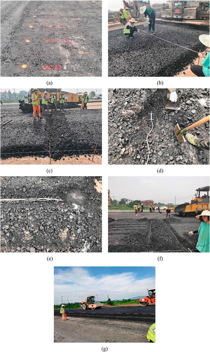
Figure 1. Temperature sensor burial process: (a) determination of sensor positions; (b) loose-packing of the mix; (c) channel cutting; (d) buried sensors; (e) coverage with fines; (f) filling of potholes; and (g) road crushing.

2.5.3 Data acquisition instrument wiring

① Guide the cables to the roadside data collector through the excavated trench;

② Connect the numbered cables to the corresponding interfaces of the data acquisition instrument and check the sensor signal output;

③ After all sensors are buried and connected to the data acquisition instrument, place the instrument in a cool and sheltered location to protect it from rain;

④ Bury the sensor cables at the roadside with soil and set up warning signs after compaction.

2.5.4 Equipment inspection and calibration

To ensure data accuracy, the operation of the equipment should be promptly checked after the sensor is connected to the data collector, and the data collector should be calibrated. The equipment operation status inspection should include checks on the sensor survival status, cable connections, data collector functionality, sensor location, and numbering, among others. The calibration of the data acquisition instrument is performed to improve measurement accuracy and reduce instrument error. It mainly includes the following steps: ①Turn on the calibration switch and determine the instrument reading based on the sensitivity factor. ②Adjust the potentiometer on the instrument dial to achieve a reading of approximately 10,000/K.

3 Characterization of the spatial and temporal distribution of high temperature fields in asphalt pavement

Research shows that rutting deformation in asphalt pavement mainly occurs during the high-temperature period in summer. Therefore, this section selects 31 August 2021 as the representative day of the high-temperature period to analyze the high-temperature field of the road surface.

3.1 Variation of meteorological factors with time

The variation of solar radiation intensity Q, temperature T, and wind speed v over time t on the representative day during the high-temperature period is shown in Figure 2. The sampling interval is 15 min.

Figure 2

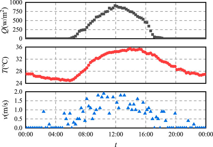
Figure 2. Patterns of change in meteorological factors over time.

As shown in Figure 2:

① The solar radiation intensity shows a roughly symmetrical normal distribution over time, peaking at approximately 12 p.m., with a maximum daily solar radiation intensity of 911 w/m².

② The temperature varies with time in a roughly sinusoidal curve, experiencing a cooling–warming–cooling process throughout the day. The highest temperature of 35.5°C occurs at approximately 2 p.m., while the lowest temperature of 25.5°C occurs at approximately 6:00 am. It takes approximately 9 h to rise from the trough to the peak, while it takes more than 15 h to fall from the peak to the trough, which shows that the heat absorption rate of the atmosphere is higher than the heat release rate. In addition, the peak temperature lags slightly behind the peak solar radiation intensity, due to the time required for air conduction and convection.

③ The wind speed showed no clear regularity over time, with a wide range of fluctuations. The highest wind speed on the representative day was 2.0 m/s, which appeared at approximately 11 p.m.

3.2 Change rule of pavement temperature with time

The pattern of change in pavement temperature over time for the high-temperature representative day is shown in Figure 3, and the corresponding characteristic temperatures are listed in Table 1.

Figure 3

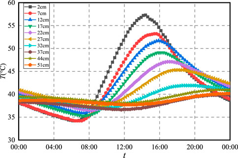
Figure 3. Pavement structure temperature change rule with time.

Table 1

Table 1. Timing of characteristic temperatures at different depths of the pavement.

As shown in Figure 3 and Table 1:

① The temperature change trend of each structural layer of the flexible asphalt pavement follows a similar pattern, with a sinusoidal curve. The curve can be roughly divided into two stages: warming and cooling. After sunrise, solar radiation increases, causing the road surface to absorb heat, and the temperature rises rapidly, peaking at approximately 14:30. As the radiation intensity gradually decreases, the heat from the road surface dissipates from the inside to the outside, and the structural temperature gradually decreases until the early morning. In addition, the pavement structure warmed up for approximately 8 h and cooled down for approximately 16 h, which shows that the heat absorption rate of asphalt pavement is much higher than the heat release rate.

② As the depth increases, the peak and valley points of the pavement temperature become more delayed. This is due to the time required for heat conduction along the depth of the road surface. Environmental factors have less immediate impact on the deeper layers of the pavement structure. When the depth of the structure is less than 37 cm, an increase of 1 cm causes a delay of approximately 8 min for the peak and approximately 5 min for the valley. However, when the depth is more than 37 cm, the temperature of the pavement structure is basically maintained at approximately 40°C, and the timing of the extreme values becomes irregular, with less noticeable changes.

3.3 Change rule of pavement temperature along depth

The shallow daily minimum temperature of the road surface usually occurs at 6 a.m., while the daily maximum temperature is reached at approximately 3 p.m. The intensity of solar radiation peaks at approximately 12 p.m. Therefore, the entire day from 12 a.m. to 12 a.m. is divided into 3-h intervals.

The variation in pavement temperature (T) with depth (H) at different times during the high-temperature representative day is shown in Figure 4, and the characteristic temperatures are shown in Table 2.

Figure 4

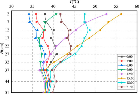
Figure 4. Temperature change rule along the vertical direction of the pavement surface.

Table 2

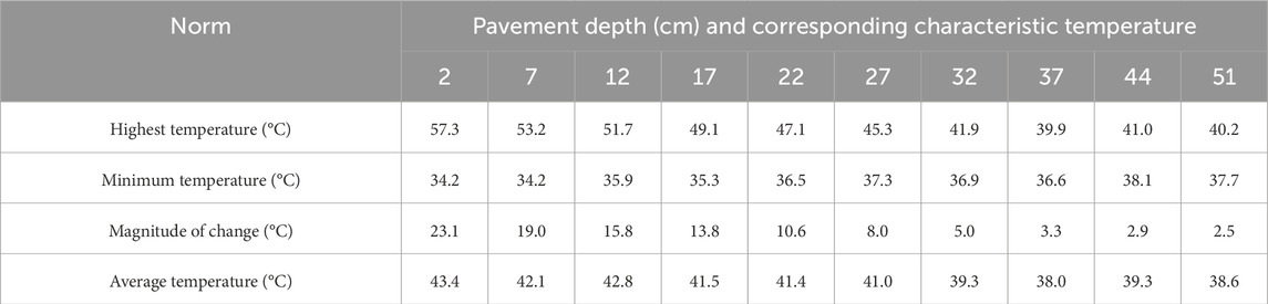
Table 2. Characteristic temperatures of pavement at different depths.

As shown in Figure 4 and Table 2:

① The diurnal maximum temperature within the pavement structure exhibits a progressive decrease followed by stabilization as depth increases. Beyond the critical depth of 32 cm, maximum temperatures stabilize at approximately 40°C. In contrast, the daily minimum temperature exhibits a slight upward trend with depth, with thermal fluctuations confined to a 5°C amplitude. Both the temperature fluctuation magnitude and maximum temperature profiles follow a similar pattern, initially decreasing and then stabilizing with depth. This thermal stratification establishes a critical boundary at 32 cm: above this depth, environmental factors dominate, leading to significant cooling rates and thermal amplitude variations; below this depth, temperature stability increases due to reduced environmental influence and greater reliance on geothermal equilibrium.

② Distinct thermal regimes govern heat transfer across the diurnal phases:

00:00–06:00 h: Heat dissipates outward from deeper pavement layers, establishing a stable thermal gradient with temperatures marginally increasing at greater depths. 09:00 h: Surface temperatures rise sharply under solar radiation, while subsurface layers retain thermal inertia, maintaining near-uniform temperatures. 09:00–15:00 h: Sustained solar radiation drives heat downward, creating a temperature gradient that decreases gradually with depth before stabilizing. Post-18:00 h: Surface radiative cooling initiates rapid heat dissipation, generating a thermal inversion where temperatures initially rise before declining with increasing depth.

4 Characterization of the spatial and temporal distribution of low-temperature field in asphalt pavement

Since rutting deformation rarely occurs in the low-temperature period, this section of the study will focus on the changes in the pavement temperature field during the high-temperature period for comparative verification. The analysis under low-temperature conditions will be brief, mainly serving as a means of validating the data collected during the high-temperature period.

4.1 Change rule of pavement temperature with time

4.1.1 Daily variation

To improve the completeness of the research, a representative low-temperature day (29 December 2021) is selected to characterize the low-temperature field of the pavement structure.

Figure 5 reflects the temperature fluctuations over 1 day during the low-temperature period, and the main patterns are as follows.

① As the depth of the pavement increases, the influence of air temperature on the pavement temperature decreases. Below 32 cm from the road surface, the daily temperature remains basically unchanged, and the temperature curve is basically a flat line;

② The temperature of structural layers at different depths is affected by environmental factors and there is a hysteresis effect. With the deepening of the layer, the time at which the maximum temperature occurs is gradually delayed;

③ The temperature curve shows obvious daily fluctuations, with the highest temperature usually occurring at approximately 1:30 p.m. and the lowest at approximately 7:30 a.m. The temperature of the structural layers reaches equilibrium and stabilizes at approximately 9:00 a.m. The temperature increases faster as it gets closer to the road surface until it reaches equilibrium again at approximately 5:30 p.m.

Figure 5

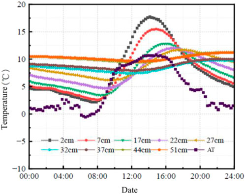
Figure 5. Daily patterns of pavement structural temperatures.

4.1.2 Monthly variation

The data for December 2021 was selected to study the low-temperature monthly variations, as the presence of more rainfall days during the low-temperature period could affect the temperature field.

Figure 6 reflects the fluctuation situation in January of the low-temperature period, and the main laws are as follows:

① The temperature curve exhibits periodic fluctuations influenced by the day–night temperature difference and solar radiation changes. Approximately 32 cm below the road surface, the temperature curve shows up and down fluctuations. Beyond 32 cm, the daily temperature basically remains stable, and the temperature curve becomes nearly flat.

Figure 6

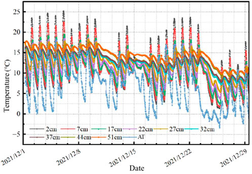
Figure 6. Monthly patterns of pavement structural temperatures.

The lowest temperature of the structural layer was 0.7°C at the road surface.

③ The temperature within the structural layer is generally at a low level, below 20°C most of the time. There is a large temperature difference between day and night in most weather conditions, and the maximum temperature difference at the road surface reaches 45.4°C, while the maximum temperature difference at the bottom reaches 14.6°C.

④ The lowest temperature of the structural layer occurred at the road surface. At this time, the temperatures at depths 7, 12, 17, 22, 27, 32, 37, 44, and 51 cm from the road surface were 13, 15.1, 14.5, 16, 17.3, 18.2, 18.4, 19.8°C, and 19.7°C respectively.

4.2 Change rule of pavement temperature along depth

The curves of temperature variation with depth within the pavement structure at different times are shown in Figure 7.

Figure 7

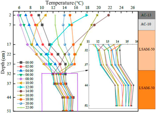
Figure 7. Temperature change rule along the vertical direction of the pavement surface.

As shown in Figure 7, the temperature difference within the pavement structure decreases with increasing depth, with the lowest and highest temperatures usually occurring at the pavement surface. The most significant temperature changes occur at the pavement surface. Comparing with the results in Section 3, the temperature change within the pavement structure is more rapid in summer than in winter. Above 32 cm from the pavement surface, the temperature tends to decrease with increasing depth during the hot summer and increase during the cold winter months. However, whether during the high- or low-temperature periods, when the depth exceeds 32 cm, the daily temperature basically remains unchanged, and the temperature curve becomes nearly. Therefore, areas deeper than 30 cm are designated as temperature-insensitive zones.

5 Modeling of high-temperature temperature field prediction in asphalt pavements

5.1 Temperature field prediction model parameter selection

The main parameters affecting pavement temperature distribution are air temperature and solar radiation intensity. Other environmental factors, such as wind speed, rainfall, and humidity, mainly affect the pavement temperature field under specific weather conditions and can be reflected by air temperature and solar radiation intensity. Therefore, pavement temperature (T_H) can be expressed as a composite function of air temperature (T_a), solar radiation intensity (Q), and pavement depth (H), i.e., T_H = f (T_a,Q,H).

5.1.1 Cumulative and lagged impacts of environmental factors

The analysis clearly shows that the effects of temperature and solar radiation on pavement temperature distribution are cumulative and exhibit a lag. Pavement temperatures are influenced not only by current environmental factors but also by the previously experienced temperature and solar radiation history.

To study the cumulative effect of environmental factors on the structural temperature of asphalt pavements, the average values of air temperature and solar radiation intensity over the first n hours were calculated, and their respective correlations with the structural temperature of the pavements were analyzed as shown in Figure 8.

Figure 8

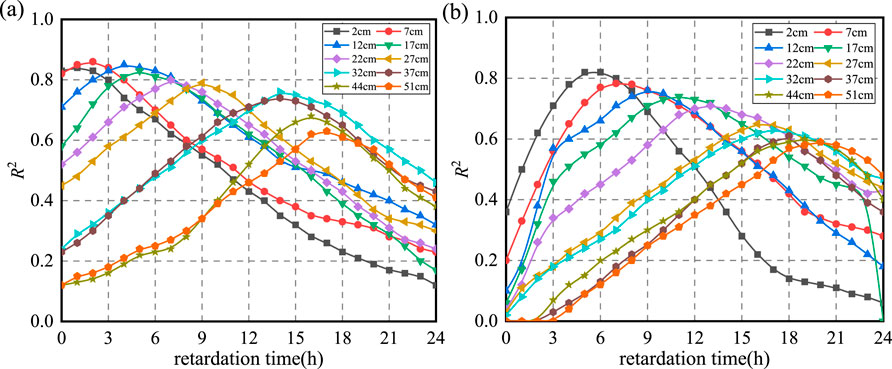
Figure 8. Correlation of pavement temperature with meteorological factors: (a) cumulative temperature; (b) cumulative solar radiation.

Figure 8 illustrates that the maximum correlation between structural temperature and the cumulative average air temperatures over 1 h, 2 h, 4 h, 5 h, 7 h, 9 h, 12 h, 14 h, 16 h, and 17 h was observed at pavement depths of 2 cm, 7 cm, 12 cm, 17 cm, 22 cm, 27 cm, 32 cm, 37 cm, 44 cm, and 51 cm, respectively. Similarly, the highest correlations with the cumulative mean solar radiation over 6 h, 7 h, 9 h, 11 h, 13 h, 16 h, 17 h, 18 h, 19 h, and 20 h were identified.

To investigate the hysteresis effect of environmental factors, the average air temperature and solar radiation intensity over the preceding m hours were computed, and their correlations with pavement structure temperature were analyzed. The results are presented in Figure 9.

Figure 9

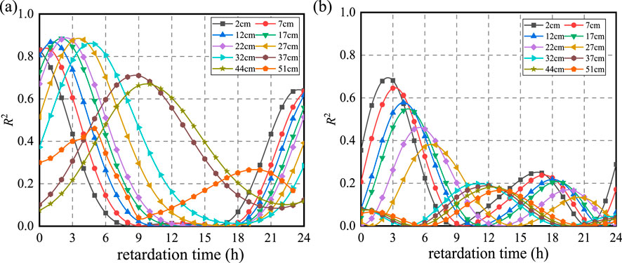
Figure 9. Correlation of pavement temperature with meteorological factors: (a) lagging temperature; (b) lagging solar radiation.

Figure 9 demonstrates that pavement temperatures at depths of 2 cm, 7 cm, 12 cm, 17 cm, 22 cm, 27 cm, 32 cm, 37 cm, 44 cm, and 51 cm exhibit the highest correlation with air temperatures at lag times of 0 h, 1 h, 1 h, 2 h, 2 h, 4 h, 5 h, 8 h, 10 h, and 10 h, respectively. Similarly, the highest correlations with solar radiation are observed at lag times of 3 h, 3 h, 4 h, 4 h, 4 h, 4 h, 4 h, 4 h, 4 h, 4 h, 4 h, 4 h, 3 h, 3 h, 3 h, 4 h, 4 h, 4 h, 5 h, 7 h, 10 h, 12 h, 12 h, and 13 h.

5.1.2 Effect of pavement depth

Existing studies have shown that the distribution pattern of pavement temperature along the depth direction can be approximated as a cubic polynomial (Li et al., 2018). To verify this conclusion, the measured temperature data were used as the basis for fitting the temperature-depth curves using second-, third-, and fourth-degree polynomials, respectively, and the relevant parameters are shown in Figure 10.

Figure 10

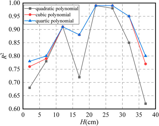
Figure 10. Changes in correlation coefficients of fitted curves with depth.

As shown in Figure 10, the correlation coefficient of the pavement temperature–depth relationship fitted using a cubic polynomial is significantly higher than that of a quadratic polynomial, whereas the degree of correlation does not improve significantly after increasing it further to a quadratic polynomial. Therefore, it is reasonable to use a cubic polynomial to model the temperature distribution pattern along the road surface direction.

In addition, the influence of environmental factors on pavement temperature distribution gradually weakens with increasing depth. Therefore, the product of air temperature and solar radiation intensity, combined with the depth of the pavement, is introduced into the prognostic model to account for the varying degrees of environmental impact on the structural temperature at different depths.

5.2 Temperature field prediction model fitting and building

Based on the asphalt pavement temperature field prediction model proposed by Prof. Sun Lijun (Li et al., 2018), as shown in Equation 1, the model was refined by combining the parameters in the study that best reflect the cumulative and hysteretic effects of environmental factors on pavement temperature. By replacing the corresponding parameters in the original model, an improved pavement temperature field prediction model was obtained, as shown in Equation 2.

${\theta }_p=p_1+\left(p_2{\theta }_{a5}+p_3{Q_5}^2\right)+H\left(p_4{\theta }_a+p_{5}Q\right)+\left(p_{6}H+p_7{H}^2+p_8{H}^3\right),(1)$

where θ_p is the temperature of a certain depth of the leached road surface, °C; θ_a is the front gas temperature, °C; Q is the radiation intensity of the front sun, kW·m^-2; θ_a5 is the average gas temperature for the first 5 h, °C; Q₅ is the mean solar radiation intensity for the first 5 h, kW·m^-2; H is the depth of road surface, cm; and p₁∼p₈ is the return system to be determined.

$T_H=a_1+a_2{T}_{l1}+a_3{Q}_{l6}+H\left(a_4{T}_0+a_5{Q}_{z3}\right)+\left(a_{6}H+a_7{H}^2+a_8{H}^3\right),(2)$

where T_H is pavement temperature at depth H, °C; T_l1 is the mean value of cumulative 1-h temperature, °C; Q_l6 is the mean value of cumulative 6-h solar radiation intensity, Kw/m²; T₀ is current air temperature, °C; Q_z3 is the lagged 3-h solar radiation intensity, Kw/m²; H is the pavement depth, cm; a₁∼a₈ are regression coefficients.

The least squares method is used for multiple regression analysis of air temperature, solar radiation intensity, pavement depth, and the corresponding pavement temperature, and the fitting results are shown in Table 3. Substituting each parameter in Table 3 into Equation 2, the prediction model for the pavement temperature field during the high-temperature period in the Wuwei area is obtained, as shown in Equation 3.

$T_p=1.86+0.076T_{l1}+0.001Q_{l6}+H\left(0.99T_0+0.027Q_{z3}\right)+0.016H+0.010H^2-0.001H^3(3)$

Table 3

Table 3. Temperature field prediction model regression coefficients.

The model was used to calculate the pavement temperature at different depths, and the calculated and measured curves are shown in Figure 11, while the correlation between the two is shown in Figure 12.

Figure 11

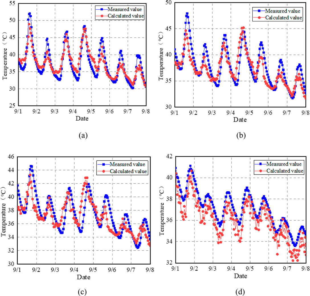
Figure 11. Correlation between calculated and measured pavement temperature curves: (a) 2 cm; (b) 12 cm; (c) 22 cm; (d) 32 cm.

Figure 12

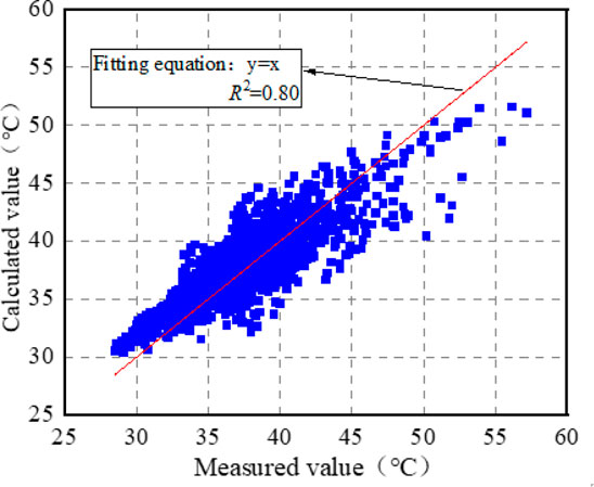
Figure 12. Correlation between calculated and measured pavement temperatures.

From Figures 11, 12, it can be seen that the temperature curves of different depths of the pavement, calculated using the prediction model (Equation 3), are relatively close to the measured curves. The calculated values are uniformly distributed in the vicinity of the 45-degree contour, with a correlation of approximately 80%, which indicates that this model can more accurately characterize the temperature distribution field of the asphalt pavement.

5.3 Predictive modeling of maximum pavement temperature

The peak pavement temperature is closely related to the peak air temperature and the peak solar intensity. Therefore, the maximum air temperature T_amax and the maximum solar radiation intensity Q_max are introduced into Equation 3 to establish the model for estimating the daily maximum temperature. The formula is shown in Equation 4, and the corresponding parameters are subjected to multiple regression analysis, with the fitting results shown in Table 4.

$T_{H\text{ma}\mathrm{x}}=m_1+m_2{T}_{a\max }+m_3{Q}_{\text{ma}\mathrm{x}}^2+H\left(m_4{T}_{a\max }+m_5{Q}_{\max }\right)+\left(m_{6}H+m_7{H}^2+m_8{H}^3\right),(4)$

Table 4

Table 4. Parameters related to daily maximum temperature prediction model.

where T_Hmax is the daily maximum temperature at depth H, °C; T_amax is the daily maximum temperature, °C; Q_max is the daily maximum solar radiation intensity, kW/m²; and m₁∼m₈ are regression coefficients.

By substituting each parameter from Table 4 into Equation 4, the model for predicting the daily maximum temperature of asphalt pavement during the high-temperature season in the Wuhui area is obtained.

$T_{H\max }=18.2+0.969T_{a\max }+0.010{Q_{\max }}^2+H\left(-0.001T_{a\max }-0.147Q_{\max }\right)-0.245H(5)$

Equation (5) was used to calculate the maximum daily temperature of the flexible base asphalt pavement, and the correlation between the calculated and measured values is shown in Figure 13.

Figure 13

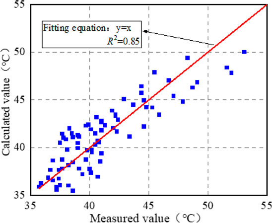
Figure 13. Correlation between calculated and measured daily maximum pavement temperatures.

As shown in Figure 13, the correlation between the calculated and measured values of the daily maximum temperature reaches 85%, indicating that the model can accurately characterize the changes of the daily maximum temperature of asphalt pavement with environmental factors.

5.4 Predictive modeling of minimum pavement temperature

The daily minimum temperature of the pavement generally occurs at night or in the early morning when there is no solar radiation, and the distribution along the depth direction is not as complicated as the daily maximum temperature. Therefore, the prediction model for the daily minimum temperature of the pavement can be expressed by Equation 6, and the related parameters are shown in Table 5.

$T_{H\min }=n_1+n_2{T}_{a\min }+\left(n_{3}H+n_4{H}^2\right),(6)$

Table 5

Table 5. Parameters related to daily minimum temperature prediction model.

where T_Hmin is the daily minimum mixing at pavement depth H, °C; T_amin is the daily minimum temperature, °C; and n₁∼n₄ are regression coefficients to be determined.

By substituting each parameter from Table 5 into Equation 6, the model for predicting the daily minimum temperature of asphalt pavement during the high-temperature season in the Wuhui area is obtained.

$T_{P\min }=0.007+0.946T_{a\min }+0.141H-0.001H^2+0.354T_m(7)$

Equation 7 was used to calculate the daily minimum temperature of the pavement, and the correlation between the calculated and measured values is shown in Figure 14.

Figure 14

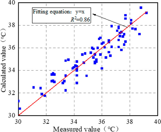
Figure 14. Correlation between predicted and measured daily minimum temperature of road surface.

As shown in Figure 14, the correlation between the calculated and measured daily minimum temperatures of the pavement reaches 86%, indicating that the model can accurately characterize the changes of the daily minimum temperature of asphalt pavement with environmental factors.

6 Application of temperature field prediction model

Rutting deformation in asphalt pavement increases exponentially with rising temperatures, while pavement temperature changes periodically with time and alternately with the depth of positive and negative gradient distribution. Accurately understanding the spatial and temporal distribution of pavement temperature and its impact on rutting deformation is a key problem for the rutting-resistant design of LSAM-50 pavements. The application of a long-term temperature prediction model to calculate the structural layer temperature can effectively solve this problem.

The temperature of each layer of the pavement structure is shown in Table 6. Considering the influence of the maximum daily temperatures of 30°C, 35°C, and 40°C on the rutting deformation of LSAM-50 flexible base layer asphalt pavement, the highest temperature prediction model of the pavement was used an example. Based on the test results of Section 3, the maximum solar radiation intensity Qmax was found to be 0.9 kW/m². The temperature at the top surface of each layer was then calculated by substituting the corresponding depth values into Equation 3, with the top surface temperature as the temperature for each layer.

Table 6

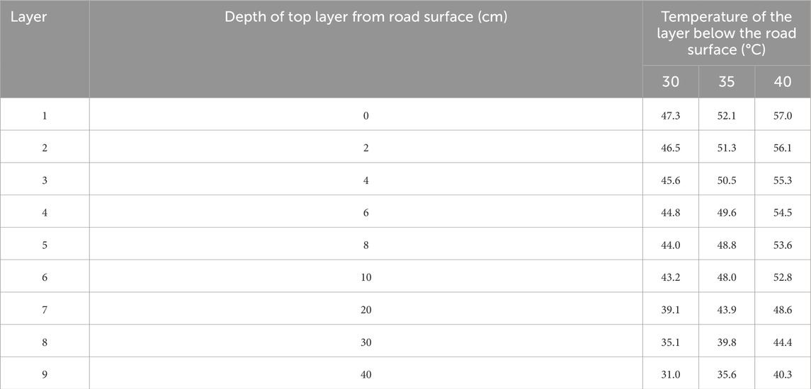
Table 6. Temperature of each layer of pavement structure.

7 Conclusion

(1) The test section was introduced based on the project overview, including on-site meteorological parameters and pavement temperature data acquisition equipment. In addition, the sensor burial program for measuring pavement temperature was presented.

(2) The change in meteorological factors over time during the high-temperature period in summer was analyzed. The results show that the intensity of solar radiation is symmetrically distributed at approximately 12 o’clock, reaching its peak at approximately noon. The temperature changes over time follow a sinusoidal pattern, with the warming rate exceeding the cooling rate. The peak temperature generally occurs at approximately 2 p.m., lagging behind the peak of solar radiation.

(3) The distribution characteristics of asphalt pavement temperature field with time and depth were studied. The results show that the temperature change trend is basically the same across different structural layers, following a cooling–warming–cooling pattern throughout the day, and the warming rate is much higher than the cooling rate. As depth increases, the peak temperature of the pavement lags further, with each 1 cm increase in depth causing a delay of approximately 8 min at the peak and 5 min at the valley. The maximum daily pavement temperature and the magnitude of temperature change in the depth direction decrease and eventually stabilize, with the critical depth occurring at approximately 32 cm.

(4) Based on the cumulative and lagging effects of environmental factors on the pavement structure temperature, combined with the distribution characteristics of pavement temperature along the depth, a temperature field prediction model for the flexible base layer asphalt pavement structure during the summer high-temperature period was developed, using the model proposed by Prof. Sun Lijun of Tongji University. The model shows a correlation of 80%.

(5) The prediction models for the daily maximum temperature and minimum temperatures of flexible base layer asphalt pavement during the high-temperature period were established, with correlation coefficients above 80%.

(6) The application of the temperature field prediction model was carried out as an example of the maximum pavement prediction model, and the temperatures within each structural layer of the LSAM-50 pavement were calculated.

It should be emphasized that these studies are based on a specific region, and regional differences will inevitably affect the generalizability of the model. This limitation can be resolved by introducing regional correction coefficients.

Data availability statement

The original contributions presented in the study are included in the article/supplementary material; further inquiries can be directed to the corresponding authors.

Author contributions

YB: data curation and writing – review and editing. MM: investigation and writing – review and editing. MG: writing – original draft. WW: writing – review and editing. TD: formal analysis and writing – review and editing. CQ: methodology and writing – review and editing. DY: formal analysis and writing – review and editing. YJ: resources, supervision, and writing – review and editing. HS: writing – original draft.

Funding

The author(s) declare that no financial support was received for the research and/or publication of this article.

Conflict of interest

Authors YB, MM, and CQ were employed by Shandong high-speed Group Co., Ltd. Authors TD and DY were employed by Shandong Transportation Planning and Design Institute Group Co., Ltd.

The remaining authors declare that the research was conducted in the absence of any commercial or financial relationships that could be construed as a potential conflict of interest.

Generative AI statement

The author(s) declare that no Generative AI was used in the creation of this manuscript.

Publisher’s note

All claims expressed in this article are solely those of the authors and do not necessarily represent those of their affiliated organizations, or those of the publisher, the editors and the reviewers. Any product that may be evaluated in this article, or claim that may be made by its manufacturer, is not guaranteed or endorsed by the publisher.

References

Adwan, I., Milad, A., Memon, Z. A., Widyatmoko, I., Zanuri, N. A., Memon, N. A., et al. (2021). Asphalt pavement temperature prediction models: a review. Appl. Sci.-Basel 11 (9), 3794. doi:10.3390/app11093794

CrossRef Full Text | Google Scholar

Aliha, M. R. M., Fazaeli, H., Aghajani, S., and Nejad Moghadas, F. (2015). Effect of temperature and air void on mixed mode fracture toughness of modified asphalt mixtures. Constr. Build. Mater. 95, 545–555. doi:10.1016/j.conbuildmat.2015.07.165

CrossRef Full Text | Google Scholar

Barber, E. S. (1957). Calculation of maximum pavement temperatures from weather reports. Highw. Res. Board Bull. 168. Available online at: https://api.semanticscholar.org/CorpusID:135835144

Google Scholar

Bi, Y., Mu, M., Zeng, L., Ding, T., Qian, C., Yu, D., et al. (2024). Development and road performance verification of aggregate gradation for large stone asphalt mixture. Materials 17 (23), 5712. doi:10.3390/ma17235712

PubMed Abstract | CrossRef Full Text | Google Scholar

Bosscher, P. J., Bahia, H. U., Thomas, S., and Russell, J. S. (1998). Relationship between pavement temperature and weather data: Wisconsin field study to verify superpave algorithm. Transp. Res. Rec. 1609 (1), 1–11. doi:10.3141/1609-01

CrossRef Full Text | Google Scholar

Boussabnia, M. M., Perraton, D., Lamothe, S., Di Benedetto, H., Proteau, M., and Pouteau, B. (2023). Temperature effect on fatigue behavior of high-modulus asphalt concrete (HMAC). Constr. Build. Mater. 409, 134006. doi:10.1016/j.conbuildmat.2023.134006

CrossRef Full Text | Google Scholar

Cheng, H. L., Liu, J. N., Sun, L. J., et al. (2021). Critical position of fatigue damage within asphalt pavement considering temperature and strain distribution. Int. J. Pavement Eng. 22 (14), 1773–1784. doi:10.1080/10298436.2020.1724288

CrossRef Full Text | Google Scholar

Crevier, L. P., and Delage, Y. (2001). METRo: a new model for road-condition forecasting in Canada. J. Appl. Meteorology Climatol. 40 (11), 2026–2037. doi:10.1175/1520-0450(2001)040<2026:manmfr>2.0.co;2

CrossRef Full Text | Google Scholar

Diefenderfer, B. K., Al-Qadi, I. L., and Diefenderfer, S. D. (2006). Model to predict pavement temperature profile: development and validation. J. Transp. Eng. 132 (2), 162–167. doi:10.1061/(asce)0733-947x(2006)132:2(162)

CrossRef Full Text | Google Scholar

Fan, X. Y., Lv, S. T., Ge, D. D., Liu, C. C., Peng, X. H., and Ju, Z. H. (2022). Time-temperature equivalence and unified characterization of asphalt mixture fatigue properties. Constr. Build. Mater. 359, 129118. doi:10.1016/j.conbuildmat.2022.129118

CrossRef Full Text | Google Scholar

Hamed, M., and Makki, M. S. (2011). Influence of ambient temperature on stiffness of asphalt pavin materials. J. Eng. 17 (05), 1090–1108. doi:10.31026/j.eng.2011.05.05

CrossRef Full Text | Google Scholar

Hermansson, Å. (2001). Mathematical model for calculation of pavement temperatures: comparison of calculated and measured temperatures. Transp. Res. Rec. 1764 (1), 180–188. doi:10.3141/1764-19

CrossRef Full Text | Google Scholar

Im, S., Kim, Y. R., and Ban, H. (2013). Rate- and temperature-dependent fracture characteristics of asphaltic paving mixtures. J. Test. Eval. 41 (2), 257–268. doi:10.1520/jte20120174

CrossRef Full Text | Google Scholar

Jiang, J. W., Dong, Q., Ni, F. J., and Yu, H. (2018). Development of permanent deformation master curves of asphalt mixtures by load-temperature superposition. J. Mater. Civ. Eng. 30 (6), 04018098. doi:10.1061/(asce)mt.1943-5533.0002300

CrossRef Full Text | Google Scholar

Kondo, Y., and Miura, Y. (1976). “On the prediction of temperature in pavement structures,” in Proceedings of the Japan society of civil engineers (Japan Society of Civil Engineers), &gt;250 123–132. doi:10.2208/jscej1969.1976.250_123

CrossRef Full Text | Google Scholar

Kong, X. M., Liu, Y. L., Zhang, Y. R., Zhang, Z. l., Yan, P. y., and Bai, Y. (2014). Influences of temperature on mechanical properties of cement asphalt mortars. Mater. Struct. 47 (1-2), 285–292. doi:10.1617/s11527-013-0060-2

CrossRef Full Text | Google Scholar

Kršmanc, R., Slak, A. Š., and Demšar, J. (2013). Statistical approach for forecasting road surface temperature. Meteorol. Appl. 20 (4), 439–446. doi:10.1002/met.1305

CrossRef Full Text | Google Scholar

Li, Q., Ma, X., Ni, F. J., and Li, G. F. (2015). Characterization of strain rate and temperature-dependent shear properties of asphalt mixtures. J. Test. Eval. 43 (5), 20140056. doi:10.1520/jte20140056

CrossRef Full Text | Google Scholar

Li, Y., Liu, L. P., and Sun, L. J. (2018). Temperature predictions for asphalt pavement with thick asphalt layer. Constr. Build. Mater. 160, 802–809. doi:10.1016/j.conbuildmat.2017.12.145

CrossRef Full Text | Google Scholar

MOT (2004). Technical specifications for construction of highway asphalt pavements, JTG F40-2004.

Google Scholar

MOT (2011). Test procedures for bitumen and bituminous mixtures in highway engineering, JTG E20-2011.

Google Scholar

MOT (2017). Design specifications for highway asphalt pavements, JTG D50-2017.

Google Scholar

Pérez-Jiménez, F., Botella, R., Moon, K. H., and Marasteanu, M. (2013). Effect of load application rate and temperature on the fracture energy of asphalt mixtures. Fenix and semi-circular bending tests. Constr. Build. Mater. 48, 1067–1071. doi:10.1016/j.conbuildmat.2013.07.084

CrossRef Full Text | Google Scholar

Qi, L., Yu, B. Y., Zhao, Z. H., and Zhang, C. S. (2023). Temperature field analytical solution for OGFC asphalt pavement structure. Coatings 13 (7), 1172. doi:10.3390/coatings13071172

CrossRef Full Text | Google Scholar

Qian, G. P., Yang, H., Li, X., Yu, H. A., Gong, X. B., and Zhou, H. Y. (2021). A unified strength model of asphalt mixture considering temperature effect. Front. Mater. 8, 8. doi:10.3389/fmats.2021.754187

CrossRef Full Text | Google Scholar

Stukhlyak, P. D., Buketov, A. V., Panin, S. V., Maruschak, P. O., Moroz, K. M., Poltaranin, M. A., et al. (2015). Structural fracture scales in shock-loaded epoxy composites. Phys. Mesomech. 18, 58–74. doi:10.1134/s1029959915010075

CrossRef Full Text | Google Scholar

Williamson, R. (1972). Effects of environment on pavement temperatures. Intl Conf. Struct. Des. Proc.

Google Scholar

Yang, X. H., Shang, J., Yin, A. Y., Yang, S. F., and Ye, Y. (2010). “Effect of temperature and wheel loading on rutting deformatio of asphalt mixture,” in 10th asia-pacific conference on engineering plasticity and its applications (AEPA), world scientific publ Co pte Ltd, wuha (PEOPLES R CHINA), 492–496.

Google Scholar

Yin, Z., Hadzimustafic, J., Kann, A., and Wang, Y. (2019). On statistical nowcasting of road surface temperature. Meteorol. Appl. 26 (1), 1–13. doi:10.1002/met.1729

CrossRef Full Text | Google Scholar

Zhang, J., Fwa, T., Tan, K., and Shi, X. (2003). Model for nonlinear thermal effect on pavement warping stresses. J. Transp. Eng. 129 (6), 695–702. doi:10.1061/(asce)0733-947x(2003)129:6(695)

CrossRef Full Text | Google Scholar