Development of defect localization method for perforated carbon-fiber-reinforced plastic specimens using finite element method and graph neural network

In this study, we propose a novel defect localization method that integrates the graph neural network (GNN) with the finite element method (FEM) to estimate the three-dimensional location of defects in perforated carbon-fiber-reinforced plastic (CFRP) interstage structures. Specifically, the model uses distributions of the sum of principal stresses on the surface (DSPSS) to predict the three-dimensional location of defects. FEM is employed to simulate tensile loading conditions and generate stress distribution data using Teflon sheets to represent predefined delaminations. These distributions serve as inputs to the graph attention network (GAT), which classifies defect positions into 19 categories. The proposed method achieved a macro-averaged F1-score of 61% and accurately predicted both the insertion layers and planar positions of defects.

1 Introduction

CFRP is a composite material composed of carbon fibers embedded in a polymer resin matrix. Owing to its exceptionally high specific strength and stiffness, CFRP is widely utilized in aerospace structures and automotive components. In particular, it has become indispensable in the aerospace industry, where both lightweight and high reliability are essential. Its applications include interstage structures in space launch vehicles, satellite fairings, and external structures of fuel tanks. Notably, more than 50% of the airframe structure in Boeing 787 incorporates CFRP (Ning et al., 2016). Typically, CFRP is fabricated by laminating prepregs—unidirectionally reinforced sheets, which provide high strength and stiffness along a specific direction (Christensen, 2012). As its use continues to expand, defect detection during both the manufacturing and operational phases has become a critical issue (Kiefel et al., 2015; Stoessel et al., 2011). However, damage modes in laminated CFRP are often complex, including delamination, fiber breakage, and matrix cracking. Therefore, high-efficiency and high-accuracy damage evaluation techniques are required. Conventionally, nondestructive testing (NDT) methods such as ultrasonic inspection (Scarponi and Briotti, 2000), X-ray radiography (Sultan et al., 2011), and tap testing (Mills et al., 2020) have been utilized. NDT enables the evaluation of material integrity without causing destruction, and although traditionally applied to metals such as steel and aluminum, recent developments have extended its use to composite materials including CFRP. Since internal damage such as delamination or fiber fracture is often not observable externally, NDT plays an essential role in ensuring structural safety (Caminero et al., 2019; Pirinu and Panella, 2021).

Radiographic inspection leverages the penetrative properties of X or $\gamma$ rays to detect internal inhomogeneities or defects. This method excels at identifying volumetric defects and can provide objective information about defect type, shape, and size. For example, Dilonardo et al. applied high-resolution X-ray computed tomography (CT) to CFRP laminates and sandwich structures widely used in aircraft, successfully visualizing voids and fiber misalignments (Dilonardo et al., 2020). Bagale et al. demonstrated the utility of X-ray transmission in evaluating long-term moisture thermal degradation in CFRP, enabling the noncontact and quantitative assessment of internal changes (Bagale and Bhat, 2020). Whereas advanced X-ray CT systems enable the three-dimensional imaging, conventional radiography techniques are generally limited to two-dimensional projection views, and challenges remain regarding spatial setup, safety protocols, and equipment costs.

Ultrasonic testing involves sending ultrasonic pulses into a target material and detecting reflections from internal flaws. It allows single-sided inspection and provides through-thickness information, with relatively fewer safety concerns than radiographic methods. Lee et al. developed a noncontact ultrasonic system using laser-generated guided waves and air-coupled sensors for real-time defect detection during CFRP fabrication, and identified the attenuation of high-frequency wave components in delaminated regions (Lee et al., 2006). Joas et al. proposed an automated method using airborne ultrasonics to inspect CFRP pipes, demonstrating its feasibility for mass-produced components (Joas et al., 2019). Recent advancements include hybrid methods and image fusion to further enhance defect discrimination accuracy (Pohl, 2016; Torbali et al., 2023; Chen et al., 2012). Nonetheless, limitations include their lower resolution than radiographic techniques and variability in results depending on couplant use and operator skill.

Tap testing involves striking the surface of a structure with a rigid rod or hammer and evaluating sound differences either audibly or via sensors to infer internal defects. This method is widely used as a practical screening technique for large or complex structures, such as CFRP panels and rockets, owing to its operational efficiency and rapid assessment capability (Cawley and Adams, 1987). It requires minimal equipment and is well-suited for rapid field inspection. However, this method relies heavily on auditory perception and experience, which compromises objectivity and repeatability. In noisy environments or for complex geometries, defect localization becomes less reliable. In practice, tap testing is often used for initial diagnostics, followed by higher-precision NDT where anomalies are found.

In addition to the above techniques, infrared thermography has been explored as an alternative damage evaluation technique (Keo et al., 2015; Yang et al., 2013; Ishikawa et al., 2013; Fang et al., 2021; Ishikawa et al., 2012; Kidangan et al., 2021; Wu et al., 2018; Popow and Gurka, 2020). In this technique, the infrared radiation emitted from an object’s surface is measured using infrared (IR) sensors and converted into temperature distribution data. Compared with other methods, IR thermography requires no contact media, entails smaller safety and cost burdens, and enables faster measurements. However, the accurate interpretation of results requires considerable expertise, making the method prone to variability and operator dependence. Recent developments have employed infrared stress measurement, by which the distributions of the sum of principal stresses on the surface (DSPSS) are calculated from thermal variations (Qiu et al., 2022). This technique can achieve a resolution of approximately 1 MPa in mild steel and requires only basic equipment: an IR camera, a load cell, a lock-in processor, and a PC. its successful applications to actual CFRP structures have also been reported (Swiderski, 2019; L et al., 2010; Maierhofer et al., 2018). It has been demonstrated by Sakagami et al. that infrared stress analysis is effective for large-scale infrastructure such as bridges (Sakagami et al., 2016), although the resulting stress data is inherently two-dimensional, making defect localization dependent on expert experience.

On the other hand, in several studies, machine learning has been applied to defect localization. Byon et al. divided a CFRP laminate into ten longitudinal segments and used modal frequencies and simulated damage parameters to train a neural network that predicted defect positions in eight out of ten zones (Byon and Nishi, 1998). Their model could estimate defect location and severity the basis of the first- to third-mode natural frequencies but had limited spatial resolution. Hasebe et al. used multitask learning based on decision trees to estimate impact-induced damage from surface features of CFRP specimens (Hasebe et al., 2023). Uchida et al. proposed a hybrid defect detection method for building exteriors by integrating visible and infrared images (Uchida, 2021). To mitigate IR reflection effects, they applied structure-from-motion (SfM) and visual SLAM techniques to enhance IR image fidelity. Other researchers have proposed models using natural frequencies or surface strain distributions (Byon et al., 2008; Hasebe et al., 2020), as well as integrated IR and visible imaging for building inspections (Uchida et al., 2021).

Kojima et al. demonstrated a proof of concept for estimating internal CFRP defects from DSPSS obtained by the finite element method (FEM), using a convolutional neural network (CNN) (Kojima et al., 2022). They further proposed a transfer-learning-based method combining FEM and IR stress measurements to improve the applicability for defect localization to real specimens (Kojima et al., 2024).

Defects around holes can significantly compromise structural integrity and may lead to catastrophic failure (Nasrin et al., 2023). Delamination frequently occurs during drilling in CFRP, making its detection and evaluation a crucial design concern (Sobri et al., 2020; Kikukawa and Ugai, 1997). However, previous research has mainly focused on simple coupon shapes. However, the three-dimensional defect localization models for complex structures with hole – such as those used in aerospace systems – remain underdeveloped.

In this study, we target interstage structures of space launch vehicles and propose a method of predicting the three-dimensional location of defects caused by delamination in perforated CFRP specimens. The model uses DSPSS obtained by FEM as input to a graph neural network (GNN). To evaluate model accuracy, the test data not used in training is also generated by FEM simulations. Delamination, the most common form of damage following impact in CFRP laminates (Hou et al., 2019), is assumed as the defect type focused in this study.

2 Theory

2.1 Infrared stress measurement

Infrared stress measurement is a noncontact imaging technique that enables the visualization of the temperature distribution on an object’s surface by measuring the infrared radiation emitted from it using an infrared sensor. When mechanical stress is applied to a material, a slight temperature change, known as the thermoelastic effect is observed. This phenomenon enables the estimation of variations in principal stress sum in a nondestructive and noncontact manner.

This effect is theoretically described by Kelvin’s equation as shown in Equation 1.

$\mathrm{\Delta }T=-kT\mathrm{\Delta }{\sigma }_{\text{sum}},(1)$

where $\mathrm{\Delta }T$ denotes the temperature change, $T$ is the absolute temperature, $\mathrm{\Delta }{\sigma }_{\text{sum}}$ is the change in the sum of principal stresses, and $k$ is the thermoelastic coefficient, which is given by Equation 2.

$k=\frac{\alpha }{\rho C_p}.(2)$

In this expression, $\alpha$ represents the coefficient of thermal expansion, $\rho$ is the material density, and $C_p$ is the specific heat at a constant pressure.

The infrared stress measurement based on this theoretical framework has been successfully applied to not only metallic materials but also CFRP laminates.

2.2 Sum of principal stresses

Principal stresses are the eigenvalues obtained by diagonalizing the stress tensor at a given point within a material. They represent the normal stresses acting on mutually orthogonal planes where shear stresses vanish. In a Cartesian coordinate system, the stress tensor $\mathit{\sigma }$ can be diagonalized such that the diagonal components ${\sigma }_1,{\sigma }_2$ and ${\sigma }_3$ correspond to the principal stresses.

The sum of principal stresses, referred to in this paper as DSPSS, is defined as the trace of the stress tensor, that is, the sum of its diagonal components. This can be expressed in two equivalent forms, namely, by Equation 3 and,

${\sigma }_{\text{sum}}={\sigma }_1+{\sigma }_2+{\sigma }_3(3)$

or equivalently, using the stress tensor in Equation 4 and the resulting trace in Equation 5:

$\mathit{\sigma }=\left[\begin{array}{ccc}\hfill {\sigma }_{xx}\hfill & \hfill {\tau }_{xy}\hfill & \hfill {\tau }_{xz}\hfill \\ \hfill {\tau }_{yx}\hfill & \hfill {\sigma }_{yy}\hfill & \hfill {\tau }_{yz}\hfill \\ \hfill {\tau }_{zx}\hfill & \hfill {\tau }_{zy}\hfill & \hfill {\sigma }_{zz}\hfill \end{array}\right],(4)$

${\sigma }_{\text{sum}}=\mathrm{tr}\left(\mathit{\sigma }\right)={\sigma }_{xx}+{\sigma }_{yy}+{\sigma }_{zz}.(5)$

This scalar value provides a comprehensive measure of the overall mechanical stress intensity on the surface.

2.3 Graph neural network

GNN (Scarselli et al., 2009) belongs to a class of deep learning models specifically designed for data with graph structures. Unlike conventional neural networks, which are optimized for regular structures such as images and sequences, GNN operates directly on graphs composed of nodes and edges.

GNN updates node and edge features by leveraging the graph's structure, enabling the learning of a holistic graph representation. This makes GNN particularly well suited for utilizing the mesh topology obtained from FEM simulations.

The fundamental mechanism of GNN is message passing (Gilmer et al., 2017), which updates each node's feature vector by aggregating messages from neighboring nodes. The general update process at the $l$th layer is described by the message function in Equation 6, the aggregation in Equation 7, and the update function in Equation 8.

$m_{u\to v}^{\left(l\right)}=f_{\text{msg}}\left(h_u^{\left(l-1\right)},h_v^{\left(l-1\right)},e_{uv}\right),(6)$

where $m_{u\to v}^{(l)}$ denotes the message from node $u$ to node $v$, $h_u^{(l-1)}$ and $h_v^{(l-1)}$ are the feature vectors at the $(l-1)$th layer, $e_{uv}$ is the edge feature, and $f_{\text{msg}}$ is the message function.

Aggregated messages for node $v$:

$m_v^{\left(l\right)}={\displaystyle \sum _{u\in N\left(v\right)}}{m}_{u\to v}^{\left(l\right)}.(7)$

The updated feature vector for node $v$ is

$h_v^{\left(l\right)}=f_{\text{upd}}\left(h_v^{\left(l-1\right)},m_v^{\left(l\right)}\right),(8)$

where $f_{\text{upd}}$ denotes the update function and $N(v)$ represents the set of neighbors of node $v$.

2.4 Graph attention network (GAT)

In this study, we use a specific GNN architecture called the graph attention network (GAT) (VeliÄkoviÄ et al., 2018), which introduces attention mechanisms to learn the importance of neighboring nodes. Each neighboring node is assigned a learnable weight, allowing the model to focus more on relevant neighbors during feature aggregation.

The basic GAT update for node $v$ at the $(l+1)$th layer is given by Equation 9.

$h^{\left(l+1\right)}v=\sigma \left({\displaystyle \sum _{u\in N\left(v\right)}}{\alpha }_{vu}{W}^{\left(l+1\right)}{h}_u^{\left(l\right)}\right),(9)$

where $\sigma$ is the activation function, $W^{(l+1)}$ the weight matrix at the $(l+1)$th layer, and ${\alpha }_{vu}$ the attention coefficient between nodes $v$ and $u$, computed using Equation 10:

${\alpha }_{vu}=\frac{e^{\varphi \left({\mathbf{a}}^{\top }\left[W^{\left(l+1\right)}{h}_v^{\left(l\right)}\Vert W^{\left(l+1\right)}{h}_u^{\left(l\right)}\right]\right)}}{{\sum }_{k\in \mathcal{N}\left(v\right)}{e}^{\varphi \left({\mathbf{a}}^{\top }\left[W^{\left(l+1\right)}{h}_v^{\left(l\right)}\Vert W^{\left(l+1\right)}{h}_k^{\left(l\right)}\right]\right)}},(10)$

$\varphi \left(x\right)=\left\{\begin{array}{cc}x\hfill & \text{if} x\ge 0\hfill \\ \lambda x\hfill & \text{if} x<0\hfill \end{array}\right.\text{,where} \lambda \in \left(\mathrm{0,1}\right).(11)$

Where $\varphi (x)$ denotes the activation function LeakyReLU, which is defined in Equation 11 as a piecewise linear function with a small slope $\lambda$ for negative inputs. The vector $\mathbf{a}$ is a learnable attention weight vector and $\Vert$ denotes the vector concatenation. This mechanism enhances the model's ability to focus on influential neighboring nodes during updates.

3 Methods

3.1 Analysis conditions of the perforated CFRP curved interstage structure

The analysis conditions for the CFRP space vehicle structure modeled by FEM are illustrated in Figure 1. The target of the analysis is a scaled-down model representing part of a cylindrical curved interstage structure made of CFRP, similar to those used in the H-IIA rocket. The original structure is a large curved panel with a diameter of approximately $4.0\text{\hspace{0.17em}m}$, a longitudinal length of about $7.0\text{\hspace{0.17em}m}$, and an arc length of $12.6\text{\hspace{0.17em}m}$. This structure is scaled down by a factor of 1/80 with the curvature and geometric characteristics maintained, and the resulting CFRP curved panel is used as the analysis target (Ura et al., 1998).

Figure 1

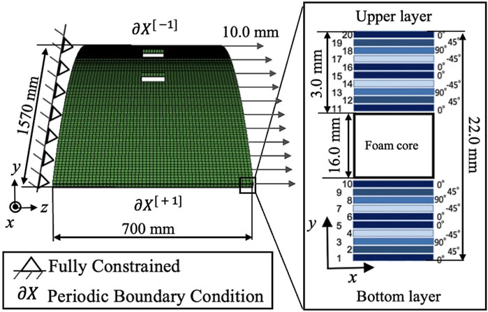
Figure 1. Analysis conditions of the perforated CFRP curved interstage structure. The model simulates a scaled-down curved panel subjected to tensile displacement along the $z$-direction, with periodic boundary conditions applied at both ends.

The dimensions of the curved panel are approximately $2000.0\text{\hspace{0.17em}mm}$ in radius, $1570.0\text{\hspace{0.17em}mm}$ in arc length, $700.0\text{\hspace{0.17em}mm}$ in vertical length, and $22.0\text{\hspace{0.17em}mm}$ in thickness. Square and rectangular holes are introduced at the center to simulate openings typically found in space launch vehicles: $100.0\text{\hspace{0.17em}mm}\times 100.0\text{\hspace{0.17em}mm}$ for square holes and $200.0\text{\hspace{0.17em}mm}\times 100.0\text{\hspace{0.17em}mm}$ for rectangular holes. The total thickness of the panel is $22.0\text{\hspace{0.17em}mm}$, consisting of a $3.0\text{\hspace{0.17em}mm}$–thick CFRP laminate on the top, a $16.0\text{\hspace{0.17em}mm}$–thick foam core in the middle, and another $3.0\text{\hspace{0.17em}mm}$–thick CFRP laminate at the bottom. This sandwich structure design ensures high stiffness while maintaining lightweight structure. The core material used for the CFRP-foam core sandwich structure is Rohacell 110WF, a polymethacrylimide (PMI) rigid foam manufactured by Evonik (Kobayashi, 2023). This material is widely used in aerospace applications owing to its high specific strength and stiffness, and stable mechanical properties even under cryogenic conditions.

The CFRP layers are composed of ten plies of unidirectional prepreg ($0.3\text{\hspace{0.17em}mm}$–thick each) laminated on both sides of the foam core (Shimazaki et al., 2015). The fiber orientations of the stacked unidirectional composites are $0°$, $45°$, $90°$, $-45°$, $0°$, $0°$, $-45°$, $90°$, $45°$, and $0°$. The $z$-axis in Figure 1 corresponds to the fiber direction of $0°$.

Defects are inserted away from the red box area, which is expected to be significantly affected by stress concentration around the hole under tensile loading. As shown in the white boxes in Figure 2, each defect measures $100.0\text{\hspace{0.17em}mm}\times 100.0\text{\hspace{0.17em}mm}\times 0.3\text{\hspace{0.17em}mm}$. Defects are implemented in the FEM model by modifying material properties to elements corresponding to the defect regions. Defects are inserted into the 18 internal plies excluding the top and bottom CFRP laminates, i.e., 1st and 20th layers and the foam core. The material properties of the CFRP, foam core, and defect regions are summarized in Table 1. To simulate interlaminar delamination, which is commonly performed in experiments by inserting Teflon sheets between prepregs layers (LÃpezâ et al., 2010), the material properties of Teflon sheets used in a previous study are referenced for the defect region (Kojima et al., 2022).

Figure 2

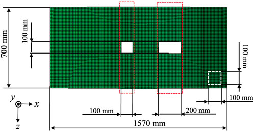
Figure 2. Representative example of defect insertion regions in the perforated CFRP curved interstage structure.

Table 1

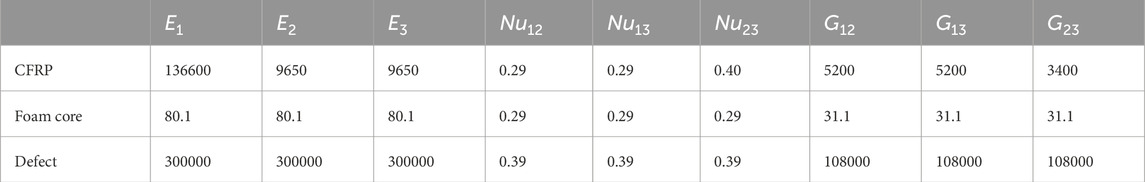
Table 1. Material properties of each region (Young’s modulus $E$ and shear modulus $G$ are in MPa.).

The mesh size is set to $12.5\text{\hspace{0.17em}mm}$. As boundary conditions, periodic boundary conditions are applied to both ends of the $z$-axis ($\partial X^{[+1]}$ and $\partial X^{[-1]}$). The left edge in the $x$-axis direction is fully constrained, whereas a uniform displacement boundary condition is applied at the right edge, with an imposed displacement of $10.0\text{\hspace{0.17em}mm}$ in the $z$-axis direction.

Under these conditions, FEM simulations are conducted to generate paired datasets consisting of the three-dimensional location of defects and the corresponding DSPSS on the curved panel. In total, one dataset without defects and 1,386 datasets with defects are prepared.

3.2 Proposed defect localization method

Figure 3 illustrates the proposed inverse defect localization framework. As shown in Figure 3a, for GNN training, we use only the DSPSS of the two outermost surface layers. As shown in Figure 3b, this method involves training a GNN using the normalized DSPSS obtained from FEM simulations to predict the three-dimensional location of defects.

Figure 3

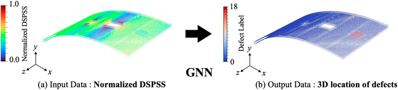
Figure 3. Proposed inverse defect localization framework using a GNN. (a) The input data consists of the normalized DSPSS, which is generated by FEM simulations. (b) GNN model predicts the three-dimensional location of defects by classifying each node with a discrete defect label.

To construct the training dataset, defects are inserted into the FEM model, and labels are assigned to the nodes corresponding to their locations, as shown in Figure 4. In this study, the 1st layer (bottommost) and 20th layer (topmost) of the CFRP structure are referred to as the bottom and upper surfaces respectively. Let $V$ be the set of nodes in the mesh graph, and let $y_i\in \{\mathrm{0,1},\dots ,18\}$ denote the class label assigned to node $v_i\in V$. The class label corresponds to the defect insertion layer index minus 1, as defined in Equation 12:

$y_i=\left\{\begin{array}{cc}{c}^{*}-1\hfill & \text{if node}{v}_i\text{lies\hspace{0.17em}on\hspace{0.17em}the\hspace{0.17em}upper\hspace{0.17em}surface\hspace{0.17em}of}\hfill \\ \hfill & \text{a\hspace{0.17em}defect inserted\hspace{0.17em}in\hspace{0.17em}layer}{c}^{*}\hfill \\ 0\hfill & \text{otherwise}\hfill \end{array}\right..(12)$

Figure 4

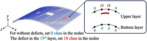
Figure 4. Ground truth labeling for each defect insertion layer. Each node is assigned a class index on the basis of its proximity to the defect: nodes within the defective layer are labeled from classes 1 to 18, corresponding to the 2nd to 19th plies. Nodes not adjacent to any defect are labeled class 0.

Using this labeling, we formulate the training objective as a 19-class node classification problem.

The group index for a given class $c$ is defined using the following grouping function, defined in Equation 13:

$\mathrm{g}\mathrm{r}\mathrm{o}\mathrm{u}\mathrm{p}\left(c\right)=\left\{\begin{array}{cc}0\hfill & \text{if} c+1\le 10\hfill \\ 1\hfill & \text{if} c+1\ge 11\hfill \end{array}\right..(13)$

GNN is then trained to solve a 19-class node classification problem on the basis of this input data and outputs the classification results. The training conditions of GNN are summarized in Table 2. Using this approach, we can construct a GNN capable of accurately estimating defect locations from DSPSS.

Table 2

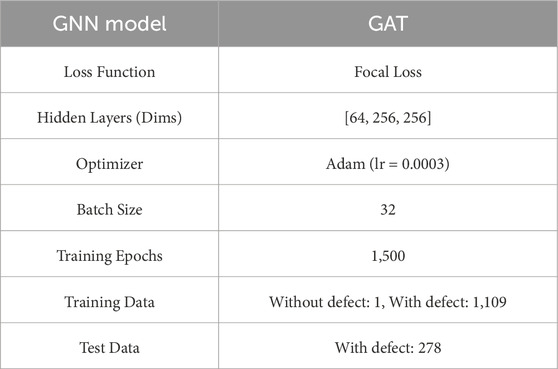
Table 2. Training conditions for GNN using surface DSPSS data.

3.3 Training conditions of GNN

Algorithm 1 outlines the training pipeline for a GNN model that predicts the three-dimensional location of defects from normalized DSPSS data. It covers data preprocessing, model architecture, distributed training with focal loss, test-time inference, and evaluation. In this study, GAT was constructed using three GATConv layers with hidden dimensions [64, 256, 256] and four attention heads. The attention mechanism is applied at each layer to effectively aggregate the input features. These aggregated features are then passed to a fully connected layer that performs final classification into 19 classes.

Algorithm 1

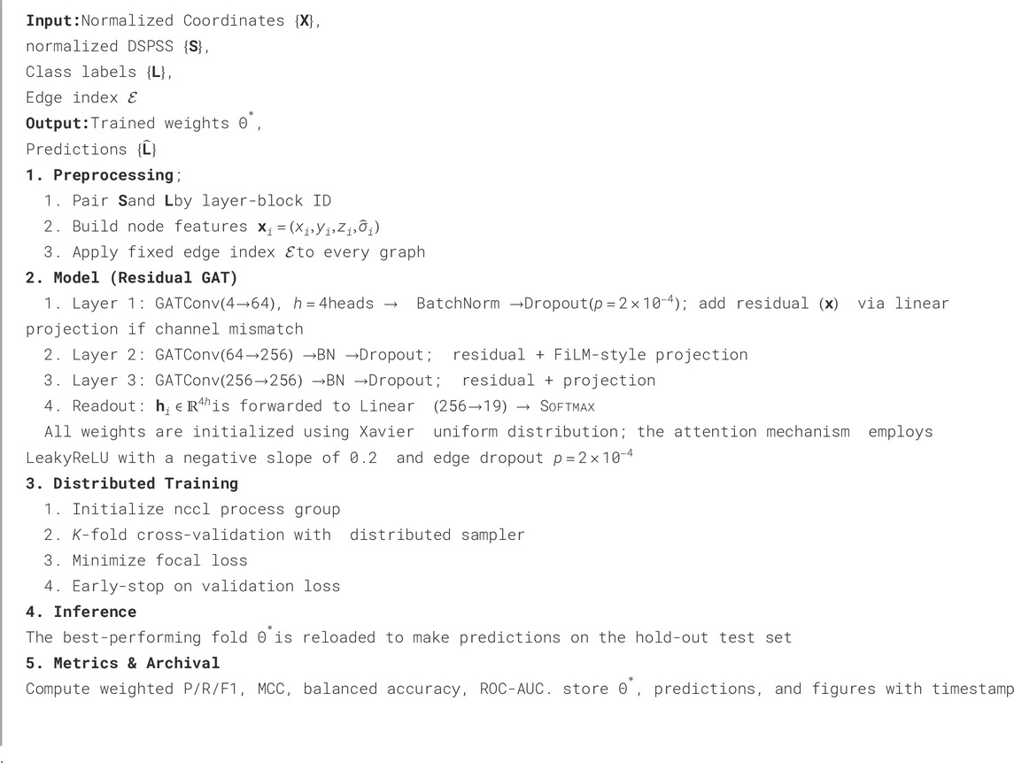
Algorithm 1. GNN Training.

To enhance training efficiency, distributed data parallelism was employed, allowing parallel computations across multiple GPUs. To assess the model's generalization capability, stratified five fold cross-validation was carried out. The full dataset was randomly divided into five equal-sized folds. One fold was used as the validation set, whereas the remaining four were used for training, so that every sample was evaluated exactly once. This random splitting procedure guarantees that the model's performance is assessed on diverse, nonoverlapping portions of the data, providing a reliable estimate of its capability to generalize.

During the training process, model evaluation was conducted at each epoch, and early stopping was applied if no performance improvement was observed, thus preventing overfitting. The best-performing model in each fold was saved and evaluated using the test dataset. Evaluation metrics included precision, recall, F1-score, and the confusion matrix, all of which were visualized to interpret performance. Finally, the model that achieved the lowest validation loss among all folds was selected as the final model for performance evaluation.

3.4 Loss function

In this study, we address an imbalanced classification problem in which the number of intact nodes significantly exceeds that of nodes containing defects. To handle this imbalance, focal loss (Lin et al., 2017), rather than conventional cross-entropy loss, is employed. Focal loss increases the loss contribution from misclassified examples whereas it decreases the loss contribution from well-classified ones, thereby encouraging the model to focus more on difficult-to-classify samples: in this case, the nodes contain defects. Since intact nodes dominate the dataset, their contribution to the overall loss is down-weighted accordingly.

The estimated probability $p_t$ is defined using $p$, as shown in Equation 14.

$p_t=\left\{\begin{array}{cc}p\hfill & \text{if} y=1\hfill \\ 1-p\hfill & \text{otherwise.}\hfill \end{array}\right.(14)$

Using this definition, we express the focal loss using Equation 15:

$\text{FL}\left(p_t\right)=-{\alpha }_t{\left(1-p_t\right)}^{\gamma }\log \left(p_t\right),(15)$

where $\gamma$ is the focusing parameter that controls the degree of down-weighting for well-classified examples and ${\alpha }_t$ is the weighting factor.

3.5 Evaluation method for prediction results

In this study, two evaluation metrics are used to quantitatively assess the accuracy of defect prediction: the planar defect location accuracy $R$ and the defect insertion layer prediction accuracy $P_{\text{gauss}}$. These metrics independently measure how accurately the model predicts the planar position and depth of each defect. The total defect prediction score (TDPS), defined as the average of these two metrics, serves as a unified metric for evaluating model performance on each defect case.

In addition, to evaluate the classification performance across the entire test dataset, in this study, we also adopt the macro-averaged F1-score. This metric is used to calculate the F1-score for each class individually and then takes the arithmetic mean across all classes, enabling fair evaluation even when the class distribution is imbalanced.

In the following subsections, we describe the definition of each metric in detail.

3.5.1 Prediction accuracy for each test data

The planar defect location accuracy $R$ is defined as the F1-score for the binary classification of whether each node contains a defect. The F1-score is the harmonic mean of precision and recall, as expressed in Equation 16.

$R=\text{F}1-\text{score}=\frac{2\times \text{Precision}\times \text{Recall}}{\text{Precision}+\text{Recall}}.(16)$

A higher $R$ value indicates higher accuracy of planar defect localization by the model.

To quantitatively evaluate the prediction accuracy of the defect insertion layer, we introduce $P_{\text{gauss}}$, a score based on a Gaussian-weighted function. This metric rewards predictions that are close to the correct class and penalizes those belonging to a different group. Specifically, the layers are divided into two groups: bottom layers (1st–10th) and upper layers (11th–20th). predictions falling into the incorrect group are assigned zero weight.

Let $N$ be the total number of nodes predicted as having a defect, $c_i$ the predicted class of the $i$-th node, $c*$ the ground truth class, and $\sigma$ the standard deviation for the Gaussian weight. Then, $P_{\text{gauss}}$ is defined in Equation 17 as

$P_{\text{gauss}}=\frac{1}{N}{\displaystyle \sum _{i=1}^N}{\delta }_{\text{group}}\left(c_i,c^{*}\right)\cdot \exp \left(-\frac{{\left(c_i-c^{*}\right)}^2}{2{\sigma }^2}\right),(17)$

where ${\delta }_{\text{group}}(c_i,c*)$ is a function that returns to 1 if the predicted and true classes belong to the same group and 0 otherwise, defined in Equation 18:

${\delta }_{\text{group}}\left(c_i,c^{*}\right)=\left\{\begin{array}{cc}1\hfill & \text{if} \mathrm{g}\mathrm{r}\mathrm{o}\mathrm{u}\mathrm{p}\left(c_i\right)=\mathrm{g}\mathrm{r}\mathrm{o}\mathrm{u}\mathrm{p}\left(c^{*}\right)\hfill \\ 0\hfill & \text{otherwise}\hfill \end{array}\right..(18)$

The layer grouping function is defined in Equation 19 as:

$\mathrm{g}\mathrm{r}\mathrm{o}\mathrm{u}\mathrm{p}\left(c\right)=\left\{\begin{array}{cc}0\hfill & \text{if} \left(c+1\right)\le 10\hfill \\ 1\hfill & \text{if} \left(c+1\right)\ge 11\hfill \end{array}\right..(19)$

This approach imposes strict penalties for misclassification between upper and lower layer groups, whereas allowing some tolerance for errors between neighboring layers within the same group. In this study, a standard deviation of $\sigma =2.0$ is used as the dispersion parameter for the Gaussian weight.

To quantify the overall defect prediction performance of the model, we define a composite metric called the TDPS, which is the average of the two metrics (see Equation 20).

$\text{TDPS}=\frac{R+P_{\text{gauss}}}{2}(20)$

A higher TDPS indicates that the model can accurately predict both the planar position and depth of the defect.

3.5.2 Overall model performance: macro-averaged F1-Score

To evaluate the classification performance equally across all classes, in this study, we adopt the macro-averaged F1-score as a quantitative metric. The macro-averaged F1-score is calculated as the arithmetic mean of the F1-scores computed individually for each class and is defined in Equation 21:

${\mathrm{F}\mathrm{1}}_{\text{macro}}=\frac{1}{C}{\displaystyle \sum _{i=1}^C}{\mathrm{F}\mathrm{1}}_i,(21)$

where $C$ denotes the number of classes, which equals 19 in this study, and ${\mathrm{F}\mathrm{1}}_i$ represents the F1-score for class $i$.

This metric treats all classes equally regardless of their frequency, making it particularly effective for imbalanced classification problems. By using this evaluation method, we can confirm that the model performs balanced learning across all classes without being biased toward the majority class, which corresponds to intact nodes.

4 Results and discussion

4.1 Stress distribution around defects

As shown in Figure 5a, presents the DSPSS in the physical coordinate system $(x,y,z)$, accurately representing the curvature of the actual structural surface.

Figure 5

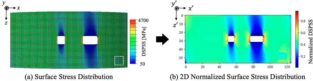
Figure 5. (a) Surface stress distribution with defect insertion. (b) Two-dimensional normalized surface stress distribution used for defect profiling.

Figure 5b projects the same data into a dedicated visualization space. By introducing a virtual coordinate system $(x^{\prime },y^{\prime },z^{\prime })$,the originally curved surface can be effectively unwrapped and flattened facilitating the inspection of spatial patterns.

Figure 6 presents the surface stress distribution obtained by FEM analysis along with vertical and horizontal stress profiles. The left panel shows the normalized DSPSS when a defect is inserted into the second layer $(45°)$. A significant stress drop is clearly visible around the defect region.

Figure 6

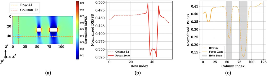
Figure 6. (a) Normalized DSPSS over the surface. Dashed lines indicate the vertical and horizontal cross sections through the defect center. (b) Stress profile along the vertical $z^{\prime }$–axis. Bold lines highlight the affected region around the defect. (c) Stress profile along the horizontal $x^{\prime }$–axis. The shaded area represents the hole region.

The central graph displays the vertical stress profile along the line passing through the center of the defect. A steep stress decrease is observed in the region corresponding to the defect. The right panel shows the horizontal stress profile across the defect center, indicating stress reduction effects caused by both the defect and the nearby hole.

Figure 7 shows the stress profiles in cases where a single defect is inserted into each of the 2nd–10th layers against the intact scenario. To visually distinguish the effects across layers, layers with the same ply angle are plotted using the same color: $45°$ layers (2nd, 9th) in blue, $-45°$ layers (3rd, 7th) in green, $90°$ layers (4th, 8th) in red, and $0°$ layers (5th, 6th, 10th) in purple. The plots reveal that the impact range and stress reduction patterns vary depending on the ply angle. For instance, in the $90°$ layers, a more abrupt and deeper stress drop is observed than in the other layers, suggesting that the relationship between the fiber orientation and the tensile direction significantly affects stress propagation. Conversely, layers oriented at $0°$ and $-45°$ tend to show more gradual stress gradients.

Figure 7

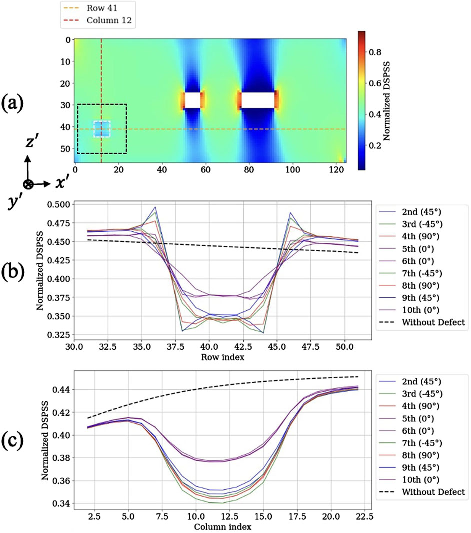
Figure 7. Comparison of DSPSS distributions and profiles for all defect-inserted inner layers. (a) Normalized DSPSS for a defect in the second layer. Dashed lines indicate vertical and horizontal reference lines. (b) Vertical stress profiles ($z^{\prime }$–axis) for all defect-inserted inner layers. (c) Horizontal stress profiles ($x^{\prime }$–axis) for all defect-inserted inner layers.

In the vertical stress profile shown in Figure 7b, each defect-inserted layer exhibits a distinct stress reduction around the defect center, hat clearly deviates from the intact stress distribution. This implies that the presence of defects can be quantitatively identified from surface stress information alone.

The vertical direction in Figure 7b corresponds to the $z^{\prime }$-axis, which aligns with the fiber direction of $0°$ in Figure 7a. Detailed characteristics according to the ply angle include the following.

$•$ 2nd and 9th layers $(45°)$: Owing to the angled fiber orientation, stress disperses more broadly, resulting in a wider area of stress reduction.

$•$ 3rd and 7th layers $(-45°)$: Similar distribution to $45°$ layers, but with minor left right asymmetry in the stress valley’s position and width.

$•$ 4th and 8th layers $(90°)$: As fibers are orthogonal to the out-of-plane direction, defect-induced stress shielding is more pronounced, with steeper and deeper stress drops.

$•$ 5th, 6th and 10th layers $(0°)$: Since the fiber direction aligns with the tensile direction, stress propagates more smoothly and the stress drop appears more gradual.

Similarly, in the horizontal stress profiles in Figure 7c, a significant reduction in stress is observed near the defect center, corresponding to the area affected by the defect. Compared with the healthy profile, all layers exhibit consistent stress drops, indicating that the model accurately captures the horizontal spatial positions of defects.

4.2 Evaluation of prediction results using R, P_gauss, and TDPS

Figure 8 shows the results of predicting the three-dimensional location of defects using the DSPSS obtained from FEM simulations as input. Figures 8a–d correspond to cases where defects were inserted into the 11th layer $(45°)$, 10th layer $(0°)$, 8th layer $(90°)$, and 2nd layer $(45°)$, respectively. Each case includes (i) the input data, (ii) ground truth labels, and (iii) outputs predicted by the model.

Figure 8

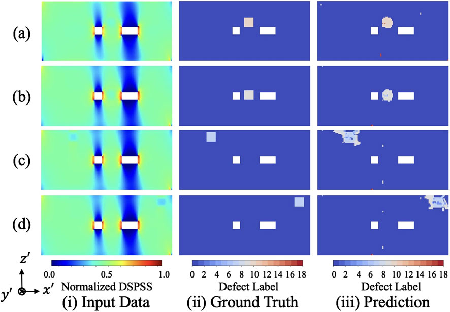
Figure 8. Comparison of (i) input data (normalized DSPSS), (ii) ground-truth labels, and (iii) model predictions for four representative cases, listed in descending order of the TDPS. (a) 11th layer ($45°$, highest TDPS); (b) 10th layer ($0°$, second-highest TDPS); (c) 8th layer ($90°$, second-lowest TDPS); (d) 2nd layer ($45°$, lowest TDPS).

Figure 8a represents the casewith the highest TDPS (0.92), which is the average of the planar defect location accuracy $R$ and the defect insertion layer prediction accuracy $P_{\text{gauss}}$. Figure 8b shows the case with second-highest TDPS (0.89), whereas Figures 8c,d correspond to the case with the second-lowest (0.50) and lowest (0.48) TDPS respectively.

Even in cases with low TDPS values, Both the planar position and the insertion layer are generally predicted with reasonable accuracy, as visually confirmed. This suggests that the proposed model successfully learns geometric features of internal defects in multilayered CFRP structures from DSPSS.

For all test data, the minimum value of the planar prediction metric $R$ was 0.55, indicating that the model can generally localize defects in the plane accurately. In many cases, the predicted defect region is slightly overestimated compared to the ground truth. On the other hand, the minimum layer prediction score $P_{\text{gauss}}$ was 0.38, indicating that the model is more sensitive to misclassification into neighboring layers or false detections in depth.

4.3 Prediction accuracy depending on defect insertion layer and planar position

Figure 10 shows the distribution of TDPS for each region (left, center, right), corresponding to the planar position where the defect was inserted. Here, TDPS is defined as the average of the planar defect prediction accuracy $R$ and the defect insertion layer prediction accuracy $P_{\text{gauss}}$. By plotting the TDPS for different regions, the figure illustrates how prediction performance varies with spatial location. The horizontal axis indicates each defect insertion layer along with its corresponding ply angle.

As shown in Figure 10a, the data points classified into the center region tend to exhibit higher TDPS than those classified into the left and right regions.

This tendency is primarily attributed to the characteristic of defects in the center region, which vary only in the $z^{\prime }$–axis direction and are located at a single position along the $x^{\prime }$–axis in the visualization space $(x^{\prime },y^{\prime },z^{\prime })$. In other words, since the center exhibits the narrowest spatial variation and the most consistent defect pattern, the model can more effectively learn representative features.

On the other hand, defects in the right and left regions are distributed widely in both the $x^{\prime }$– and $z^{\prime }$–directions, resulting in greater diversity and making the learning task relatively more difficult. Nevertheless, the performance difference in TDPS among these regions is modest, suggesting that the model can handle asymmetric fields with reasonable accuracy. In summary, prediction accuracy tends to increase in the order from the narrower search space: center, right, and left regions which are indicated by the yellow, red and blue respectively, in Figure 9.

Figure 9

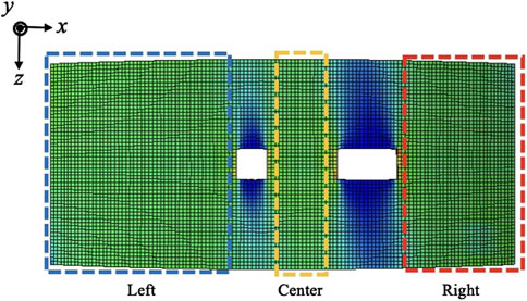
Figure 9. Planar segmentation of the specimen into three regions-left (blue), center (yellow), and right (red)-used to analyze the impact of defect location on prediction performance.

Regarding the planar position prediction metric $R$ shown in Figure 10b, the center region again demonstrates higher accuracy, whereas greater variation is observed in the left and right regions.

Figure 10

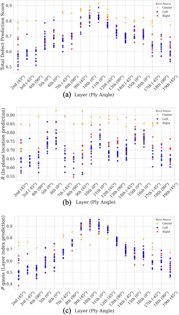
Figure 10. Comparison of prediction accuracy depending on defect insertion layer and planar position. (a) TDPS: the average of $R$ and $P_{\text{gauss}}$. (b) Planar prediction accuracy $R$. (c) Layer prediction accuracy $P_{\text{gauss}}$. The horizontal axis indicates the defect insertion layer and corresponding ply angle.

Regarding the defect insertion layer prediction metric $P_{\text{gauss}}$ shown in Figure 10c, the variation across depth is generally smaller, but the center region still achieves higher accuracy, indicating that the uniqueness of defects in the training data contributes to improved model performance.

Additionally, by examining the layer-wise trend, we observe that the TDPS are highest when defects are inserted into deeper layers (9th–12th), indicating more accurate defect recognition by the model. In contrast, when defects are inserted into the outermost layers (2nd–4th and 17th–19th), TDPS tends to decrease slightly.

4.4 Prediction accuracy depending defect insertion region

Figure 11 illustrates the comparison among the input data, ground truth, and model predictions for various defect locations within the same insertion layer (10th layer). The five subfigures correspond to distinct planar regions as defined in Figure 9. Despite differences in stress field distributions due to proximity to the holes and edges, the model successfully localizes the defect regions with high accuracy. Notably, the prediction performance remains consistent in both symmetric and asymmetric stress regions, demonstrating the robustness and generalization capability of the proposed GNN-based approach.

Figure 11

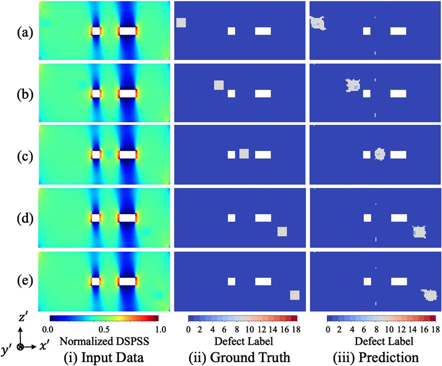
Figure 11. Comparison of (i) input data, (ii) ground truth, and (iii) predicted outputs for cases in which defects are inserted into the 10th layer at different planar regions defined in Figure 9. Specifically, (a,b) correspond to two different positions within the left region, (c) is from the center region, (d,e) correspond to the right region.

In all these cases, the TDPS remains high, with the highest being 0.89 and the lowest 0.82. This indicates that even when defects are located in regions with concentrated, peripheral, or nonuniform stress distributions, the proposed method maintains high prediction performance. These results suggest that the proposed approach is not sensitive to particular stress patterns and is robust across various stress distributions. Therefore, the model can stably detect internal defects by appropriately capturing subtle variations in stress fields caused by defects.

4.5 Prediction evaluation using confusion matrix

Figure 12 shows the confusion matrix for visualizing the prediction results for all nodes across 278 test data instances. The vertical axis represents the ground truth, whereas the horizontal axis represents the predicted classes. Each cell indicates the number of nodes classified into each category. For each ground truth class, precision and recall were calculated to derive the F1-score. The macro-averaged F1-score was obtained by averaging the F1-scores across all classes, resulting in 61%.

Figure 12

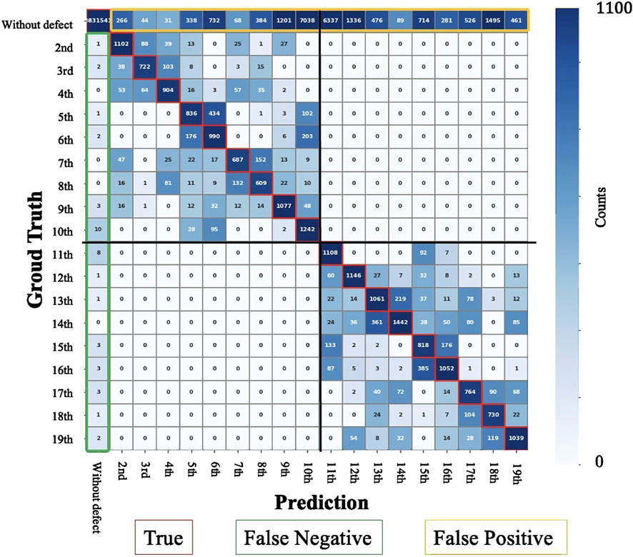
Figure 12. Confusion matrix for 19-class defect classification. Rows represent ground truth defect layers and columns denote predicted classes. Diagonal elements indicate correct predictions (True), whereas off-diagonal cells capture misclassifications. Green-line-enclosed cells represent false negatives (undetected defects), and yellow-line-enclosed cells indicate false positives (incorrect defect predictions in defect-free nodes). The results not only demonstrate high classification accuracy near the diagonal region but also reveal increased misclassification in adjacent layers.

In the green-line-enclosed area, the number of nodes misclassified as intact despite actually having defects is extremely low. This indicates that the proposed method rarely fails to detect defects and achieves high detection accuracy. The yellow-line-enclosed area indicates the number of nodes predicted as having defects when there were actually no defects, which correspond to false positives observed around defect edges in Figure 8.

The red-line-enclosed diagonal region represents the correctly classified nodes, and a large number of correct predictions can be observed. However, frequent misclassification into neighboring layers is also noticeable, which contributes to the reduction in macro-averaged F1-score. Misclassifications are most frequent in the deepest layers, specifically the 10th and 11th layers.

5 Conclusion

In this paper, we proposed a method of predicting the three-dimensional location of defects in perforated CFRP curved interstage structures, assuming Teflon sheets to represent artificial delamination defects within the prepreg layers. The method utilizes DSPSS obtained by FEM analysis as input. The following findings were confirmed:

$•$ Using GNN, we can accurately distinguish between defective and non-defective regions even for DSPSS not included in the training data.

$•$ The proposed model can localize both the planar position and defect insertion layer in models with hole geometries.

$•$ The macro-averaged F1-score achieved 61%, demonstrating high prediction accuracy even in the presence of inhomogeneous stress fields due to holes.

$•$ The average planar prediction accuracy $R$ was 72%, with a lowest value of 55%, indicating strong agreement between predicted and actual defect positions.

$•$ The depth prediction accuracy $P_{\text{gauss}}$, which incorporates tolerance to neighboring layer misclassification, yielded an average of 69% with a lowest value of 38%, confirming robust performance.

$•$ The average TDPS, defined as the mean of $R$ and $P_{\text{gauss}}$, was 70%, with a minimum of 48%, demonstrating that the model successfully predicts the three-dimensional location of defects with high accuracy.

Data availability statement

The raw data supporting the conclusions of this article will be made available by the authors, without undue reservation.

Author contributions

KN: Conceptualization, Data curation, Formal Analysis, Investigation, Methodology, Resources, Software, Validation, Visualization, Writing – original draft, Writing – review and editing. YK: Methodology, Supervision, Validation, Writing – review and editing. TS: Project administration, Supervision, Validation, Writing – review and editing. KK: Supervision, Validation, Writing – review and editing. MW: Supervision, Validation, Writing – review and editing. MM: Funding acquisition, Project administration, Resources, Supervision, Validation, Writing – review and editing.

Funding

The author(s) declare that no financial support was received for the research and/or publication of this article.

Conflict of interest

The authors declare that the research was conducted in the absence of any commercial or financial relationships that could be construed as a potential conflict of interest.

Generative AI statement

The author(s) declare that no Generative AI was used in the creation of this manuscript.

Any alternative text (alt text) provided alongside figures in this article has been generated by Frontiers with the support of artificial intelligence and reasonable efforts have been made to ensure accuracy, including review by the authors wherever possible. If you identify any issues, please contact us.

Publisher’s note

All claims expressed in this article are solely those of the authors and do not necessarily represent those of their affiliated organizations, or those of the publisher, the editors and the reviewers. Any product that may be evaluated in this article, or claim that may be made by its manufacturer, is not guaranteed or endorsed by the publisher.

References

Bagale, N., and Bhat, M. (2020). Evaluation of hygrothermal ageing in cfrp composite material using a non-destructive approach. J. Compos. Mater. 55 (9), 1309–1314. doi:10.1177/0021998320967054

CrossRef Full Text | Google Scholar

Byon, O., and Nishi, Y. (1998). Damage identification of cfrp laminated cantilever beam by using neural network. Key Eng. Mater. 141, 55–64. doi:10.4028/www.scientific.net/KEM.141-143.55

CrossRef Full Text | Google Scholar

Byon, Y. J., Lee, J. H., Kim, Y. Y., and Jang, H. S. (2008). Damage detection of cfrp composite structures using artificial neural networks. Compos. Struct. 84 (1), 65–74. doi:10.1016/j.compstruct.2007.08.012

CrossRef Full Text | Google Scholar

Caminero, M. Á., García-Moreno, Á. I., Rodríguez, G. P., and Chacón, J. M. (2019). Internal damage evaluation of composite structures using phased array ultrasonic technique: impact damage assessment in cfrp and 3d printed reinforced composites. Compos. Part B Eng. 165, 131–142. doi:10.1016/j.compositesb.2018.11.091

CrossRef Full Text | Google Scholar

Cawley, P., and Adams, R. (1987). “An automated coin-tap technique for the non-destructive testing of composite structures,” in Non-destructive testing of fibre reinforced plastics composites (Elsevier), 11–15.

CrossRef Full Text | Google Scholar

Chen, D., Tian, G., Woo, W. L., Pierce, S. G., Bryan, B. G., et al. (2012). Air-coupled ultrasonic infrared thermography for inspecting impact damages in cfrp. Chin. Opt. Lett. 10, 310401. doi:10.3788/COL201210.S10401

CrossRef Full Text | Google Scholar

Christensen, R. M. (2012). Mechanics of composite materials. Cour. Corp.

Google Scholar

Dilonardo, E., Nacucchi, M., Pascalis, F. D., Zarrelli, M., and Giannini, C. (2020). High resolution x-ray computed tomography: a versatile non-destructive tool to characterize cfrp-based aircraft composite elements. Compos. Sci. Technol. 192, 108093. doi:10.1016/j.compscitech.2020.108093

CrossRef Full Text | Google Scholar

Fang, Q., Ibarra-Castanedo, C., and Maldague, X. P. (2021). Automatic defects segmentation and identification by deep learning algorithm with pulsed thermography: synthetic and experimental data. Big Data Cognitive Comput. 5 (1), 9. doi:10.3390/bdcc5010009

CrossRef Full Text | Google Scholar

Gilmer, J., Schoenholz, S. S., Riley, P. F., Vinyals, O., and Dahl, G. E. (2017). “Neural message passing for quantum chemistry,” in Proceedings of the 34th international conference on machine learning (ICML), volume 70 of proceedings of machine learning research (Sydney, Australia: PMLR), 1263–1272.

Google Scholar

Hasebe, T., Higuchi, T., and Sato, T. (2020). Damage estimation of cfrp laminates using multi-task learning from surface strain distribution. Mech. Syst. Signal Process. 135, 106381. doi:10.1016/j.ymssp.2019.106381

CrossRef Full Text | Google Scholar

Hasebe, S., Higuchi, R., Yokozeki, T., and Takeda, S. I. (2023). Multi-task learning application for predicting impact damage-related information using surface profiles of cfrp laminates. Compos. Sci. Technol. 231, 109820. doi:10.1016/j.compscitech.2022.109820

CrossRef Full Text | Google Scholar

Hou, Y., Tie, Y., Li, C., Meng, L., Sapanathan, T., and Rachik, M. (2019). On the damage mechanism of high-speed ballast impact and compression after impact for cfrp laminates. Compos. Struct. 229, 111435. doi:10.1016/j.compstruct.2019.111435

CrossRef Full Text | Google Scholar

Ishikawa, M., Hatta, H., Habuka, Y., Jinnai, S., and Utsunomiya, S. (2012). Effect of anisotropic properties on defect detection by pulse phase thermography. Adv. Compos. Mater. 21 (1), 67–78. doi:10.1163/156855112x629513

CrossRef Full Text | Google Scholar

Ishikawa, M., Jinnai, S., Hatta, H., Utsunomiya, S., and Habuka, Y. (2013). “Reduction of phase noise to enhance detectable depth of defects in cfrps using pulse phase thermography,” in Proceedings of the 19th international conference on composite materials (ICCM-19) (Montreal, Canada), 8972–8979.

Google Scholar

Joas, S., Essig, W., Fröhlich, F. A., and Kreutzbruck, M. (2019). Cfrp pipe inspection by means of air-coupled ultrasound. AIP Conf. Proc. 2055, 120003. doi:10.1063/1.5084893

CrossRef Full Text | Google Scholar

Keo, S., Brachelet, F., Breabăn, F., and Defer, D. (2015). Defect detection in cfrp by infrared thermography with co2 laser excitation compared to conventional lock-in infrared thermography. Compos. Part B Eng. 69, 1–5. doi:10.1016/j.compositesb.2014.09.018

CrossRef Full Text | Google Scholar

Kidangan, R. T., Krishnamurthy, C. V., and Balasubramaniam, K. (2021). Identification of the fiber breakage orientation in carbon fiber reinforced polymer composites using induction thermography. NDT & E Int. 122, 102498. doi:10.1016/j.ndteint.2021.102498

CrossRef Full Text | Google Scholar

Kiefel, D., Stoessel, R., and Grosse, C. (2015). Quantitative impact characterization of aeronautical cfrp materials with non-destructive testing methods. AIP Conf. Proc. 1650, 591–598. doi:10.1063/1.4914658

CrossRef Full Text | Google Scholar

Kikukawa, H., and Ugai, T. (1997). Growth behavior of interlaminar delaminations at edge of circular hole of cfrp. J. Jpn. Soc. Aeronautical Space Sci. 45 (519), 380–386. doi:10.2322/jjsass1969.45.380

CrossRef Full Text | Google Scholar

Kobayashi, M. (2023). Damage evaluation of cfrp foam core sandwich structures and mechanical properties of adhesive joints under cryogenic conditions. Graduate School, The University of Tokyo.

Google Scholar

Kojima, Y., Hirayama, K., Endo, K., Hiraide, K., and Muramatsu, M. (2022). Inverse estimation method for internal defects based on surface stress of carbon-fiber-reinforced plastics using machine learning. Adv. Compos. Mater. 31 (6), 617–629. doi:10.1080/09243046.2022.2052786

CrossRef Full Text | Google Scholar

Kojima, Y., Hirayama, K., Harada, Y., and Muramatsu, M. (2024). Transfer-learning-aided defect prediction in simply shaped cfrp specimens based on stress distribution obtained from finite element analysis and infrared stress measurement. Compos. Part B Eng. 291, 111958. doi:10.1016/j.compositesb.2024.111958

CrossRef Full Text | Google Scholar

Li, H., Huo, Y., Cai, L., and Huang, Z. (2010). “Cfrp sandwiched facesheets inspected by pulsed thermography,” in Proceedings of SPIE - 5Th international symposium on advanced optical manufacturing and testing technologies: optoelectronic materials and devices for detector (China: Dalian), 7658 765855. doi:10.1117/12.865940

CrossRef Full Text | Google Scholar

Lãpezâ, A., MaimÃ, P., GonzÃlez, E. V., and RodrÃ-guez, J. (2010). Experimental study on delamination migration in composite laminates. Compos. Sci. Technol. 70 (6), 969–979. doi:10.1016/j.compscitech.2010.03.012

CrossRef Full Text | Google Scholar

Lee, S., Park, W., Lee, J. H., and Byun, J. (2006). “A study on non-contact ultrasonic technique for on-line inspection of cfrp,” in Proceedings of the Conference on Nondestructive Evaluation.

Google Scholar

Lin, T., Goyal, P., Girshick, R., He, K., and Dollár, P. (2017). “Focal loss for dense object detection,” in Proceedings of the IEEE international conference on computer vision (ICCV) (IEEE), 2980–2988.

Google Scholar

Maierhofer, C., Krankenhagen, R., Röllig, M., Rehmer, B., Gower, M., Baker, G., et al. (2018). Defect characterisation of tensile loaded cfrp and gfrp laminates used in energy applications by means of infrared thermography. Quantitative InfraRed Thermogr. J. 15 (1), 17–36. doi:10.1080/17686733.2017.1334312

CrossRef Full Text | Google Scholar

Mills, J. A., Hamilton, A. W., Gillespie, D. I., Andonovic, I., Michie, C., Burnham, K., et al. (2020). Identifying defects in aerospace composite sandwich panels using high-definition distributed optical fibre sensors. Sensors 20 (23), 6746. doi:10.3390/s20236746

PubMed Abstract | CrossRef Full Text | Google Scholar

Nasrin, N., Mohammadi, J., Ayatollahi, M. R., and Marzbanrad, E. (2023). Failure behavior of composite bolted joints: review. Appl. Mech. 3 (4), 834–859. doi:10.3390/appmech3040045

CrossRef Full Text | Google Scholar

Ning, F. D., Cong, W. L., Pei, Z. J., and Treadwell, C. (2016). Rotary ultrasonic machining of cfrp: a comparison with grinding. Ultrasonics 66, 125–132. doi:10.1016/j.ultras.2015.11.002

PubMed Abstract | CrossRef Full Text | Google Scholar

Pirinu, A., and Panella, F. (2021). Fatigue damage monitoring of cfrp elements by thermographic procedure under bending loads. Key Eng. Mater. 873, 47–52. doi:10.4028/www.scientific.net/kem.873.47

CrossRef Full Text | Google Scholar

Pohl, J. (2016). “Active thermographic testing of cfrp with ultrasonic and flash light activation,” in 19th World Conference on Non-Destructive Testing 2016, Köthen, Germany.

Google Scholar

Popow, V., and Gurka, M. (2020). Full factorial analysis of the accuracy of automated quantification of hidden defects in an anisotropic carbon fibre reinforced composite shell using pulse phase thermography. NDT & E Int. 116, 102359. doi:10.1016/j.ndteint.2020.102359

CrossRef Full Text | Google Scholar

Qiu, Y. M., Li, H., and Zhang, T. (2022). Thermographic stress analysis for principal stress evaluation in composite structures. Compos. Part B Eng. 239, 109913. doi:10.1016/j.compositesb.2022.109913

CrossRef Full Text | Google Scholar

Sakagami, T., Izumi, Y., Shiozawa, D., Fujimoto, T., Mizokami, Y., and Hanai, T. (2016). Nondestructive evaluation of fatigue cracks in steel bridges based on thermoelastic stress measurement. Procedia Struct. Integr. 2, 2132–2139. doi:10.1016/j.prostr.2016.06.267

CrossRef Full Text | Google Scholar

Scarponi, C., and Briotti, G. (2000). Ultrasonic technique for the evaluation of delaminations on cfrp, gfrp, kfrp composite materials. Compos. Part B Eng. 31 (3), 237–243. doi:10.1016/s1359-8368(99)00076-1

CrossRef Full Text | Google Scholar

Scarselli, F., Gori, M., Tsoi, A. C., Hagenbuchner, M., and Monfardini, G. (2009). The graph neural network model. IEEE Trans. Neural Netw. 20 (1), 61–80. doi:10.1109/tnn.2008.2005605

PubMed Abstract | CrossRef Full Text | Google Scholar

Shimazaki, Y., Tanaka, H., and Hara, H. (2015). “Application and issues of composite material structures in core rockets,” in Proceedings of the 31st Symposium on Space Structures and Materials, B05.

Google Scholar

Sobri, S. A., Whitehead, D., Mohamed, M., Mohamed, J. J., Mohamad Amini, M. H., Hermawan, A., et al. (2020). Augmentation of the delamination factor in drilling of carbon fibre-reinforced polymer composites (cfrp). Polymers 12 (11), 2461. doi:10.3390/polym12112461

PubMed Abstract | CrossRef Full Text | Google Scholar

Stoessel, R., Guenther, T., Dierig, T., Schladitz, K., Godehardt, M., Keßling, P., et al. (2011). μ-computed tomography for micro-structure characterization of carbon fiber reinforced plastic (cfrp). AIP Conf. Proc. 1335, 461–468. doi:10.1063/1.3591888

CrossRef Full Text | Google Scholar

Sultan, M. T. H., Worden, K., Pierce, S. G., Hickey, D., Staszewski, W. J., Dulieu-Barton, J. M., et al. (2011). On impact damage detection and quantification for cfrp laminates using structural response data only. Mech. Syst. Signal Process. 25 (8), 3135–3152. doi:10.1016/j.ymssp.2011.05.014

CrossRef Full Text | Google Scholar

Swiderski, W. (2019). Non-destructive testing of cfrp by laser excited thermography. Compos. Struct. 209, 710–714. doi:10.1016/j.compstruct.2018.11.013

CrossRef Full Text | Google Scholar

Torbali, M. E., Alhammad, M., Genest, M., Zhang, H., Zolotas, A., and Maldague, X. (2023). Enhanced defect identification by image fusion of infrared thermography and ultrasonic phased array inspection techniques. Thermosense Therm. Infrared Appl. XLV 12536 24. doi:10.1117/12.2659701

CrossRef Full Text | Google Scholar

Uchida, Y. (2021). Advanced infrared thermography techniques using visual imaging. Kobe, Japan: Kobe University.

Google Scholar

Uchida, T., Nakano, A., Sato, K., and Takami, K. (2021). Technologies for safe and resilient earthmoving operations: a systematic literature review. Automation Constr. 125, 103632. doi:10.1016/j.autcon.2021.103632

CrossRef Full Text | Google Scholar

Ura, K., Kajimura, S., Tanimae, I., and Maeda, T. (1998). Development of the h-iia rocket: improvements of composite interstage structures and propellant quantity measuring devices. Mitsubishi Heavy Ind. Tech. Rev. 5.

Google Scholar

VeliÄkoviÄ, P., Cucurull, G., Casanova, A., Romero, A., LiÃ, P., and Bengio, Y. (2018). “Graph attention networks,” in International conference on learning representations (Vancouver, Canada: ICLR).

Google Scholar

Wu, J.-Y., Sfarra, S., and Yao, Y. (2018). Sparse principal component thermography for structural health monitoring of composite structures. IFAC-PapersOnLine 51 (24), 855–860. doi:10.1016/j.ifacol.2018.09.675

CrossRef Full Text | Google Scholar

Yang, B., Huang, Y.-Y., and Cheng, L. (2013). Defect detection and evaluation of ultrasonic infrared thermography for aerospace cfrp composites. Infrared Phys. & Technol. 60, 166–173. doi:10.1016/j.infrared.2013.04.010

CrossRef Full Text | Google Scholar