AI-driven prediction of the impermeable boundary in karst rock mass for optimized anti-seepage curtain design

Introduction: Accurately determining the bottom boundary of anti-seepage curtains is critical for ensuring the integrity and performance of this key engineered composite structure in karst reservoirs. This study leverages artificial intelligence (AI) to address this materials design challenge.

Methods: We developed hybrid models by integrating a Genetic Algorithm (GA) with Backpropagation (BP), Support Vector Machine (SVM), and Extreme Learning Machine (ELM) algorithms. These models were trained and validated using a comprehensive dataset from the Dehou Reservoir, incorporating critical material and hydrogeological properties of the karst rock mass. A comparative analysis with Random Forest (RF), eXtreme Gradient Boosting (XGBoost), and Light Gradient Boosting Machine (LightGBM) was also conducted.

Results: The results demonstrated that GA optimization significantly enhanced predictive performance. The GA-BP model achieved superior accuracy (R² = 0.98, MSE = 7.58). Furthermore, from an engineering safety perspective, the GA-SVM model provided the most reliable recommendations, frequently yielding conservative depth estimates. The comparative analysis validated the competitive advantage of the proposed hybrid models over other benchmark algorithms.

Discussion: This research underscores the potential of AI-driven approaches for the performance prediction and rational design of engineered geomaterial systems. The findings offer a powerful tool for infrastructure projects in complex geological settings, balancing predictive accuracy with critical engineering safety considerations.

1 Introduction

Karstified rock masses, including carbonates, evaporites, and conglomerates with a carbonate matrix, are widely distributed around the world, covering more than 10% of the Earth’s surface (Milanović, 2018). Specifically, In China alone, karst landscapes occupy approximately 3.44 million km², accounting for 28.14% of the national territory (Zhao et al., 2018; Li et al., 2019; Fang et al., 2021). From a materials science perspective, these rock masses represent complex natural geomaterials characterized by intrinsic heterogeneity and anisotropy, primarily due to their multi-scale pore-fracture structures resulting from dissolution. The unique geological features of karst regions, such as caves, conduits, and fissures, which fundamentally alter the material’s permeability, present profound engineering challenges engineering challenges, including rocky desertification, ground instability, and water leakage (Xu and Huang, 1996; Milanović, 2003; Song et al., 2012; Feng et al., 2020). In water conservancy projects, the inadequate sealing performance of this natural geomaterial leads to reservoir leakage and tunnel inrushes, posing significant risks to project integrity, safety, and economy. Therefore, research into karstified rock masses holds profound significance for the prudent construction and seamless operation of water conservancy and hydropower projects.

One of the most pressing issues faced in karst regions pertaining to such engineering projects is the leakage. This phenomenon significantly affects the impoundment of reservoirs and hydropower stations, which presents substantial threats to project integrity (TVA-Tennessee Valley Authority, 1972; Yuan, 1991; Liu et al., 2021). To mitigate the negative influence of this issue, extensive research has been conducted, yielding various notable achievements. Currently, four primary methods are utilized to investigate the karst development in project sites: exploration (Lugeon, 1933), geophysical methods (Arandjelović, 1976; Zhao et al., 2021), numerical simulation (Li et al., 2021), and intelligent algorithms (Fu et al., 2022; Zhang et al., 2022; Xiao et al., 2024). Exploration is a precise yet costly traditional method that includes drilling and pitting. It reveals the actual conditions at the exploration site through in-situ sampling and testing. However, this method is often expensive. Conversely, geophysical methods can acquire continuous geological information and present data in 2D or even 3D formats (Al-Fares, 2011). Nonetheless, these methods typically require indirect interpretation of physical feedback results, which may not directly reflect geological conditions, and they often entail a degree of distortion. Numerical simulation offers the ability to model and predict seepage states (Fu et al., 2024), but such simulations are usually based on a series of assumptions. This leads to conditions that may differ from actual scenarios to some extent. Intelligent algorithms have emerged in recent years due to advancements in artificial intelligent technology (Chen et al., 2025). These algorithms can analyze and predict karst development based on statistical data and relevant materials without necessitating a thorough understanding of underlying geological principles. As geological data becomes increasingly abundant and algorithms improve, this approach has been widely utilized, resulting in numerous successful outcomes (Ge et al., 2023). However, the effectiveness of these algorithms is heavily dependent on data quality, and some researchers express concerns regarding their theoretical foundations, as the processes are predominantly mathematical rather than grounded in geological engineering theories. To address leakage issues resulting from karst development, targeted treatment measures are essential. The most common and critical measure is the construction of an anti-seepage grout curtain (Abkemeier and Stephenson, 2005; Riemer and Rer. Nat., 2015), which functions as a large-scale engineered composite material. This composite system is formed by injecting grout (a designed material) into the pore-fracture network of the natural karst geomaterial, effectively creating a new, low-permeability barrier. Beyond this underground approach, other alternatives include surface alternatives, and coupled surface and underground approaches. The underground alternative can be established through methods such as grout curtains (Abkemeier and Stephenson, 2005; Riemer and Rer. Nat., 2015), cavern plugs, and cutoff walls. This approach is generally effective and economical for disconnecting horizontal leakage channels. Nevertheless, it is less effective for vertical leakage channels. Conversely, surface alternatives (Šumarac, 2008) are designed to address vertical or surficial leakage but tend to be more costly. For many projects, a combination of treatments is necessary to achieve reliable anti-seepage results. Despite the availability of these methods, significant challenges persist. A primary challenge is reliably determining the bottom boundary of the impermeable curtain – a key parameter that defines the geometry, volume, and thus the cost and performance of this engineered composite material. Accurately predicting this boundary at a reasonable cost remains difficult.

To address this challenge, which is fundamentally a materials design optimization problem, this study employed a series of AI algorithms to predict and analyze the bottom boundary of the impermeable curtain using data derived from the boreholes at the Dehou Reservoir. A portion of the data was utilized to train the proposed algorithm for predictions, which was subsequently validated using the remaining data. We compiled and analyzed data from 217 boreholes along a 4,814 m long waterproof curtain and inputted it into the AI algorithms. This study analyzed the relationship between various impact factors and the bottom boundary of the waterproof curtain. The findings not only provide insights for predicting and delineating the bottom boundary of the waterproof curtain in karst regions but also serve as a valuable resource of data and algorithms for government policymakers and project engineers involved in related initiatives.

2 Site characterization

2.1 Project description

The Dehou Reservoir Project (DRP) is situated on the Dehou River, the right headstream of the Panlong River in Wenshan Prefecture, Yunnan Province (104°-104.5°E, 23.5°-24°N). It is one of the largest-scale water conservancy projects in karst regions. This project has the largest grouting curtain system in the world, with a length of 4.84 km and a grouting drift length of 30.7 × 10⁴ m, as illustrated in Figure 1.

Figure 1

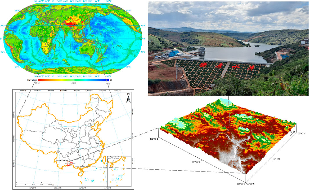
Figure 1. Study area.

The DRP mainly consists of a clay core rockfill dam with a height of 73.9 m and a crest length of 181.72 m, an anti-seepage curtain measuring 4,814 m within the dam site and reservoir area, a power station located behind the dam, and a water conveyance line. The DRP has a total capacity of 1.135 × 10⁸ m³ and a design irrigation area of 92,800 mu (approximately 6,186.67 ha). The dam includes one spillway and one flood discharge tunnel, which facilitate flood control. The dam was completed in March 2019. It started storing water in March 2020, and the water level reached normal levels in September 2021. After a water storage test, the anti-seepage performance met the predetermined objectives. By the end of 2022, the project successfully passed the completion acceptance. It has supplied a total of 284 million cubic meters of water, including over 100 million cubic meters for ecological purposes, and has generated more than 8 million kWh of electricity.

2.2 Geological settings

The dam is located within a distinctive V-shaped valley along the Dehou River, characterized by a meandering river channel and a riverbed width of approximately 200 m. The height of both banks is approximately 130 m. They exhibit a gentle slope upwards on one side and a steep slope downwards on the other side, with inclinations ranging from 10° to 70°. The lithology in the study area mainly consists of Quaternary loose deposits (Q), basalt from the upper Permian Emeishan group (P₂β), and siliceous rocks, siltstones, shales, and bauxites from the middle Permian Longtan group (P₂l). It also includes limestones, siliceous limestones, and dolomitic limestones from the lower Permian (P₁). Additionally, Permian Variscan basic intrusive rocks (βμ) and limestones from the upper (C₃) and middle series of the Carboniferous system (C₂), along with limestone, siliceous limestone, and siliceous rocks from the lower series of the Carboniferous system (C₁) were also identified (Figure 2). Notably, the carbonate rocks of the Carboniferous system (C₁, C₂, C₃) and Permian system (P₁) exhibit significant karstification, which poses a substantial risk of leakage in the reservoir.

Figure 2

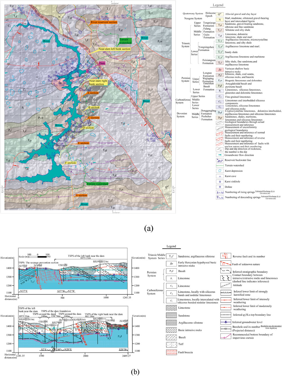
Figure 2. Geological and hydrogeological setting. (a) Engineering geological and hydrogeological map of the study area. (b) Engineering geological profile of the dam and its banks.

2.3 Hydrogeological overview

There are relatively impermeable strata, such as sandstone and mudstone between the Dehou River-Jiayi River block on the left bank of the reservoir area and the Mili River-Maguo River block on the right bank. Additionally, there is an underground watershed that is above the normal water storage level of the reservoir. Therefore, the potential for leakage from the reservoir to the low adjacent valleys of the Jiayi River and the Maguo River is relatively low. Underground watersheds were identified in sections C, D, and E of the Mili River-Panlong River block in the reservoir area (Figure 2). Leakage in these sections primarily occurs in the form of fractures and solution gaps, resulting in limited leakage volume. A certain amount of leakage is permissible, which allows for the optimization of anti-seepage treatment rather than its mandatory implementation. In section A of the Mili River, where non-carbonate rock is present, no leakage issues have been observed. Similarly, the underground watershed in section B of the Mili River is situated higher than the normal water level, thereby precluding any leakage concerns. However, significant karst leakage problems have been identified in section F of the Mili River-Panlong River block, as well as in the sections near the dam on both banks, including the dam foundation and surrounding areas. This leakage manifests in the form of karst pipelines and solution gaps, which necessitates the implementation of anti-seepage treatment. Therefore, the karst anti-seepage system for Dehou Reservoir consists of the dam foundation, seepage sections surrounding the dam site, sections adjacent to the dam on both the left and right banks, and section F of the Mili River reservoir area (Figure 2).

The bottom seepage control boundary was preliminarily determined based on karst development patterns and exploration data. The lower limit elevations of the strong karst zone in the dam foundation and the surrounding seepage sections, as well as near the left and right banks of the dam, ranged from 1,216 m to 1,240 m, 1,235 m to 1,265 m, and 1,200 m to 1,300 m. The lower limit elevation of the strong karst zone in section F of the Mili River reservoir area mostly ranged from 1,300 m to 1,350 m, and some local areas varied between 1,234 m and 1,280 m. There is a deep circulation zone characterized by intense karst development below a depth of 1,314 m. The lower limits of the strong karst zone in the dam foundation and the surrounding seepage sections, as well as near the left and right banks of the dam, were found to be 74–98 m lower than the riverbed elevation. Approximately 4 km downstream from the dam site, the Panlong River exposes T₂f sandstone and shale that extend about 2–2.5 km along the river. This restricts the potential of deeper karst development in the deep circulation zone adjacent to the dam site and reservoir banks.

Furthermore, the bottom seepage control boundary was finally established based on the following principles: 1) a depth of 10 m below the lower limit of the strong karst zone, and 2) a permeability rate (q) of ≤5Lu in the dam site and surrounding seepage sections, while section F of the Mili River reservoir is defined by a permeability rate (q) of ≤10Lu. Accordingly, the depth of curtain grouting was defined as follows: for the dam foundation and surrounding seepage sections, the depth ranges from 153.5 to 171.5 m; for the sections near the left bank of the dam, it ranges from 122.5 to 162.5 m; for the sections near the right bank of the dam, it is between 65.7 and 171.5 m; and for section F of the Mili River reservoir area, the depth predominantly ranges from 12.5 to 87.5 m, with some local areas ranging from 107.5 to 122.5 m.

3 Methodology

In this study, six algorithms were employed to predict the depth of the bottom boundary of the anti-seepage curtain, which serves as a critical factor for the waterproofing measures of the karst reservoir. Specifically, the GA algorithm was used to optimize the connection weights and threshold values of the BP, SVM, ELM algorithms to improve their stability and accuracy. The optimized algorithms were subsequently applied to predict the bottom boundary of the waterproofing curtain.

The calculation platform used for this research is specified as follows: 1) Operating system: Windows 10 Professional Edition (64bit); 2) Processor: 12th Gen Intel(R) Core (TM) i7-12700H@2.30 GHz; 3) Memory (RAM): 16.0 GB.

3.1 Data preparation

Data were collected from 217 pilot holes along the reservoir’s anti-seepage curtain. These data were systematically organized and analyzed to extract various potentially relevant factors, including the depth of the anti-seepage curtain’s bottom boundary, the groundwater level depth, the permeability rate, lithology, the lower limit depth of the strong karst zone, the depth of the top boundary of the relatively impermeable layer, faults, karst cavities, karst fractures, and zones of solution-corroded rock debris. Five typical factors were selected for training the algorithm: depth of the strong karst zone lower limit, depth of the top boundary of the relatively impermeable layer, groundwater level depth, permeability rate, and lithology (see Figure 3). The selection of these five features is grounded in the fundamental principles governing permeation flow in karstified rock masses. They holistically describe the key aspects of the permeation system: the thickness of permeation domain is defined by the depth of the strong karst zone lower limit and the depth of the top boundary of the relatively impermeable layer; the intrinsic transport properties of the rock mass within this domain are characterized by the permeability rate, a direct measure of secondary permeability; and lithology, which influences the susceptibility to karstification; the driving force for seepage is represented by the groundwater level depth, which reflects the hydraulic head conditions. This feature set provides a complete and physically meaningful parameterization of the system for predicting the required depth of the anti-seepage curtain.

Figure 3

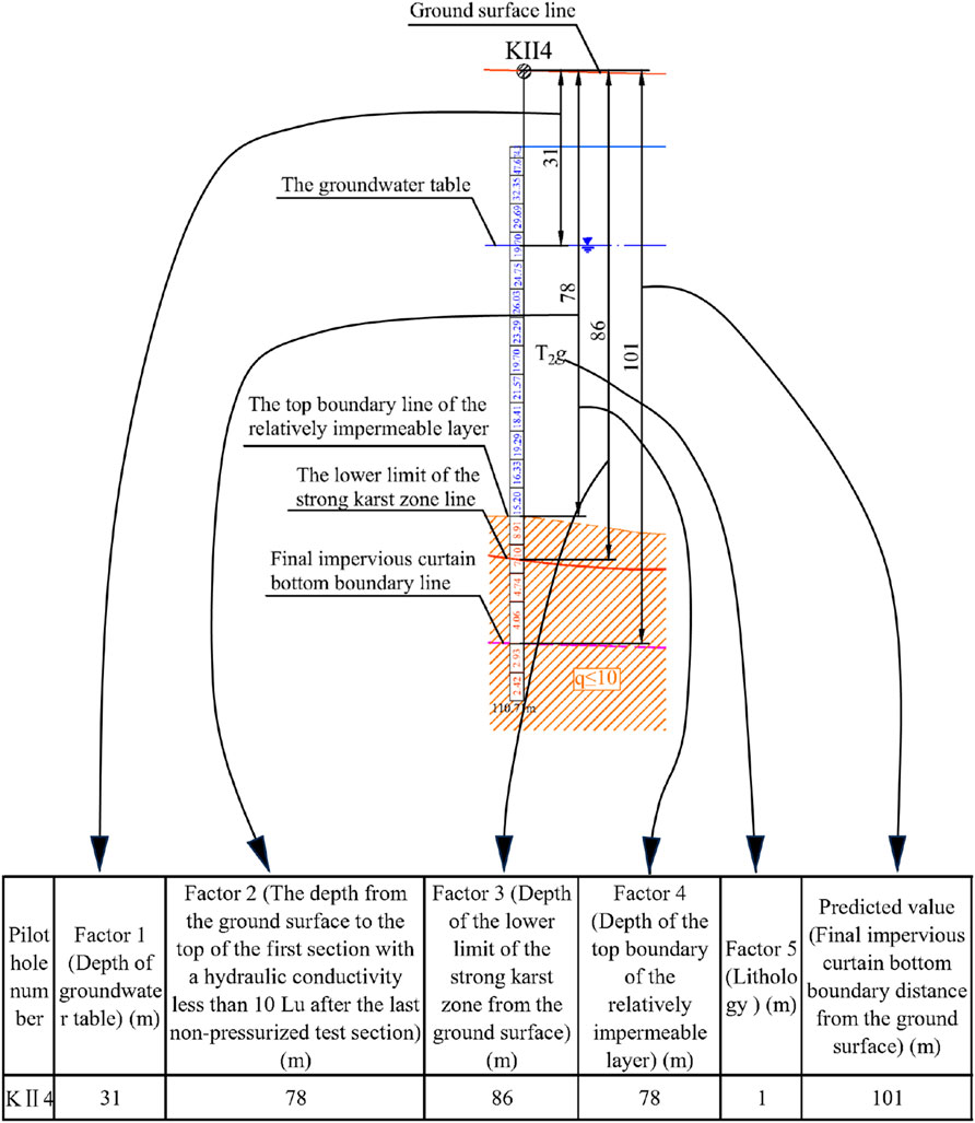
Figure 3. Data visualization graph.

Furthermore, the dataset was divided into a training set and a testing set in a ratio of 8:2. This split ensured that the models were trained and optimized solely on the training data, while the testing set, which the models never encountered during training, was strictly reserved for the final evaluation. The training set was utilized to train the algorithm for predicting the depth of the bottom boundary of the anti-seepage curtain, while the testing set was employed to evaluate the algorithm’s generalization ability. The results reported in Section 4 (e.g., R², MSE, and prediction errors) are all based on the predictions from this independent test set, thereby verifying the model’s practical utility and robustness.

3.2 Basic principles of the BP algorithm

The BP algorithm that serves as a cornerstone in the field of artificial neural networks (Rumelhart et al., 1986) facilitates the optimization of predictive and classification performance by iteratively adjusting the network’s weights and biases to minimize output error.

3.3 Basic principles of the SVM algorithm

The SVM is a supervised machine learning algorithm predominantly employed for classification and regression tasks (Vapnik, 1998). It classifies the data into distinct categories by identifying a hyperplane in a high-dimensional space using a kernel function. The “support vectors” are the data points that lie closest to the decision boundary or hyperplane. Therefore, this algorithm shows high efficiency and robustness.

3.4 Basic principles of the ELM algorithm

The ELM algorithm is one of the artificial neural network (ANN) algorithm (Huang et al., 2006) and is primarily utilized for supervised learning tasks. It is a single-layer feedforward network (SLFN), which means that information flows in a forward direction from the input nodes to the output nodes. In contrast to the traditional neural network training algorithms, The ELM algorithm randomly assigns the weights connecting the input layer to the hidden layer, which remain fixed during training. The weights connecting the hidden layer to the output layer are learned analytically in a single step. This unique approach results in rapid learning speed and high efficiency, particularly for large datasets.

3.5 Basic principles of the GA-BP algorithm

The GA-BP algorithm is a hybrid model that integrates the GA with the BP Algorithm. The BP algorithm, proposed by Rumelhart and McClelland (Rumelhart et al., 1988), is a gradient-based optimization algorithm aimed at minimizing the error between the predicted output of the network and the actual target output. However, it is prone to becoming trapped in local minima and exhibits slow convergence speed. The GA enhances this process by leveraging its global optimization capability, which is inspired by principles of natural selection and genetics (John, 1975). The procedure of the GA-BP algorithm is illustrated in Figure 4.

Figure 4

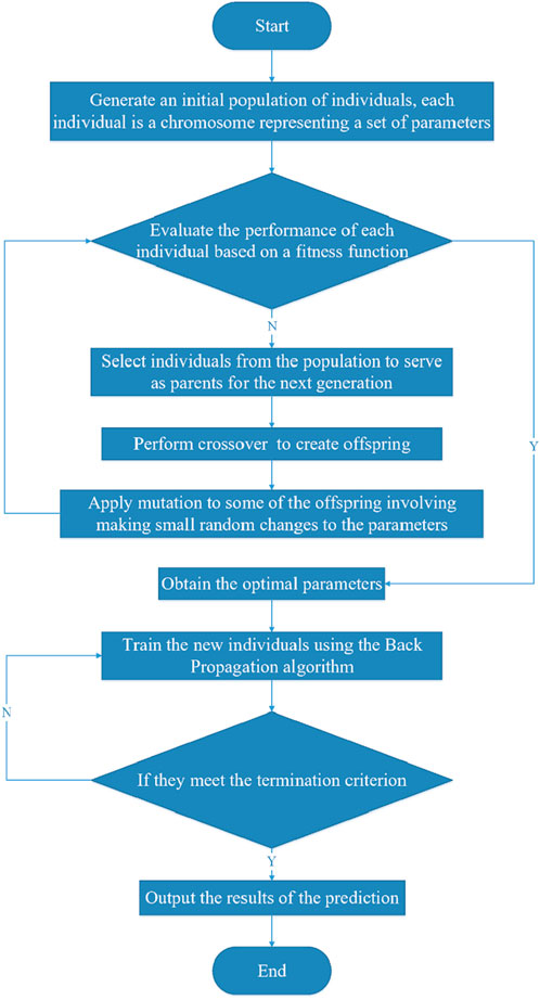
Figure 4. GA-BP algorithm flowchart.

3.6 Basic principles of the GA-ELM algorithm

The GA-ELM algorithm combines the optimization capabilities of the GA with the rapid learning mechanism of the ELM algorithm. The procedure of the GA-ELM algorithm is depicted in Figure 5.

Figure 5

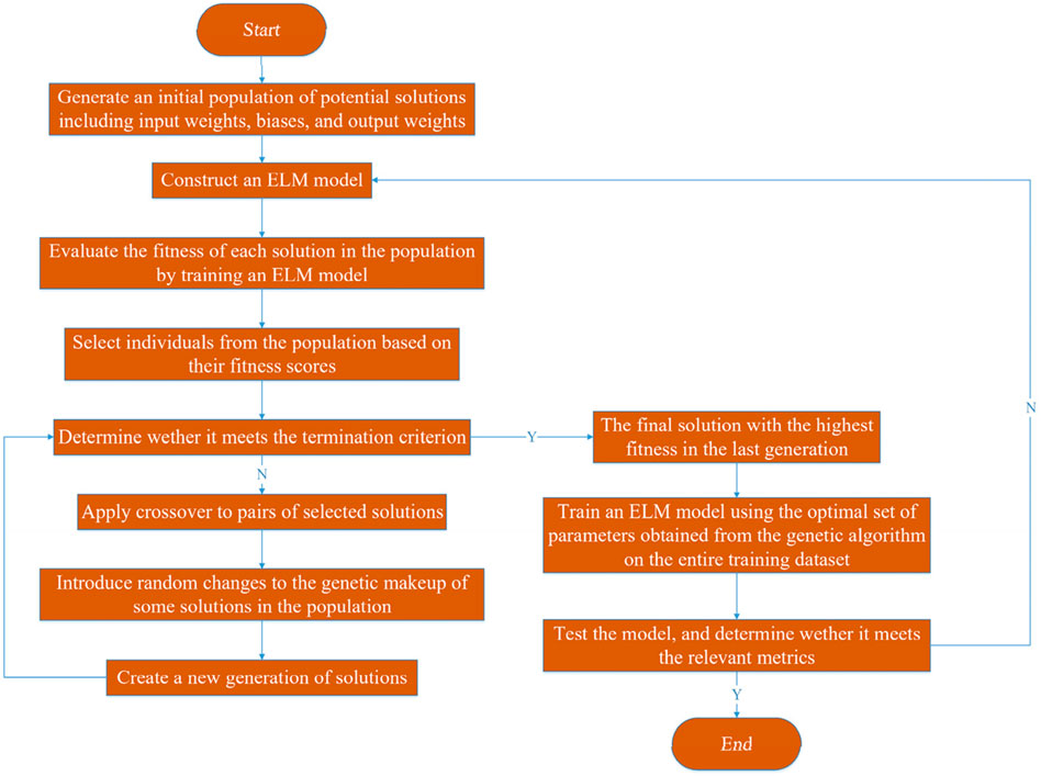
Figure 5. GA-ELM algorithm flowchart.

3.7 Basic principles of the GA-SVM algorithm

The GA-SVM is a hybrid algorithm that combines the optimization capabilities of the GA with the classification efficacy of the SVM algorithm. The procedure of the GA-SVM algorithm is illustrated in Figure 6.

Figure 6

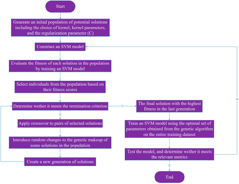
Figure 6. GA-SVM algorithm flowchart.

3.8 Principles of benchmark algorithms

To provide a comprehensive benchmark, three prevalent ensemble learning algorithms, Random Forest (RF), eXtreme Gradient Boosting (XGBoost), and Light Gradient Boosting Machine (LightGBM), were selected for comparison.

RF is an ensemble learning method that operates by constructing a multitude of decision trees at training time (Abdi et al., 2023). For regression tasks, the output is the mean prediction of the individual trees. RF introduces randomness by using bootstrapped datasets and random feature selection when splitting nodes, which enhances robustness and helps prevent overfitting.

XGBoost is an optimized distributed gradient boosting library designed to be highly efficient and scalable (Liang et al., 2020). It builds trees sequentially, where each new tree aims to correct the errors made by the previous ones. A key advantage is its incorporation of a regularization term in the loss function, which controls model complexity and further reduces overfitting.

LightGBM is a gradient boosting framework that uses tree-based learning algorithms (Li et al., 2023). It is designed for distributed computing and offers high efficiency with lower memory usage. Two innovative techniques it employs are Gradient-based One-Side Sampling (GOSS) and Exclusive Feature Bundling (EFB), which allow it to handle large-scale data much faster than many other algorithms.

4 Results

4.1 BP and GA-BP algorithms

The BP algorithm demonstrates a notable divergence from the desirable output values when compared to the GA-BP algorithm (see Figures 7b,d). For instance, at sample number 14, the predicted value by the BP algorithm was approximately 152.73, whereas the actual desirable output value was 184. This resulted in an error of 31.27, which represents the largest error among the BP results (see Figure 7a). This finding indicated a lower level of predictive accuracy. In contrast, the GA-BP algorithm yielded a predicted value of approximately 175.71 for the same sample number, with an error of 8.29. While it is the largest error in the GA-BP results, this algorithm still indicated a superior level of prediction (see Figures 7c,f). The prediction error plot in Figure 7f generally revealed that the GA-BP algorithm has a lower prediction error compared to the BP algorithm. This suggested that the GA-BP algorithm is more effective in minimizing the error. Additionally, both algorithms displayed a similar pattern concerning the relative variation in error magnitudes for their respective results across different samples.

Figure 7

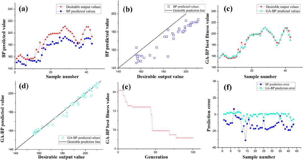
Figure 7. BP and GA-BP testing set prediction results: (a) BP testing set desirable output values and predicted values; (b) BP testing set predicted values and desirable prediction line; (c) GA-BP testing set desirable output values and predicted values; (d) GA-BP testing set predicted values and desirable prediction line; (e) GA-BP iteration graph; (f) BP and GA-BP prediction error.

As depicted in Figure 7e, the GA-BP algorithm’s fitness value decreased from 22 to 7.9, signifying an enhancement in the quality of the solutions. This pattern underscores the genetic algorithm’s proficiency in navigating the solution space. The lower prediction error of the GA-BP algorithm indicates a stronger potential for generalizing to new, unseen data sets. However, this enhanced accuracy of the GA-BP algorithm is accompanied by increased computational complexity due to the optimization processes inherent in the genetic algorithm. The trajectory of the fitness values of the GA-BP algorithm surpassed that of the BP algorithm, indicating a more effective optimization strategy. Notably, the GA-BP’s fitness value decreased to 7.9 after 100 iterations, while the BP algorithm’s fitness value remained constant (see Figure 7e).

Furthermore, since the predicted values represent the distance from the ground surface to the bottom boundary of the impermeable curtain, a predicted value exceeding the actual value results in a design scheme that is safer but less economical. Conversely, a predicted value that is less than the actual value leads to a more economical scheme but increases safety risks. Therefore, for engineering projects, a deviation greater than the actual value is generally more acceptable. The proportion of greater deviations in the BP algorithm was 2%, while that in the GA-BP algorithm was 63%. This comparison suggests that the GA-BP algorithm provides more reliable recommendations regarding the depth of the impermeable curtain bottom boundary when compared to the BP algorithm.

4.2 ELM and GA-ELM algorithms

The ELM algorithm exhibited a considerably greater divergence from the desired output values compared to the GA-ELM algorithm (see Figures 8b,d,f). For instance, at sample number 9, the predicted value generated by the ELM algorithm was approximately 261.23, whereas the desired output value was 168. This resulted in an error of 93.23, which is the largest in the ELM results (see Figure 8a). In contrast, the GA-BP algorithm aligns more closely with the desired values, and its largest error was approximately 29.38 (see Figures 8c,f). This indicates a similar optimization effect of the GA, which demonstrates better performance in terms of accuracy. The prediction error plot in Figure 8f revealed that the GA-ELM algorithm has a lower prediction error compared to the ELM algorithm. Notably, the error patterns of these two algorithms did not exhibit the same relative magnitude variations in their respective results for the corresponding samples as observed in the BP and GA-BP algorithms. This discrepancy can be attributed to the fact that the two algorithms used in this study did not employ entirely identical test sets. Nevertheless, it is evident that the optimization effectiveness of the GA remains significant across different test sets.

Figure 8

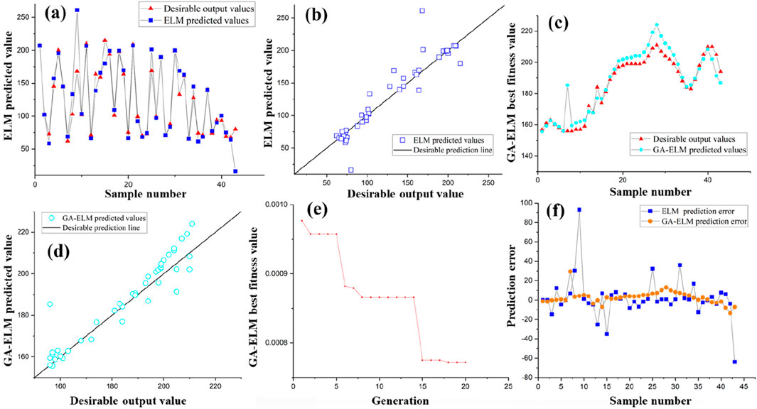
Figure 8. ELM and GA- ELM testing set prediction results: (a) ELM testing set desirable output values and predicted values; (b) ELM testing set predicted values and desirable prediction line; (c) GA- ELM testing set desirable output values and predicted values; (d) GA- ELM testing set predicted values and desirable prediction line; (e) GA- ELM iteration graph; (f) ELM and GA- ELM prediction error.

As shown in Figure 8e, the GA-ELM algorithm’s fitness value decreased from 9.8 × 10⁻⁴ to 7.7 × 10⁻⁴, signifying an enhancement in the quality of the solutions. This pattern underscores the genetic algorithm’s proficiency in exploring the solution space. Moreover, the GA-ELM algorithm demonstrates a stronger generalization capacity. The trajectory of the fitness values of the GA-ELM algorithm surpassed that of the BP algorithm, indicating a more effective optimization strategy. The GA-BP’s fitness value decreased to 7.7 × 10⁻⁴ after 20 iterations, while the ELM algorithm’s fitness value remained unchanged (see Figure 8e). Additionally, the GA-ELM algorithm converged more rapidly compared to the GA-BP algorithm.

Furthermore, the results indicated that the proportion of larger deviations in the ELM algorithm is 58%, which is much higher than that in the BP algorithm. In contrast, the GA-ELM algorithm exhibited an even higher proportion of 72%. This suggests that the GA- ELM algorithm provides more reliable recommendations regarding the depth of the impervious curtain bottom boundary when compared to the ELM algorithm.

4.3 SVM and GA-SVM algorithms

The SVM algorithm showed a more pronounced divergence from the desired output values than the GA-SVM algorithm (see Figures 9b,d,f). For instance, at sample number 15, the predicted value generated by the SVM algorithm was approximately 147.35, whereas the desired output value was 215. This resulted in an error of −67.65, which is the largest error observed in the SVM results (see Figure 9a). In contrast, the GA-BP algorithm aligned more closely with the desired values, and its largest error was approximately 9.82 (see Figures 9c,f). This reveals the similar optimization effect of the GA algorithm, which demonstrates superior performance in terms of accuracy. The prediction error plot in Figure 9f revealed that the GA-SVM algorithm has a lower prediction error compared to the SVM algorithm. Notably, the error patterns of these two algorithms did not exhibit the same relative magnitude variations in their respective results for the corresponding samples as observed in the ELM and GA- ELM algorithms. This can be attributed to the fact that the two algorithms used in this study do not utilize completely identical test sets. Thus, it can be reaffirmed that the test set influences the pattern of relative error variation. Nonetheless, it is evident that the optimization effectiveness of the GA remains significant across different test sets.

Figure 9

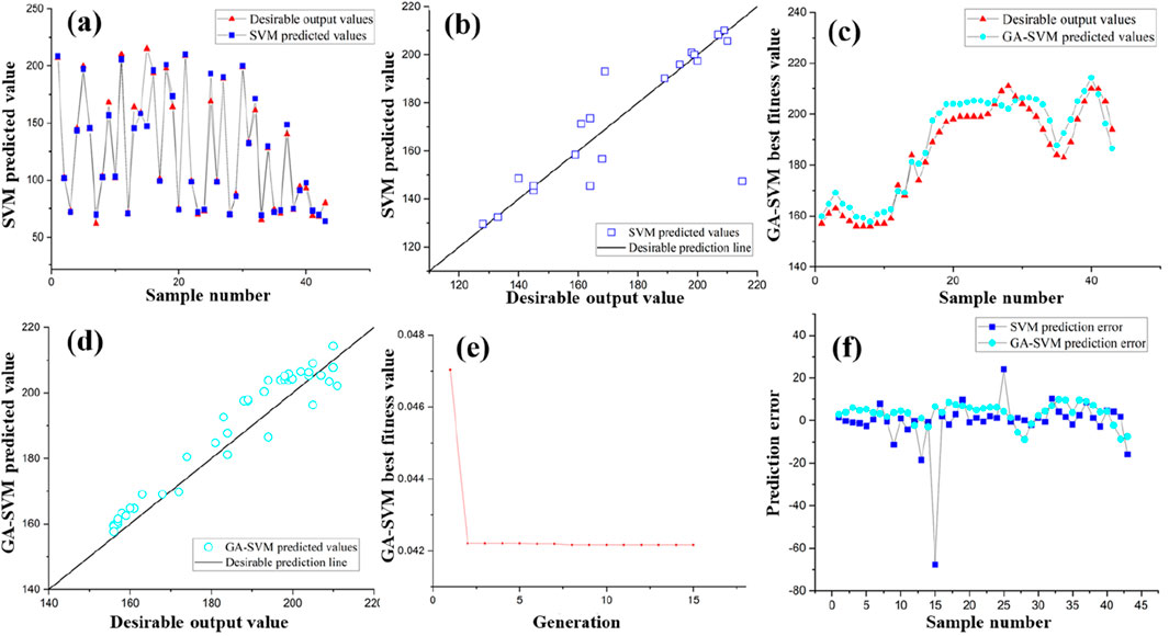
Figure 9. SVM and GA- SVM testing set prediction results: SVM and GA- SVM testing set prediction results: (a) SVM testing set desirable output values and predicted values; (b) BP testing set predicted values and desirable prediction line; (c) GA- SVM testing set desirable output values and predicted values; (d) GA- SVM testing set predicted values and desirable prediction line; (e) GA- SVM iteration graph; (f) SVM and GA- SVM prediction error.

As shown in Figure 9e, the GA-SVM algorithm’s fitness value decreased from 4.7 × 10⁻² to 4.2 × 10⁻², signifying an enhancement in the quality of the solutions. This further confirms the genetic algorithm’s proficiency in navigating the solution space and its stronger generalization capacity. The trajectory of the fitness values of the GA-SVM algorithm surpassed that of the BP algorithm, indicating a more effective optimization strategy. The GA-SVM’s fitness value decreased to 4.2 × 10⁻² after 15 iterations, while the SVM algorithm’s fitness value remained unchanged (see Figure 9e). Compared to the GA-BP and GA-ELM algorithms, the GA-SVM algorithm exhibited the fastest convergence.

Finally, the results indicated that the proportion of greater deviations in the SVM algorithm was 53%, which is substantially higher than that in the BP algorithm. In contrast, the GA-SVM algorithm exhibited an even higher proportion of 81%. Therefore, it can be concluded that the GA-SVM algorithm provides more reliable recommendations regarding the depth of the impervious curtain bottom boundary when compared to the SVM algorithm.

5 Discussions

To assess the accuracy of predictions obtained through various methods, we utilized the R² (see Equation 1) coefficient, Mean Squared Error (MSE) (see Equation 2), Root Mean Square Error (RMSE) (see Equation 3), and Residual Predictive Deviance (RPD) (see Equation 4) as metrics for precision evaluation. The R² coefficient measures the degree of closeness between the model’s predicted values and the actual observed values. Its value ranges from 0 to 1. An R² value closer to 1 indicates a better fit of the model to the data, which suggests that the differences between the model’s predicted values and the actual observed values are smaller. The MSE quantifies the difference between the model’s predicted values and the true values, where a smaller MSE indicates higher prediction accuracy of the model. The MSE amplifies larger errors through squared errors, which helps improve the prediction accuracy of the model. Similarly, a smaller RMSE value indicates higher prediction accuracy of the model. However, the RMSE, which is derived from the square root of these squared errors, is relatively less affected by outliers compared to MSE. The RPD assesses the relative magnitude of the dispersion of the model’s predicted values in relation to the actual observed values. A higher RPD value suggests that the dispersion of the predicted values is relatively smaller than that of the actual observed values, which generally indicates superior predictive performance of the model.

The R² coefficient can be calculated using the following formula:

$R^2=1-\frac{{\displaystyle {\sum }_{i=1}^n}{\left(y_i-{\widehat{y}}_i\right)}^2}{{\displaystyle {\sum }_{i=1}^n}{\left(y_i-\overline{y}\right)}^2}(1)$

where n is the number of samples, $y_i$ is the actual value of sample i, ${\widehat{y}}_i$ is the predicted value of sample i, $\overline{y}$ is the mean of the actual values.

The MSE can be calculated using the following formula:

$\text{MSE}=\frac{1}{n}{\displaystyle \sum _{i=1}^n}{\left(y_i-{\widehat{y}}_i\right)}^2(2)$

where the parameter definitions are consistent with those provided above.

The RMSE can be calculated using the following formula:

$\text{RMSE}=\sqrt{\frac{1}{n}{\displaystyle \sum _{i=1}^n}{\left(y_i-{\widehat{y}}_i\right)}^2}(3)$

where the parameter definitions are consistent with those provided above.

RPD is a metric employed to evaluate model performance by comparing the consistency between actual and predicted values. RPD can be calculated using the following formula:

$\text{RPD}=\frac{S_D\left(y_i\right)}{S_D\left(y_i-{\widehat{y}}_i\right)}(4)$

where $S_D\left(\right)$ is the standard deviation function.

5.1 Comparative analysis of BP, SVM and ELM algorithms

The results of the comparative analysis indicated that the BP algorithm exhibits a fluctuating prediction error. This observation suggests that while the BP algorithm can approximate the desired values, it may not consistently achieve high precision. This variability is further corroborated by the MSE value of 196.89 (see Table 1), which is notably higher than those of the SVM and ELM algorithms. The SVM algorithm, recognized for its efficacy in high-dimensional spaces, exhibited a desirable output value of 250 and a predicted value of 200. The prediction results showed a more stable performance compared to BP, which is reflected in a lower MSE of 147.98. The error chart for the SVM algorithm indicated a more consistent error margin, which is advantageous for applications requiring stable predictions. The high R² value of 0.94 suggested that the SVM algorithm captures a significant portion of the variance, and its fast training speed resulting from random initialization of hidden layer weights further contributes to its performance. In contrast, the ELM algorithm, despite its speed, recorded the lowest R² value of 0.87 among the three algorithms, indicating a less accurate model. The high MSE of 448.44 and the RMSE of 0.02 suggested that while the average error is low, the variance in ELM algorithm predictions is considerable.

Table 1

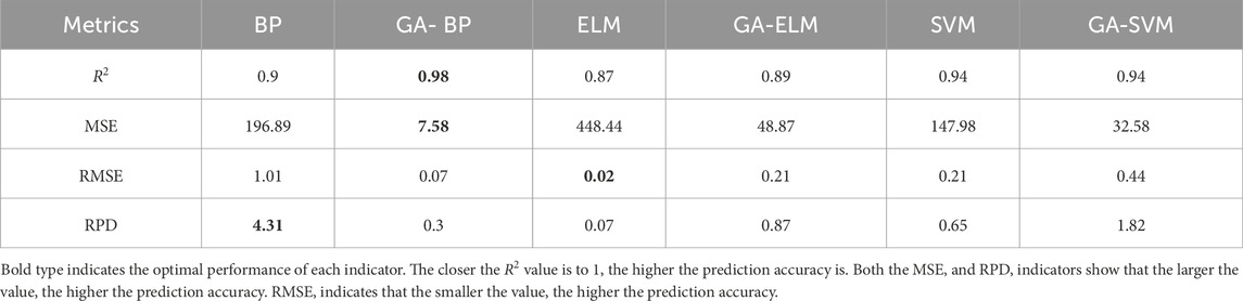
Table 1. The algorithm evaluation metrics.

The SVM algorithm outperforms both BP and ELM algorithms in terms of R² and MSE, indicating a superior fit to the data and lower average squared error. While the ELM algorithm is computationally efficient, it underperforms in predictive accuracy, as evidenced by the lower R² and higher MSE. Despite its simplicity and broad applicability, BP demonstrated greater variability in prediction errors, which may render it unsuitable for applications requiring high precision.

In summary, the SVM algorithm emerges as the optimal choice for tasks that require high accuracy and stability. Conversely, in scenarios where speed is paramount and a less accurate model is acceptable, the ELM algorithm may serve as a viable alternative. The BP algorithm, with its moderate performance, may be suitable for applications where model interpretability is an important consideration.

5.2 Comparative analysis of optimization with and without GA

The integration of the GA with traditional machine learning models has garnered considerable interest due to its potential to enhance model performance through effective optimization (Shi et al., 2025). The GA-optimized BP (GA-BP) model demonstrated a significant improvement over the standard BP model. Specifically, the R² value increased from 0.9 to 0.98 (see Table 1), indicating a more accurate representation of the variance in the data. The MSE dropped dramatically from 196.89 to 7.58, suggesting a substantial reduction in the average squared difference between the actual and predicted values. This optimization not only enhanced the predictive accuracy of the model but also improved its generalization capability, as evidenced by the reduced error metrics. Similarly, the GA-SVM model demonstrated considerable improvement over the standard SVM. While the R² value remained high at 0.94, the MSE was reduced from 147.98 to 32.58. This reduction indicates that GA optimization effectively fine-tuned the SVM model, resulting in more precise predictions. The RMSE decreased from 0.44 to 0.21, further emphasizing the enhanced accuracy of the model. The GA-ELM model experienced a notable improvement in performance. The R² value increased from 0.87 to 0.89—a modest but positive change. However, the most significant improvement was observed in the MSE, which dropped from 448.44 to 48.87. This substantial reduction in error indicates that GA optimization effectively refined the ELM model’s predictions, particularly in reducing the variance of the prediction errors.

Overall, the GA optimization process positively influenced all three algorithms, where GA-BP showed the most pronounced improvement in R² and MSE. This result suggests that GA optimization is particularly effective in enhancing the performance of BP. This effectiveness may be due to the algorithm’s dependency on weight adjustment, which aligns well with GA’s optimization capabilities. For tasks requiring high accuracy and robustness, the GA-BP algorithm may be the preferred choice. Conversely, for applications where a balance between accuracy and computational efficiency is paramount, the GA-SVM algorithm could be more suitable. In scenarios where rapid model deployment is necessary, the GA-ELM algorithm may offer an effective compromise between speed and accuracy.

5.3 The comprehensive analysis of the studied algorithms

The standard BP algorithm achieved an R² of 0.9, indicating that it explains 90% of the variance in the data. The MSE for this algorithm was 196.89, suggesting a relatively high prediction error. In contrast, the GA-BP algorithm demonstrated a substantial improvement in model accuracy, with an R² of 0.98 and an MSE of 7.58. This enhancement can be attributed to GA’s ability to fine-tune the weights of the BP model, leading to a more precise representation of the data. The SVM algorithm had an R² of 0.94 and an MSE of 147.98. However, the GA-SVM model achieved an MSE of 32.58, while maintaining the same R² value. This indicates that while GA optimization did not improve the model’s explanatory capability, it significantly reduced the prediction error. The ELM algorithm exhibited an R² of 0.87 and an MSE of 448.44. The GA-ELM model improved these metrics to 0.89 and 48.87, respectively. The increase in R² and the substantial reduction in MSE indicate that GA optimization enhanced the predictive accuracy of the ELM.

The RMSE values provide insights into the dispersion of the prediction errors. For the BP algorithm, the RMSE decreased from 1.01 to 0.07 with GA-BP (see Table 1). Similarly, the RMSE for the SVM reduced from 0.44 to 0.21 with GA-SVM, and for ELM, it reduced from 0.21 to 0.02 with GA-ELM. These reductions indicate that GA optimization not only improves accuracy but also reduces the variability of prediction errors across all models.

The iteration speed inferred from the fitness value plots indicated that the GA-BP and GA-SVM algorithms converge more rapidly than the GA-ELM algorithm. Specifically, the GA-BP and GA-SVM algorithms achieved optimal fitness values within 50 and 15 iterations, respectively, while the GA-ELM algorithm required 25 iterations. This suggests that the complexity of the optimization scenarios varies across models, with BP and SVM algorithms benefiting more rapidly from GA optimization.

The integration of GA with these algorithms has demonstrated an enhancement in their predictive capabilities. The GA-BP algorithm achieved the highest R² and the lowest MSE and RMSE, indicating superior accuracy and reduced error dispersion. While the GA-SVM algorithm did not show improvement in R², it demonstrated a significant reduction in both the MSE and RMSE, indicating improved reliability in predictions. Although the GA-ELM algorithm began from a lower baseline, it exhibited remarkable improvements. This makes it a viable option for scenarios requiring rapid model deployment.

From the perspective of guiding engineering design schemes, the GA-SVM algorithm can provide the most reliable recommendations regarding the depth of the impermeable curtain bottom boundary among the studied algorithms. In contrast, the BP algorithm presents the least favorable choice (see Table 2). The performance of the ELM and SVM algorithms is quite comparable, and this comparability aligns with that observed between the GA-ELM and GA-SVM algorithms. Furthermore, While the models presented in this study are data-driven, their predictive patterns and the identified feature importance are highly consistent with the fundamental geomechanical and hydrogeological principles that govern seepage in karst rock masses. Therefore, the model does not operate as an inscrutable “black box”; rather, it serves as a powerful non-linear regression tool that quantitatively captures and reinforces the long-established qualitative understanding of karst seepage control. This alignment between data-driven outcomes and physical principles significantly enhances the interpretability and credibility of our model for engineering applications.

Table 2

Table 2. The proportion of greater deviations in the results.

5.4 Benchmarking against prevalent machine learning models

To rigorously evaluate the performance of the proposed GA-optimized models, a comparative analysis was conducted against three widely-used machine learning algorithms: RF, XGBoost, and LightGBM. All models were trained and tested on the identical dataset (an 80/20 split) described in Section 3.1. The hyperparameters for all benchmark models were optimized via a grid search to ensure a fair comparison. The performance metrics on the independent test set are summarized in Table 3. The GA-BP model demonstrates superior predictive accuracy, achieving the highest R² and the lowest MSE and RMSE. This indicates that the hybrid GA-BP approach excels at modeling the complex underlying relationships in this specific regression task. Furthermore, for engineering applications where a conservative design is paramount, the GA-SVM model is particularly advantageous due to its highest RPD value and its tendency to over-predict the curtain depth, thereby reducing the risk of underseepage (He et al., 2025). While the benchmark models (especially XGBoost) show strong performance, this analysis confirms that our proposed GA-optimized models offer distinct and valuable performance characteristics.

Table 3

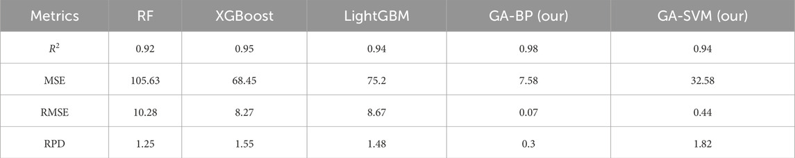
Table 3. Performance comparison with RF, XGBoost, and LightGBM.

5.5 Recommendations for future research

Based on the findings and limitations of this study, several promising avenues for future work are identified. Future research should prioritize the development of physics-informed neural networks (PINNs) or other mechanism-data hybrid models. By embedding governing equations (e.g., Darcy’s law, principles of flow in fractured media) into the architecture or loss function, predictions would be not only data-driven but also physically consistent, thereby enhancing interpretability and robustness in data-sparse scenarios (Li et al., 2024; Chen et al., 2021).

Furthermore, the current model is static and does not account for the dynamic evolution of karst systems. Future efforts should incorporate time-series data and long-term monitoring results to model the spatiotemporal evolution of seepage fields under the influence of reservoir operation and chemical dissolution.

Finally, to address the limited generalizability inherent in single-site studies, building large, multi-reservoir karst databases is essential. Exploring transfer learning techniques will be key to adapting models trained on large datasets to new karst regions with site-specific geological conditions, significantly boosting the engineering promotion value of the AI-aided design framework.

6 Conclusion

1. Traditional algorithms, including BP, ELM, and SVM, have demonstrated distinct advantages in predicting the bottom boundary for seepage control in karst reservoir regions. The SVM algorithm excelled in terms of accuracy and stability, while the ELM algorithm exhibited a notable advantage in speed. Although the BP algorithm demonstrated moderate performance, it offered commendable interpretability.

2. The GA demonstrated significant optimization effects in predicting the bottom boundary for seepage control in terms of predictive accuracy, error reduction, and convergence speed. The integration of the GA with these algorithms significantly improved the optimization process, resulting in a more precise and efficient predictive model. Notably, the optimization effect on the BP algorithm was particularly remarkable; however, its performance regarding the relative magnitude of error dispersion was less pronounced.

3. When choosing GA-BP, GA-SVM, and GA-ELM algorithms for predicting the bottom boundary for seepage control, it is essential to consider the specific requirements of the task, including accuracy, error dispersion, model training speed, and engineering safety. The GA-BP algorithm offered superior accuracy and reduced error dispersion, while the GA-SVM algorithm demonstrated improved prediction reliability. Although the GA-ELM algorithm began from a lower baseline, it showed notable improvements, which makes it a viable option for scenarios requiring rapid model deployment. The GA-SVM algorithm provided the most reliable recommendations regarding the depth of the impermeable curtain bottom boundary to enhance engineering safety.

Data availability statement

The original contributions presented in the study are included in the article/supplementary material, further inquiries can be directed to the corresponding author.

Author contributions

LZ: Conceptualization, Data curation, Formal Analysis, Investigation, Methodology, Resources, Validation, Visualization, Writing – original draft. ZT: Conceptualization, Formal Analysis, Funding acquisition, Project administration, Supervision, Validation, Writing – review and editing. RC: Conceptualization, Software, Supervision, Validation, Writing – review and editing. JW: Conceptualization, Funding acquisition, Investigation, Project administration, Supervision, Validation, Writing – review and editing. YZ: Funding acquisition, Investigation, Project administration, Supervision, Validation, Writing – review and editing. HT: Funding acquisition, Investigation, Project administration, Supervision, Writing – review and editing. BW: Data curation, Visualization, Writing – review and editing. CP: Conceptualization, Investigation, Supervision, Validation, Writing – review and editing. XH: Data curation, Formal Analysis, Investigation, Validation, Writing – review and editing. YZ: Methodology, Validation, Conceptualization, Visualization, Writing – review and editing.

Funding

The authors declare that financial support was received for the research and/or publication of this article. This work was financially supported by The Science and Technology Program Project of Yunnan Provincial Water Resources Department (Project Name: “Research on Anti-Seepage Measures for Reservoirs in Karst Areas”, Acceptance Certificate No.: 2023-001).

Acknowledgements

The authors thank Zhibo Wu, Hailin Ran, Jinyao Zhang, Jinxin Yang for the valuable suggestions, which significantly improved this paper.

Conflict of interest

Author LZ was employed by Yunnan Institute of Water and Hydropower Engineering Investigation and Design Co., Ltd.

Authors CP and XH were employed by CCC HongYu Water Conservancy Engineering Co., LTD.

The remaining authors declare that the research was conducted in the absence of any commercial or financial relationships that could be construed as a potential conflict of interest.

Generative AI statement

The authors declare that no Generative AI was used in the creation of this manuscript.

Any alternative text (alt text) provided alongside figures in this article has been generated by Frontiers with the support of artificial intelligence and reasonable efforts have been made to ensure accuracy, including review by the authors wherever possible. If you identify any issues, please contact us.

Publisher’s note

All claims expressed in this article are solely those of the authors and do not necessarily represent those of their affiliated organizations, or those of the publisher, the editors and the reviewers. Any product that may be evaluated in this article, or claim that may be made by its manufacturer, is not guaranteed or endorsed by the publisher.

References

Abdi, Y., Momeni, E., and Armaghani, D. J. (2023). Elastic modulus estimation of weak rock samples using random forest technique. Bull. Eng. Geol. Environ. 82 (5), 176. doi:10.1007/s10064-023-03154-y

CrossRef Full Text | Google Scholar

Abkemeier, T. J., and Stephenson, R. W. (2005). Remediation of a sinkhole induced by quarrying. ASCE Geotech. Spec. Publ. 122, 605–614. doi:10.1061/40698(2003)55

CrossRef Full Text | Google Scholar

Al-Fares, W. (2011). Contribution of the geophysical methods in characterizing the water leakage in afamia B dam, Syria. J. Appl. Geophys. 75, 464–471. doi:10.1016/j.jappgeo.2011.07.014

CrossRef Full Text | Google Scholar

Arandjelović (1976). Geophysics in the Karst. Special Edn. 17. Geozavod: Geophysical Institute.

Google Scholar

Chen, J., Yang, T., Zhang, D., Huang, H., and Yu, T. (2021). Deep learning based classification of rock structure of tunnel face. Geosci. Front. 12 (1), 395–404. doi:10.1016/j.gsf.2020.04.003

CrossRef Full Text | Google Scholar

Chen, H., Wang, K., Zhao, M., Chen, Y., and He, Y. (2025). A CNN-LSTM-Attention based seepage pressure prediction method for Earth and rock dams. Sci. Rep. 15 (1), 12960. doi:10.1038/s41598-025-96936-1

PubMed Abstract | CrossRef Full Text | Google Scholar

Fang, Q., Du, J.-M., Li, J.-Y., Zhang, D.-L., and Cao, L.-Q. (2021). Settlement characteristics of large-diameter shield excavation below existing subway in close vicinity. J. Central South Univ. 28 (3), 882–897. doi:10.1007/s11771-021-4628-7

CrossRef Full Text | Google Scholar

Feng, S., Zhao, Y., Wang, Y., Wang, S., and Cao, R. (2020). A comprehensive approach to karst identification and groutability evaluation – a case study of the dehou reservoir, SW China. Eng. Geol. 269 (May), 105529. doi:10.1016/j.enggeo.2020.105529

CrossRef Full Text | Google Scholar

Fu, H.-Y., Zhao, Y.-Y., Ding, H.-J., Rao, Y.-K., Yang, T., and Zhou, M.-Z. (2022). A novel intelligent displacement prediction model of Karst tunnels. Sci. Rep. 12 (1), 16983. doi:10.1038/s41598-022-21333-x

PubMed Abstract | CrossRef Full Text | Google Scholar

Fu, B., Pei, J. J., and Ji, H. (2024). Numerical simulation of three-dimensional seepage field in a tailing pond under multiple operating conditions. Sci. Rep. 14 (1), 28027. doi:10.1038/s41598-024-75988-9

PubMed Abstract | CrossRef Full Text | Google Scholar

Ge, Q., Sun, H., Liu, Z., and Xu, W. (2023). A data-driven intelligent model for landslide displacement prediction. Geol. J. 58 (6), 2211–2230. doi:10.1002/gj.4675

CrossRef Full Text | Google Scholar

He, P., Chen, Y., Feng, J., Wang, G., and Jiang, Y. (2025). An approach to rapidly evaluating rock mass quality in underground engineering based on multi-source heterogeneous data. Rock Mech. Rock Eng. 58, 1295–1325. doi:10.1007/s00603-024-04185-x

CrossRef Full Text | Google Scholar

Huang, G.-B., Zhu, Q.-Y., and Siew, C.-K. (2006). Extreme learning machine: theory and applications. Neurocomputing 70 (1–3), 489–501. doi:10.1016/j.neucom.2005.12.126

CrossRef Full Text | Google Scholar

John, H. H. (1975). Adaptation in natural and artificial systems.

Google Scholar

Li, P., Wang, F., Fan, L., Wang, H., and Ma, G. (2019). Analytical scrutiny of loosening pressure on deep twin-tunnels in rock formations. Tunn. Undergr. Space Technol. 83 (January), 373–380. doi:10.1016/j.tust.2018.10.007

CrossRef Full Text | Google Scholar

Li, S., Wang, X., Xu, Z., Mao, D., and Pan, D. (2021). Numerical investigation of hydraulic tomography for mapping karst conduits and its connectivity. Eng. Geol. 281 (February), 105967. doi:10.1016/j.enggeo.2020.105967

CrossRef Full Text | Google Scholar

Li, L., Liu, Z., Shen, J., Wang, F., Qi, W., and Jeon, S. (2023). A LightGBM-Based strategy to predict tunnel rockmass class from TBM construction data for building control. Adv. Eng. Inf. 58 (58), 102130. doi:10.1016/j.aei.2023.102130

CrossRef Full Text | Google Scholar

Li, X., Chen, Z., Tang, L., Chen, C., Ling, J., Tao, Li., et al. (2024). Predicting rock mass rating ahead of the tunnel face with bayesian estimation. Front. Earth Sci. 12, 1333117. doi:10.3389/feart.2024.1333117

CrossRef Full Text | Google Scholar

Liang, W., Luo, S., Zhao, G., and Wu, H. (2020). Predicting hard rock pillar stability using GBDT, XGBoost, and LightGBM algorithms. Mathematics 8 (5), 765. doi:10.3390/math8050765

CrossRef Full Text | Google Scholar

Liu, B., Wang, C., Liu, Z., Xu, Z., Nie, L., Pang, Y., et al. (2021). Cascade surface and borehole geophysical investigation for water leakage: a case study of the Dehou Reservoir, China. Eng. Geol. 294, 106364. doi:10.1016/j.enggeo.2021.106364

CrossRef Full Text | Google Scholar

Lugeon (1933). Barages at geologie. Paris: Dunod.

Google Scholar

Milanović, P. (2003). Prevention and remediation in Karst engineering. Sink. Eng. Environ. Impacts Karst, 3–30. doi:10.1061/40698(2003)1

CrossRef Full Text | Google Scholar

Milanović, P. (2018). Engineering karstology of dams and reservoirs. Belgrade: CRC Press.

CrossRef Full Text | Google Scholar

Riemer, W.Rer. Nat. (2015). “Investigation and treatment of problematic foundations for storage dams: some experience.” Springer International Publishing 6. doi:10.1007/978-3-319-09060-3_138

CrossRef Full Text | Google Scholar

Rumelhart, D. E., Hinton, G. E., and Williams, R. J. (1986). Learning representationsby back-propagating errors. Nature 323, 533–536. doi:10.1038/323533a0

CrossRef Full Text | Google Scholar

Rumelhart, D. E., Hinton, G. E., and Williams, R. J. (1988). “Learning internal representations by error propagation,” in Readings in cognitive science (Elsevier). doi:10.1016/B978-1-4832-1446-7.50035-2

CrossRef Full Text | Google Scholar

Shi, F., Liao, H., Wang, S., Omar, A., and Qu, F. (2025). Optimization of drilling rate based on genetic algorithms and machine learning models. Geoenergy Sci. Eng. 247, 213747. doi:10.1016/j.geoen.2025.213747

CrossRef Full Text | Google Scholar

Song, K.-I., Cho, G.-C., and Chang, S.-B. (2012). Identification, remediation, and analysis of karst sinkholes in the longest railroad tunnel in South Korea. Eng. Geol. 135–136 (May), 92–105. doi:10.1016/j.enggeo.2012.02.018

PubMed Abstract | CrossRef Full Text | Google Scholar

Šumarac, V. (2008). “Application of geomembrane to prevent water seepage from Ourkis Reservoir, Algeria,” in Paper presented at first congress of Serbian commitee for large dams, Bajna Bašta, Serbia.

Google Scholar

“TVA-Tenneesse Valley Authority(1972). TVA-tenneesse valley authority technical report, 16.

Google Scholar

Vapnik, V. (1998). Statistical learning theory. Wiley.

Google Scholar

Xiao, H., Cao, R., Wang, Y., Zhao, Y., and Sun, Y. (2024). Research on preprocessing methods for monitoring drilling data. J. Hydraulic Eng. 55 (11), 1379–1390. doi:10.13243/j.cnki.slxb.20230816

CrossRef Full Text | Google Scholar

Xu, J., and Huang, S. (1996). Mechanism of burst mud and Spring water of the dayaoshan tunnel. J. Railw. Eng. Soc. (02), 83–89. (In Chinese).

Google Scholar

Yuan, D. (1991). Karst of China. Beijing: Geological publishing house.

Google Scholar

Zhang, Y., Tian, Y., Ying, L., Wang, D., Tao, J., Yang, Y., et al. (2022). Machine learning algorithm for estimating karst rocky desertification in a peak-cluster depression Basin in southwest Guangxi, China. Sci. Rep. 12 (1), 19121. doi:10.1038/s41598-022-21684-5

PubMed Abstract | CrossRef Full Text | Google Scholar

Zhao, L., Zhang, S., Deng, M., and Wang, X. (2021). Statistical analysis and comparative study of multi-scale 2D and 3D shape features for unbound granular geomaterials. Transp. Geotech. 26, 100377. doi:10.1016/j.trgeo.2020.100377

CrossRef Full Text | Google Scholar

Zhao, Y., Wang, F., Li, C., Cao, Y., and Tian, H. (2018). Study of the corrosion characteristics of tunnel fissures in a karst area in southwest China. Geofluids 2018 (July), 1–19. doi:10.1155/2018/6234932

CrossRef Full Text | Google Scholar