Classical signature of quantum annealing

A pair of recent articles [1, 2] concluded that the D-Wave One machine actually operates in the quantum regime, rather than performing some classical evolution. Here we give a classical model that leads to the same behaviors used in those works to infer quantum effects. Thus, the evidence presented does not demonstrate the presence of quantum effects.

1. Introduction

Adiabatic quantum computation [3] has been shown to be equivalent to the usual circuit model [4]. This is only known to hold for ideal systems without noise. While there are effective techniques for fault-tolerance in the circuit model [5], it remains unknown whether adiabatic quantum computation can be made fault-tolerant.

In spite of this, there has been some enthusiasm for implementing restricted forms of adiabatic quantum computation in very noisy hardware based on the hope that it would be naturally robust. Even in the original proposal for quantum adiabatic computation [3] it was suggested it might be a useful technique for solving optimization problems. Recent papers about D-Wave hardware have studied a particular sort of optimization problem, namely finding the ground state of a set of Ising spins. These spins are taken to live on a graph. The problem instance is determined by a choice of a graph and either ferromagnetic or antiferromagnetic interactions between each pair of bits connected by an edge of the graph. Finding this ground state is NP-hard if the graph is arbitrary [6] and efficiently approximable when the graph is planar [7]. The connectivity of the D-Wave machine is somewhere in between and it is not known whether the associated problem is hard.

The D-Wave machine is made of superconducting “flux” qubits [8] (first described in Mooij et al. [9]). Because of the high decoherence rates associated with these flux qubits, it has been unclear whether the machine is fundamentally quantum or merely performing a calculation equivalent to that of a classical stochastic computer. Boixo et al. [1, 2] attempt to distinguish between these possibilities by proposing tests for quantumness that the D-Wave machine passes but a purely classical computer should fail. This letter presents a classical model that passes the tests, exhibiting all the supposedly quantum behaviors.

2. The Claims

2.1. Eight-Spin Signature of Quantum Annealing

In Boixo et al. [1], a system of eight spins as shown in Figure 1 is analyzed. It is shown that the ground state of the system is 17-fold degenerate, comprising the states

$\begin{array}{cc}\begin{array}{l}\{\text{}|\uparrow \uparrow \uparrow \uparrow \downarrow \downarrow \downarrow \downarrow \rangle ,\dots ,|\text{}\uparrow \uparrow \uparrow \uparrow \downarrow \uparrow \downarrow \downarrow \rangle \text{},\dots ,|\text{}\text{}\uparrow \uparrow \uparrow \uparrow \uparrow \uparrow \uparrow \uparrow \rangle \}\text{and}\\ |\text{}\text{}\downarrow \downarrow \downarrow \downarrow \downarrow \downarrow \downarrow \downarrow \rangle .\end{array}& \left(1\right)\end{array}$

FIGURE 1

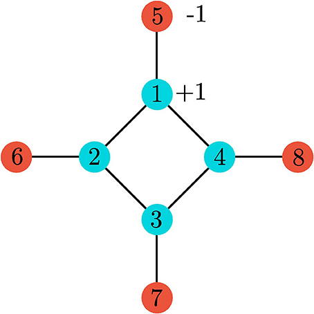
Figure 1. The eight spin graph from Boixo et al. [1]. Each spin is coupled to its neighbors along the graph with a +1 coupling such that the spins like to be aligned. In addition, the inner “core” spins have a magnetic field applied in the +z direction while the outer “ancilla” spins have a field applied in the -z direction.

The probability of finding the isolated (all down) state p_s is compared to the average probability of states from the 16-fold “cluster” of states, p_C. It is computed that classical simulated annealing finds an enhancement of p_s, i.e., p_s > p_C while quantum annealing both in simulation and running on the D-Wave machine finds a suppression p_s < p_C.

2.2. Annealing with 108 Spins

In Boixo et al. [2] 108 spins in the D-Wave computer are employed. Their connectivity is displayed in Figure 1 of that paper. Each connection is given a coupling of ± 1 at random. 1000 random cases are studied, and for each case the machine is run 1000 times¹. The ground state energies calculated are compared to the correct answer, which can be found for cases of this size [10]. A histogram of the probabilities of successfully finding the correct answer is shown. The histogram has a bimodal distribution, with significant peaks at probability zero and probability one. The cases where the machine never finds the answer are “difficult” cases and the ones where it always finds it are “easy” cases. By comparison, classical simulated annealing shows a unimodal distribution with no, or nearly no, cases being either hard or easy. See Figure 2 in Boixo et al. [2].

3. Quantum Annealing is not Annealing

Is it surprising that results of the D-Wave experiments differ greatly from classical simulated annealing? And should this be considered evidence that the machine is quantum or more powerful than classical computation in some way? We argue here that the answer to these questions is “no.”

What is called “quantum annealing” is often compared to classical simulated annealing [11], or to physical annealing itself. Though both quantum annealing and simulated annealing are used to find lowest-energy configurations, one is not the quantum generalization of the other. More properly, quantum annealing should be considered quantum adiabatic ground state dragging.

Simulated annealing proceeds by choosing a random starting state and/or a high temperature, then evolving the system according to a set of rules (usually respecting detailed balance) while reducing the simulated temperature. This process tends to reduce the energy during its evolution but can, of course, become stuck in local energy minima, rather than finding the global ground state.

Quantum annealing, on the other hand, involves no randomness or temperature, at least in the ideal. Rather, it is a particular type of adiabatic evolution. Two Hamiltonians are considered: The one for which one desires to know the ground state H_f, and one which is simple enough that cooling to its ground state is easy, H_i. At the start of the process, the system is initialized to the ground state of H_i by turning on H_i and turning off H_f and waiting for thermal equilibration. Then H_i is gradually turned off while H_f is gradually turned on. If this is done slowly enough, the system will at all times remain in the ground state of the overall Hamiltonian². Then, at the end of this process the system will be in the ground state of H_f³. It remains to measure the ground state. For the problems considered in Boixo et al. [1, 2], the ground state is typically known to be diagonal in the z basis. Thus, a measurement need not introduce any randomness.

Since classical simulated annealing is intrinsically random and “quantum annealing” is not, the differences reported in Boixo et al. [1, 2] are not surprising. For the eight-bit suppression of finding the isolated state, two things could have happened: Either the ideal machine would find the isolated state always, or never. It happens that, due to the structure of the state, the ideal outcome is “never,” which is certainly a suppression. The bimodal distribution found for the 108-bit computations is also just what one would expect: In the perfect case of no noise either the calculation gets the correct answer or it does not. The outcome is deterministic so there should be exactly two peaks, at probability of success zero and one. Classical annealing, which begins from a random state on each run, is not expected to succeed with probability one, even for cases where the system is not frustrated.

The bimodality of the D-Wave results, in contrast to the unimodality of simulated annealing, can be seen as evidence not of the machine's quantumness, but merely of its greater reproducibility among runs using the same coupling constants, due to its lack of any explicit randomization. The simulated annealing algorithm, by contrast uses different random numbers each time, so naturally exhibits more variablity in behavior when run repeatedly on the same set of coupling constants, leading to a unimodal historgram. Indeed if the same random numbers were used each time for simulated annealing, the histogram would be perfectly bimodal. To remove the confounding influence of explicit randomization, we need to consider more carefully what would be a proper classical analog of quantum annealing.

If, as we have argued, classical simulated annealing is not the correct classical analog of quantum annealing, what is? The natural answer is to classically transform a potential landscape slowly enough that the system remains at all times in the lowest energy state. In the next section we give a model classical system and, by running it as an adiabatic lowest-energy configuration finder, demonstrate that it exhibits the same computational behavior interpreted as a quantum signature in Boixo et al. [1, 2].

4. The Model

The flux qubits in the D-Wave machine decohere in a time considerably shorter than the time adiabatic evolution experiment runs. The decoherence times are stated to be on the order of tens of nanoseconds while the adiabatic runtime is 5–20 ms [2]. For this reason, one would expect that no quantum coherences should exist. We therefore model the qubits as n classical spins (“compass needles”), each with an angle θ_i and coupled to each other with coupling J_ij = 0,± 1. Each spin may also be acted on by external magnetic fields h_i in the z-direction as well as an overall field in the x-direction B_X. The potential energy function is then given by

$\begin{array}{cc}{V}_{\text{Ising}}=-{\displaystyle \sum _i\cos }({\theta }_i)h_i-\frac{1}{2}{\displaystyle \sum _{i\ne j}\cos }({\theta }_i)\cos ({\theta }_j)J_{ij}& \left(2\right)\end{array}$

and

$\begin{array}{cc}{V}_{\text{trans}}=-{\displaystyle \sum _i\sin }({\theta }_i)B_x.& \left(3\right)\end{array}$

Compare these to Equations (1) and (2) in Boixo et al. [1].

The adiabatic computation is performed (or simulated) by running the dynamics while gradually changing these potentials from V_trans to V_ising over a time T according to

$\begin{array}{cc}V(t)=A(t)V_{\text{trans}}+B(t)V_{\text{Ising}}& \left(4\right)\end{array}$

with A(0) = B(T) = 1 and A(T) = B(0) = 0. The equations of motion are simply:

$\begin{array}{cc}\frac{d}{dt}{\theta }_i={\dot{\theta }}_i\text{and}\frac{d}{dt}{\dot{\theta }}_i=\frac{dV}{d{\theta }_i}.& \left(5\right)\end{array}$

It is straightforward to integrate this system of ordinary differential equations.

5. Results

5.1. Eight Spin Model

The simulated adiabatic dragging time T needs to be long compared to the fundamental timescales of the system. Since units have been omitted in Equations (2–5), these are of order unity. Using T = 1000 produces good results as shown in the next section. Figure 2 shows the results of simulating the classical model of the eight spins from Boixo et al. [1] When the total adiabatic dragging time T is long enough, the dynamics lead to a stationary state (red lines). The core spin is driven to θ = 0, corresponding to |↑⟩, and the ancilla spin to $\theta =\frac{\pi }{2}$, corresponding to |→⟩. All other core and ancilla states behave identically. The final state |↑↑↑↑→→→→⟩ lies in the space spanned by the 16 cluster states. Within this space the ancilla spins are free to rotate as they contribute nothing to the energy provided the core states are all |↑⟩. Since there is nothing to break the symmetry of the initial all |→⟩ configuration, this is the final state they choose. This behavior is robust to added noise (blue lines). However, when the dragging time T is too short, the long-time behavior is not a stationary state (black lines).

FIGURE 2

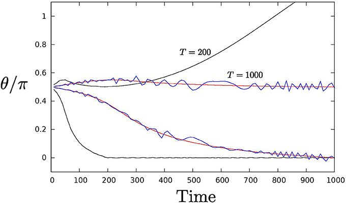
Figure 2. Results for eight spin model. Three runs are shown. In each case the angle θ of a representative core spin and ancilla spin are shown as a function of time. The core spins are all driven to θ = 0 while the ancilla spins are ideally driven to θ = Π/2. (1) The red lines show a case with no noise and with adiabatic drag time T = 1000. (2) The blue lines have added noise again with T = 1000. The noise was simulated by applying random kicks uniformly distributed between ± 0.02 to the angular velocities $\dot{\theta }$ of the spins at t = 10, 20, …. (3) The black lines have no noise but T = 200 (the evolution continues after the adiabatic drag is complete. It is easily seen the ancilla spin has been driven too fast and winds up with some kinetic energy (the slope is not zero for t > T).

5.2. 108 Spins

For this case we programmed 108 spins with the same connectivity and same random ± couplings as in Boixo et al. [2] Running our classical compass model simulation with no noise and a dragging time T = 1000 results in a perfect bimodal distribution. For about 2/3 of the cases the optimal answer was found always, and for the remaining 1/3 it was found never (since the machine is deterministic it is only necessary to run each case once).

We show in Figure 3 the results of running a simulation of the classical compass model with with noise. For the same 1000 sets of couplings, 100 noisy runs were performed and a histogram of success probabilities results. The bimodal distribution is maintained. We compare to Figure 2 in Boixo et al. [2] The qualitative nature of the bimodal signatures found is insensitive to the details of the noise so more realistic noise models would give similar behavior. Note also that the noise seems to help find the ground state, as in 920 of the 1000 cases the ground state was found at least once in 100 trials. This suggests that noisy adiabatic dragging picks up some of the benefits of classical simulated annealing, avoiding being “stuck” with either always or never finding the ground state.

FIGURE 3

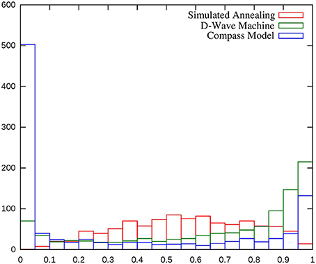
Figure 3. Results of 1000 spin glass instances, each run 100 times on a noisy simulation of the classical compass model with T = 1000. A bimodal distribution is observed, with a clear separation between easy and hard instancesd with high and low success probabilities respectively. The noise applied was random kicks to each $\dot{\theta }$ at t = 10, 20, …, 1000 uniformly chosen between ± 0.0015. The results are compared to the experimental data of Boixo et al. [2] and to an illustrative run of simulated annealing.

6. Conclusions

We have argued that quantum annealing and simulated annealing are very different procedures. The deterministic nature of quantum annealing leads to rather different behaviors than the random processes of simulated annealing. However, other deterministic procedures can also lead to behavior very similar to that observed in the D-Wave device. Our classical model reproduces all the claimed signatures of quantum annealing. We recommend using the term “ground-state adiabatic dragging” or simply “adiabatic computation” for such nonrandom processes.

Note that in Johnson et al. [12], under highly diabatic conditions, evidence was shown that the D-Wave device exhibits quantum tunneling. We emphasize that this does not constitute evidence for an essential use of quantum effects during adiabatic dragging and indeed an effectively classical model may well capture the physics and computational behavior seen in Boixo et al. [1, 2]. Tunneling is a possible additional path for a system to anneal into a lower energy state without needing enough energy to cross a potential barrier. If the decoherence is such that each spin is projected into a local energy eigenstate, then in the adiabatic limit, where each spin is at all times in its local ground state, tunneling locally can be of no assistance. The tunneling in Johnson et al. [12] is indeed only shown locally.

Furthermore, there is nothing preventing the implementation of our simulated compass model in hardware. It would be possible to build an analog classical machine that could simulate it very quickly, but it would be simpler to use a digital programmable array with one processing core per simulated spin. Since each spin requires knowledge of at most six of its neighbors along the connectivity graph, the algorithm can be easily parallelized. A 108 core computer specialized to running our algorithm could easily run hundreds or thousands of times faster than simulating it on a desktop computer, and could be built for modest cost using off-the-shelf components. Similarly, any classical physics can be efficiently simulated on a classical machine.

This is not to suggest that simulating classical physics directly on a classical computer is a good way to solve optimization problems. Classical simulated annealing [11] and other heuristic techniques have been extremely successful, and can also be very fast on special-purpose hardware. It is shown in Boixo et al. [2] that simulated annealing is competitive with the D-Wave One machine even on desktop CPUs (this has expanded on in great detail including new experiments on the D-Wave Two processor [13]). Stronger evidence of both quantumness and a resulting algorithmic speedup is needed before quantum adiabatic computers will have proved their worth.

7. Postscript

In the year since the original posting of this work on the quantum physics archive (arxiv.org), much has happened. The original preprint on which we were commented have been published [14, 15] and [15] in particular was updated to incorporate to some of our criticisms, also discussed in Boixo et al. [16] The main point of the response was that our model captured the bimodality, but not more subtle features of the data. An improved version of our model addressing these details appears as Shin et al. [17] This has also been responded to and re-responded to Vinci et al. [18] and Shin et al. [19] The current status of the question is that for a broad range of parameter space there is a simple classical model that captures the D-wave machine's input-output behavior. There is also a corner of parameter space where this model fails to reproduce certain aspects of the input-output behavior that a quantum master equation does capture. This quantum master equation fails to capture other aspects of the machine's behavior which the classical model does reproduce. As is to be expected for a complex system, there is no known model, either classical or quantum, that captures all aspects of the machine. We are gratified that our modest model has stimulated a more careful study of D-Wave's machine.

Conflict of Interest Statement

The authors declare that the research was conducted in the absence of any commercial or financial relationships that could be construed as a potential conflict of interest.

Acknowledgments

The authors thank Charles H. Bennett, Jay Gambetta, Mark Ritter, and Matthias Steffen for helpful comments on our manuscript.

Footnotes

1. ^They also look at what happens with fewer than 108 spins, so the total number of experiments they performed is actually much larger.

2. ^If the ground state is degenerate at some point during the process then this may not be true.

3. ^Of course, “slowly enough,” depends on the gapbetween the ground state and other nearby energy eigenstates. If the system is frustrated, there are many such states and the evolution must proceed exponentially slowly, just as frustration hinders classical simulated annealing. Though it has often been suggested that quantum annealing is a panacea, whether it can outperform classical simulated annealing in such cases is unknown.

References

1. Boixo, S, Albash, T, Spedalieri, FM, Chancellor, N, and Lidar, DA. Experimental signature of programmable quantum annealing. (2012) ArXiv:1212.1739. Available online at: http://arxiv.org/abs/1212.1739

Pubmed Abstract | Pubmed Full Text

2. Boixo, S, Ronnow, TF, Isakov, SV, Wang, Z, Wecker, D, Lidar, DA, et al. Quantum annealing with more than one hundred qubits. (2013) ArXiv:1304.4595. Available online at: http://arxiv.org/abs/1304.4595

3. Farhi, E, Goldstone, J, Gutmann, S, Lapan, J, Lundgren, A, and Preda, D. A quantum adiabatic evolution algorithm applied to random instances of an NP-Complete problem. Science (2001) 292:472–5. doi: 10.1126/science.1057726

Pubmed Abstract | Pubmed Full Text | CrossRef Full Text

4. Aharonov, D, van Dam, W, Kempe, J, Landau, Z, Lloyd, S, and Regev, O. Adiabatic quantum computation is equivalent to standard quantum computation. SIAM J Comput. (2007) 37:166–94. doi: 10.1137/S0097539705447323

CrossRef Full Text

5. Shor, PW. Fault-tolerant quantum computation. In: Proceedings of the 37th Symposium on Foundations of Computing, FOCS 1996. (1996) p. 56–65.

6. Barahona, F. On the computational complexity of Ising spin glass models. J Phys. (1982) 15:3241.

7. Bansal, N, Bravyi, S, and Terhal, BM. Classical approximation schemes for the ground-state energy of quantum and classical ising spin hamiltonians on planar graphs. Quant Info Comput. (2009) 9:701–20.

8. Harris, R, Berkley, AJ, Johnson, MW, Bunyk, P, Govorkov, S, Thom, MC, et al. Sign- and magnitude-tunable coupler for superconducting flux qubits. Phys Rev Lett. (2007) 98:177001. doi: 10.1103/PhysRevLett.98.177001

CrossRef Full Text

9. Mooij, JE, Orlando, TP, Levitov, L, Tian, L, van der Wal, CH, and Lloyd, S. Josephson persistent-current qubit. Science (1999) 285:1036–9. doi: 10.1126/science.285.5430.1036

Pubmed Abstract | Pubmed Full Text | CrossRef Full Text

10. Mooij, JE Spin glass server. Available online at: http://www.informatik.uni-koeln.de/spinglass/

11. Kirkpatrick, S, Gelatt, CD, and Vecchi, MP. Optimization by simulated annealing. Science (1983) 220:671–80. doi: 10.1126/science.220.4598.671

Pubmed Abstract | Pubmed Full Text | CrossRef Full Text

12. Johnson, MW, Amin, MHS, Gildert, S, Lanting, T, Hamze, F, Dickson, N, et al. Quantum annealing with manufactured spins. Nature (2011) 473:194–8. doi: 10.1038/nature10012

Pubmed Abstract | Pubmed Full Text | CrossRef Full Text

13. Rnnow, TF, Wang, Z, Job, J, Boixo, S, Isakov, SV, Wecker, D, et al. Defining and detecting quantum speedup. Science (2014) 345:420–4. doi: 10.1126/science.1252319

Pubmed Abstract | Pubmed Full Text | CrossRef Full Text

14. Boixo, S, Albash, T, Spedalieri, FM, Chancellor, N, and Lidar, DA. Experimental signature of programmable quantum annealing. Nat Commun. (2013) 4:2067. doi: 10.1038/ncomms3067

Pubmed Abstract | Pubmed Full Text | CrossRef Full Text

15. Boixo, S, Ronnow, TF, Isakov, SV, Wang, Z, Wecker, D, Lidar, DA, et al. Evidence for quantum annealing with more than one hundred qubits. Nat Phys. (2014) 10:218–24. arXiv:quant-ph/0703264.

16. Boixo, S, Ronnow, TF, Isakov, SV, Wang, Z, Wecker, D, Lidar, DA, et al. Comment on: “Classical signature of quantum annealing.” (2013) ArXiv:1305.5837. Available online at: http://arxiv.org/abs/1305.5837

17. Shin, SW, Smith, G, Smolin, JA, and Vazirani, U. How “Quantum” is the D-Wave Machine? (2014) ArXiv:1401.7087.

18. Vinci, W, Albash, T, Mishra, A, Warburton, PA, and Lidar, DA. Distinguishing classical and quantum models for the D-Wave device. (2014) ArXiv:1403.4228.

19. Shin, SW, Smith, G, Smolin, JA, and Vazirani, U. Comment on: “Distinguishing classical and quantum models for the D-Wave device.” (2014) ArXiv:1404.6499.