 Saliou Faye
 Alban Lazar
 Bamol A. Sow
 Amadou T. Gaye1
- 1Laboratoire de Physique de l'Atmosphère et de l'Océan Simeon Fongung (LPAO-SF/ESP/UCAD), Dakar, Senegal
- 2Centre de Recherche Océanographique Dakar-Thiaroye (CRODT/ISRA), Dakar, Senegal
- 3Laboratoire d'Océanographie et du Climat: Expérimentations et Approches Numériques (LOCEAN/UPMC), Paris, France
- 4Laboratoire d'Océanographie, des Sciences de l'Environnement et du Climat (LOSEC/UASZ), Ziguinchor, Senegal
The climatological seasonal cycle of the sea surface temperature (SST) in the north-eastern tropical Atlantic (7–25°N, 26–12°W) is studied using a mixed layer heat budget in a regional ocean general circulation model. The region, which experiences one of the larger SST cycle in the tropics, forms the main part of the Guinea Gyre. It is characterized by a seasonally varying open ocean and coastal upwelling system, driven by the movements of the intertropical convergence zone (ITCZ). The model annual mean heat budget has two regimes schematically. South of roughly 12°N, advection of equatorial waters, mostly warm, and warming by vertical mixing, is balanced by net air-sea flux. In the rest of the domain, a cooling by vertical mixing, reinforced by advection at the coast, is balanced by the air-sea fluxes. Regarding the seasonal cycle, within a narrow continental band, in zonal mean, the SST early decrease (from September, depending on latitude, until December) is driven by upwelling dynamics off Senegal and Mauritania (15–20°N), and instead by air-sea fluxes north and south of these latitudes. Paradoxically, the later peaks of upwelling intensity (from March to July, with increasing latitude) essentially damp the warming phase, driven by air-sea fluxes. The open ocean cycle to the west, is entirely driven by the seasonal net air-sea fluxes. The oceanic processes significantly oppose it, but for winter north of ~18°N. Vertical mixing in summer-autumn tends to cool (warm) the surface north (south) of the ITCZ, and advective cooling or warming by the geostrophic Guinea Gyre currents and the Ekman drift. This analysis supports previous findings on the importance of air-sea fluxes offshore. It mainly offers quantitative elements on the modulation of the SST seasonal cycle by the ocean circulation, and particularly by the upwelling dynamics.
Introduction
The sea surface temperature (SST) is a crucial quantity for studies of both climate variability and marine ecosystem productivity. In the tropical Atlantic, as well as for the other tropical basins, SST exerts a significant influence on the climate of surrounding regions (e.g., [1, 2]). It is also a major indicator of the state of the marine environment relative to phytoplankton biomass needs, particularly for upwelling zone activity, and particularly for coastal upwellings [3]. One of the less studied zones is the Atlantic North-eastern Tropical Upwelling System (ANETUS, examined here from 7 to 25°N and 12 to 26°W). It is also one of the regions experiencing the largest SST seasonal cycle in the tropics. In this study, we propose to present and interpret the full spatial distribution of the processes driving the seasonal cycle of the SST, for the open ocean upwelling regime, as well as at the coasts.
Trade winds and the ITCZ generate large scale divergent Ekman transports, which force in the northern hemisphere a tropical upwelling system that continuously extends from Morocco to the mouth of the Guinea Gulf, and from the African coasts to mid and west Atlantic, depending on season [4, 5]. Considered from a basin-scale perspective, this system forces a cyclonic gyre circulation, the Guinea Gyre [e.g., 6], of which the Guinea Dome and the coastal West-African upwellings form the most eastern features [4, 7]. In this paper, we limit our study to the eastern part of the system, bounded in latitude by the Tropic of Cancer and the North Equatorial Counter-Current and in longitude by the Cape Verde Archipelago (CVA around 26°W) and African coasts. This area is marked by intense, seasonally dependent, off-shore and coastal primary production patterns of major economic importance. The coastal part of the upwelling system covers latitudes ranging from Morocco and Canary Islands to Senegal [8] and further south down to the Guinea Gulf. It forms the tropical part of the Canary Current Upwelling System (CCUS) down to Senegal, as well as the northern part of the Guinea Current Upwelling System that extends from Guinea coasts to the Gulf of Guinea. The CCUS is one of the four major eastern boundary upwelling systems with those of Peru-Chile, Benguela, and California.
Horizontal circulation is schematized Figure 1. To the west, the North Equatorial Current (NEC) and the Canary Current (CC) forms the eastern boundary of the North Atlantic subtropical gyre. Near-shore, a strong wind-induced coastal upwelling is active, its extension depending on season, and a density front develops that generates the coastal jet [9–11], also named Canary upwelling Current (CanUC) [12]. However, observations are lacking and its latitudinal extension to the south is uncertain, with some model studies showing it down to the Cape Verde peninsula (see dashed green arrow in Figure 1). South of the region, the circulation is dominated by the North Equatorial Counter-Current (NECC), which has a large seasonal cycle [13, 14]. It is located near 5°N in winter and reaches 10°N in summer. During this season, it continues north as the Mauritania Current (MC), which flows northward until about 20°N [15]. Offshore, the Guinea Dome (GD) is another important physical characteristic of the area, defined by a dome of the isotherms, and low hydrostatic pressure. It is centered in the southeast of the archipelago of Cape Verde, and intensifies in summer, at about 12°N, and 22–23°W. It is generated by upward Ekman pumping forced by the trade winds convergence [7, 17], and belongs to the Guinea Gyre, formed by the NEC and NECC in surface [4, 13]. It exist a link between the GD with the Atlantic Meridional Mode (AMM) which is related to the meridional migration of the Intertropical Convergence Zone (ITCZ) [18, 19].
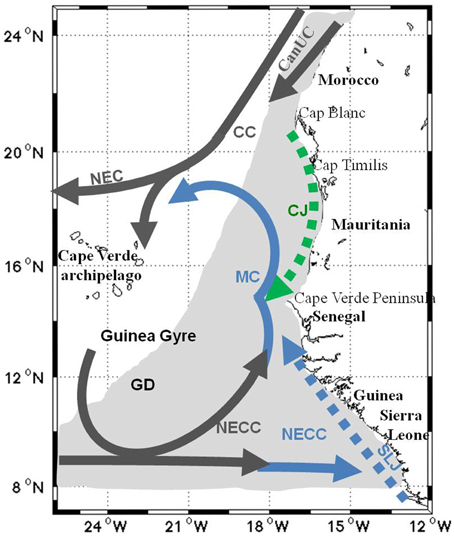
Figure 1. Map of the schematic surface circulation in the Atlantic North-eastern Tropical Upwelling System characterized by permanent currents (dark gray), seasonal currents in winter-spring (green), another seasonal currents in summer-autumn (blue) and upwelling area (gray shading). Dash line corresponds to currents not evidenced by in-situ measurement, but visible in circulation derived from altimetry. (adapted from [16])
Regarding SST in our region, the mechanisms that drive its seasonal cycle are not yet certain. Carton and Zhou [20] ocean model sensitivity experiments show that air-sea flux and wind stress forcing are of comparable importance away from the continent, whereas within a few degrees of the African coasts, the meridional stress becomes the main forcing. Yu et al. [21] on the other hand evidenced the very high correlation at large scale in the region north of 10°N between the SST time derivative and the net air-sea flux. The first study can be interpreted as an indication that advection and associated Ekman pumping are important for the region, and dominant at the coast. The second may suggest that they do not drive the seasonal cycle. More specifically, the upper heat content at ~12°N and few specific longitudes, within the Guinea Dome in particular, was studied by Yamagata and Iizuka [7]. They found that the summer subsurface cooling is explained comparably by horizontal and vertical advection. However, these results pertain to the upper thermocline doming, since SST increase in fact during the GD development. A proper (ML in the following) heat budget for the climatological SST seasonal cycle of the western part of our domain, was carried out by Foltz et al. [22] from observations and reanalysis products. They find also that air-sea fluxes drive the cycle, and suggest, from the heat budget residual, that vertical mixing damps it.
Regarding coastal patterns, their seasonal variability has been the subject of studies based on upwelling indices, calculated from in situ measurements [8] or satellite observations of SST [23]. They nevertheless often lack a robust heat budget analysis for the SST, that could provide clear physical interpretations of the SST changes. Along African coasts, an important issue for the system is how much upwelling forces SST, and how long does its effect last during the year. For example, Santos et al. [24], using a temperature-based estimate suggest that if the upwelling is persistent throughout the year, with a peak in autumn and spring, between 21 and 32°N, it would in contrast be restricted to winter-spring within the 12° and 20°N latitude band. These authors hypothesize that the turn of the summer monsoon winds would advect warm waters northward along-shore. One may wonder how much it contributes to the SST warming and what are the upwelling real cycle and effects, since a wind-derived proxy indicates rather that the latter persists in summer from 15 to 20°N, albeit weaker [e.g., 3]. Furthermore, air-sea heat fluxes could potentially also explain this summer evolution. In fact, within the coastal Mauritania and Senegal upwellings, even the first order balance between horizontal advection, subsurface heat fluxes and air-sea fluxes is unknown. This deserves to be checked in an Ocean Global Circulation Model (OGCM) and tested to the East, where the upwelling is stronger. A model study like the one we present here, despite its inherent uncertainties due to forcings and model errors, can offer complementary results. In this paper, we provide some quantitative elements of answer to the various uncertainties existing about the ocean dynamics and the control of the SST seasonal changes in the ANETUS, with observations and an OGCM. The focus is on the regimes of heat budget, and the processes that drive them, in particular the turbulent vertical mixing, hardly quantifiable from observations only and not yet analyzed per-se in the literature.
The article is structured as follows. The data and methods are presented in Section Data and Methods. In Section Choice of Relevant Time-average Periods, we present the general circulation features in observations and the simulation. Then we analyze in Section The Mixed Layer Heat Budget the spatial structures of oceanic and atmospheric contributions to the heat budget, and detail their temporal variations for continental and open-ocean sub-domains. Results are then summarized and discussed in Section Summary and Discussions.
Data and Methods
Observations
The NOAA AVHRR OISST SST at 25 km resolution is monthly averaged to produce the climatology for the period 1988–2000 that we use to evaluate model SST. For the circulation, OSCAR surface currents are used. They are representative of total geostrophic and wind-driven circulation over the first 15 m depth layer and are available on a horizontal grid of 1/3° × 1/3° [25]. Geostrophic currents are provided on a 1/3° × 1/3° spatial grid by AVISO. We constructed monthly-climatologies of surface circulation, with both products for the period 1993–2000, close to that of the climatological forcing used to run our model. Climatological wind stress is provided by the DFS4 forcing set (see further description in Numerical Model), and derived from the ERA40 reanalysis winds, which assimilated the QuickSCAT winds. The Ekman vertical velocities associated with the climatological winds are estimated using the Ekman transport divergence formula. Null cross-shore transport at the coast is enforced by setting the wind stress to zero at each land point. Note that both the coastal pumping and offshore Ekman pumping are computed with this formula. Mixed layer depth (hereafter MLD) is given by the monthly climatology from De Boyer Montégut et al. [26] on a 2° × 2° horizontal resolution. We retained the product based on a temperature threshold of 0.2°C, since the density-based product has a much less dense cover in our area of study. Thermocline depth is evaluated using the monthly climatological WOD05 hydrological dataset on a 1° × 1° latitude–longitude grid.
Numerical Model
The NEMO modeling system [27] is based on the global OGCM OPA, which solves the primitive equations on an Arakawa C grid, with a second-order finite difference scheme. It assumes the Boussinesq and hydrostatic approximations, and assumes incompressibility. In the present study, we use the regional configuration for the tropical Atlantic ATLTROP025, derived from the global DRAKKAR configuration ORCA025-G70 [28] with an extension limited to 30°N and 30°S. The horizontal resolution is 0.25° × 0.25°. Realistic bottom topography and coastlines are derived from ETOPO2. The vertical dimension is resolved by 46 z-levels with a vertical mesh size ranging from 5 m in the upper 30–250 m at depth. Most relevant elements of the parameterization are the following. A horizontal biharmonic operator is used for the diffusion of horizontal momentum, with a viscosity coefficient (background value of −1.5 10−11 m4.s−2) varying as δx3 (δx the horizontal grid size). Diffusion of temperature and salinity uses a Laplacian operator rotated along isopycnals, with a coefficient decreasing proportionally to the grid size (starting at 300 m2.s−1 at the equator). Vertical mixing of momentum and tracers is computed using a second-order turbulence kinetic energy closure model described in Madec [27]. Lateral boundary conditions are provided by the global run ORCA025-G70. For surface forcing, we use the DRAKKAR DFS4 6-hourly global forcing datasets [29]. To calculate latent and sensible heat fluxes, the CORE [30] bulk formulae algorithm is used, with surface atmospheric state variables derived from the ERA40 reanalysis and ECMWF analysis after 2002 (air temperature, humidity and winds at 10 m). Corrections are performed on these input fields to correct temporal discontinuities and yield better agreement with some recent high quality data. Radiation fluxes are based on the CORE v1 dataset, using a corrected ISCCP-FD radiation product [31]. For these experiments, we forced the model for thirteen years with climatological weekly fields averaged over the period 1988–2000. The 5-day mean outputs were averaged climatologically over the last year of simulation. It is worth to stress out that in order to study a climatological state closer to the observational one, it would be more rigorous to analyze a simulation of the same period as the observations, forced by the non-climatological fields. Such a simulation however, including heat budget diagnostics described below, was not yet realized at time of our study. It will be worth in the future to verify our conclusions with such a run.
For the present study, we derived off-line a number of quantities from the model outputs. In particular we estimated surface horizontal currents from the total SSH using the geostrophic equation and assumed they did not vary with depth over the ML. The model computes MLD using a density threshold of 0.01 kg.m−3, and we use this output throughout the paper. For the validation section however, we also estimated MLD offline with the same threshold of 0.2°C, although the online computation (not available) would have been more comparable.
Diagnostics
In this study, we follow the approach used by Vialard and Delecluse [32] and by Peter et al. [33] and Jouanno et al. [34] where the ML temperature equation is partitioned as follows:
with
Here, the brackets represent a vertical integration over the MLD, T is the temperature, and w are the horizontal and vertical currents, Kz is the vertical mixing coefficient, h is the MLD, and Dl(T) is the lateral diffusion operator. Q* and Qs are the non-solar and solar components of the total heat flux, and fz = h is the fraction of the solar shortwaves that reaches below the MLD. Capital letters underneath terms are used, respectively, as short-hands for horizontal advection, horizontal diffusion associated with unresolved horizontal turbulent processes, vertical advection, vertical turbulent mixing at the ML base and air-sea fluxes. A last term res, computed as a residual, corresponds to the entrainment at the ML base. Note that we have checked that the latter is always largely negligible in our area.
In the following work, horizontal advection and vertical mixing always dominate the ocean contribution to the heat budget. For the sake of synthesis, we chose to group the ocean terms in horizontal and vertical processes terms. The first is the sum of lateral diffusion and horizontal advection contributions (A+B), and the second the sum of vertical advection, vertical mixing and entrainment (C+D+res). These group components have been checked individually relative to the others, and are discussed separately when they are significant. Term E corresponds to the net air-sea flux effect. To quantify the relative importance of terms, we compute their ratios. In the section dedicated to time-averages, we computed ratios of time-averaged group of terms, to emphasize their relative time-mean effects, whereas in the following section focusing on time-variations, we instead present the ratios of 5-day outputs. Differences between both computations are of second order and not relevant to discuss in this study.
Results
Choice of Relevant Time-average Periods
In order to distinguish time periods relevant for studying time-averages of the heat budget terms with a focus on the ocean contribution, Figure 2 presents the Ekman upwelling and SST cycle averaged longitudinally from the coast to 18°W. The former is computed as the total Ekman transport divergence, including that of the alongshore grid-points. It first evidences the well-known latitudinal transition from a strongly varying upwelling at low latitudes to a more stable northern regime [e.g., 24, 35]. On both sides of approximately latitude 18°N, the Ekman pumping peaks occur out of phase, in agreement with Lathuilière et al. [3], due to the seasonal shift of the inter-tropical convergence. Low latitudes are marked by an intense winter regime, followed by a relaxation phase in summer, in particular off Senegal (10–16°N). North-Mauritania and south-Morocco latitudes (18–22°N) experience a peak in summer. Based on the strongest Ekman pumping and seasonal SST changes, we identify a first period from November to May, characterized globally by lowest or decreasing SST (so-called cooling period, (hereafter CP), and a warming period (hereafter WP) from June to October characterized by increasing or high SST. Next section, we describe the CP and WP general circulation and SST change patterns in the observation-derived products, and validate the simulation.
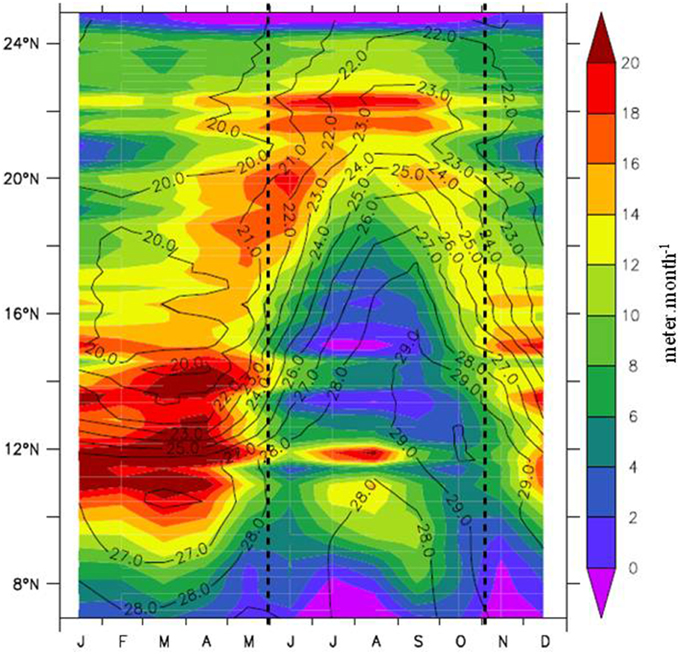
Figure 2. Latitude-time Hovmöller plot along the coastal region (averaged from the coast to 18°W) of the seasonal cycles of Ekman pumping (shading, m.month−1) and SST (contours, °C). Dash lines separate CP (November–May) and WP (June–October) periods.
SST Variations and Mixed Layer Depth
Figure 3A displays observed SST variations for CP (computed as the SST difference between the end and the beginning of the period). They exhibit an extremum (−0.7°C.month−1) located around (18°N, 18°W) off Mauritania coast. A second relative extremum (−0.6°C.month−1) is located close to shore near 14.5°N, just south of the Cape Verde Peninsula in the southern Senegal upwelling center [36]. The model presents a more noisy structure (Figure 3B), due to the shorter length of average period relative to the observations. This being said, the large-scale patterns of the model are comparable to those of the observations, with only a slight underestimation of the cooling (~0.2°C.month−1) near the coast from 14° to 20°N. The large-scale structure of the temperature change during WP is very similar with a sign reversal and a somewhat more rapid evolution (maxima ~1°C.month−1, Figure 3C). The model is able to simulate this distribution although the area of largest warming tends also to be shifted a few degrees to the southwest. Nearshore, the highest differences reach comparable negative values as during CP (~ -0.2°C.month−1) from 15 to 22°N (Figures 3C,D). Figure 3 also shows the SST and MLD fields, which are essential to the heat budget analysis. The model SST suffers from a warm bias, generally between 0.5 and 1°C. The model MLD is 10–30 m too deep during CP and about 5 m too shallow during WP. Because there are little observations in the region, uncertainties are large particularly for MLD, and we consider the model sufficiently realistic.
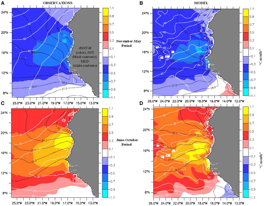
Figure 3. SST trend (color, in °C.month−1), SST (black contour, in °C) and mixed layer depth (white contour, in m), averaged over CP (November–May, top) and WP (June–October, bottom); left (A,C) for observations and right (B,D) for simulation.
Upwelling and Stratification
To better understand the effect of the wind-driven circulation on the ML heat budget, Figures 4A,C present the Ekman pumping patterns for CP and WP. To compare to the model, we present the maximum value of the model vertical velocities found between the surface and the base of the thermocline (Figures 4B,D). The spatial extent of the upwelling appears remarkably stable between the two seasons, and this is also verified with the monthly values (not shown). The strongest upwelling velocities are located nearshore north of ~10°N, where they reach values of the order of 100 (resp. 50) m.month−1 during CP (resp. WP). Offshore, upwelling velocities display one order of magnitude lower values. They are associated with the trade winds curl and decrease gradually westward, more rapidly in the north than south, where they are responsible for the presence of the Guinea Dome. In the lee of the Cape Verde Islands, atmospheric island wake effect creates an upwelling–downwelling dipole patterns with typical scales of ~100–200 km [37]. Regarding intensities derived from observations they most vary from CP to WP near the coasts, in the north (by a factor of ~1.5), and much considerably south of 15°N (factor of ~0.25) in support of Lathuilière et al. [3] estimate. For both periods the model is at large scale in good agreement with Ekman pumping estimates. This validates the model vertical dynamics, and indicates that Ekman pumping corresponds in general well to the maximum upper ocean vertical velocity. The most remarkable differences occurs nearshore over the wide shallow continental shelves of the Banc d'Arguin (~20°N) and south of Senegal (~14°N). Vertical velocities comparable to Ekman pumping are found west of the coast there. This is explained by the fact that, due to the shallow plateau there, bottom friction disturbs the surface Ekman layer and classical Ekman theory does not apply. The Ekman divergence is then fully developed further offshore where the plateau is deep enough [see 38, 39].
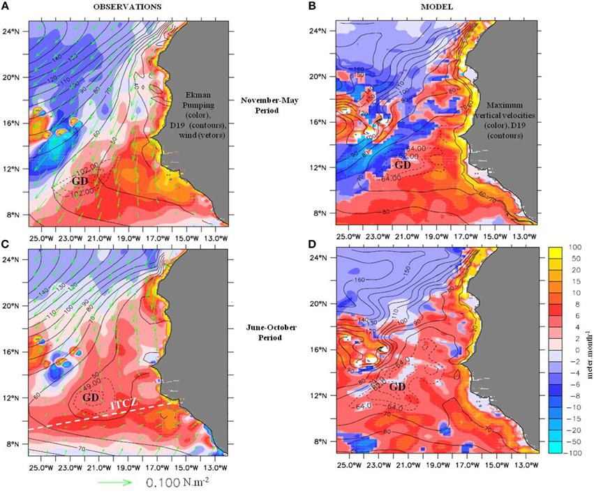
Figure 4. Ekman pumping (shading, m.month−1), 19°C isotherm depth (black contours, m) and wind stress (green vectors, N.m−2) from observations, averaged over (A) the CP(November–May) period, and (C) WP (June–October) period. Maximum vertical velocities between surface and thermocline (shading, m.month−1) and 19°C isotherm depth (black contours, m) for the simulation, averaged over (B) the November-May CP period, and (D) June–October WP period. GD, Guinea Dome.
Since the thermocline depth reflects the stratification, which controls the turbulent heat fluxes at the ML base, it is important to validate its distribution. The 19°C isotherm depth is shown as a proxy. Modest differences in the position and shape of the GD (in subsurface, it is particularly visible near 100 m in observations (D15) and about 60 m in the model; Figures 4A,B) in particular are noticeable, and model values are deeper by about 20 m, possibly as a consequence of an overly diffuse thermocline, a common bias in OGCM.
Horizontal Surface Circulation
We present total and geostrophic surface currents on Figure 5. The major geostrophic currents in the region are well represented by the model (in black). The CC, NEC, CanUC, NECC and circulation around the GD are visible during the two periods. The CC exhibits an important seasonal variability with a strengthening during WP in association with stronger winds in the north (Figures 5B,D). A similar seasonal cycle is found in the observations but an important difference should be noted: the observation derived CC appears quite relatively patchy, as appear the total currents. The model westward circulation is comparatively less complex, in particular during CP where the westward flow is quite uniform north of 16°N. In the latitude range 7–16°N, the offshore flow is more seasonally variable. The MC and GD recirculation are both very clear in observed and simulated geostrophic currents. We also note the intense well-organized westward ageostrophic flow spanning 13–16°N east of the CVA in the model (note the weak geostrophic currents in both panels). This flow is coherent with the southward wind forcing (see Figure 4A). It is however not visible in the OSCAR reconstruction, which is weaker and noisy. During WP the NECC seems slightly reinforced by Ekman drift in the model and observations and turns into the Guinea Current to the South and into a northern circulation branch, particularly intense at the coast. The turning point appears to be the slope change of Sierra Leone coastline (~8.5–9°N). Before this northern current becomes the MC, we propose to name it the Sierra Leone Jet (SLJ). The difficulty for observations to represent the circulation features in this region is well-known and due to sparse measurements [40], which pose difficulties to validate satellite-derived products and in particular in regions of coastal distortions of the satellite estimates. We shall be cautious when presenting the advective terms in the heat budget, but do not a priori disqualify the modeled circulation where it disagrees with OSCAR and AVISO, particularly nearshore.
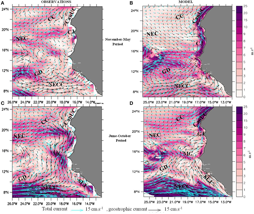
Figure 5. Horizontal surface currents averaged over the CP (November–May, top) and WP (June–October, bottom) for observation-derived (A,C) and simulated (B,D); intensity of the total surface current (shading, m.s−1), total (blue vectors) and geostrophic component (black vectors).
The Mixed Layer Heat Budget
In this section, we analyze the terms of the heat budget. We first analyze the spatial structures of the mains terms in order to evidence better their physical origins. The annual mean is presented, and then the CP and WP time-means, to take into account the cycle of the wind-driven upwelling activity, Then zonal averages are eventually examined for eastern and western sub-domains in function of time, in order to determine which processes are driving the time-variations of the SST.
Annual Mean
Figure 6 shows the annual mean of ocean effects, and its two components, the horizontal and vertical processes. Since the sum of air-sea heat fluxes and ocean effects is equal to the annual heat storage, which is negligible in the model climatology, the net heat flux effect is the opposite of the ocean effect. Meridionally, there is a contrast between an ocean warming south of roughly parallel 12°N, and a cooling effect north of it. Zonally, contributions are maximum at the coast with values of up to −5°C.month−1, and decrease abruptly westward by an approximate factor of five over a few degrees of longitude (Figure 6A). For the sake of differentiating sub-domains, we chose the longitude 18°W to separate regimes marked by high values dominated by coastal dynamics, and those with low values controlled by open-ocean circulation. In the west of the domain, CVA forms a specific sub-domain of intermediate or elevated intensities, which would require specific discussions out of scope of this paper.
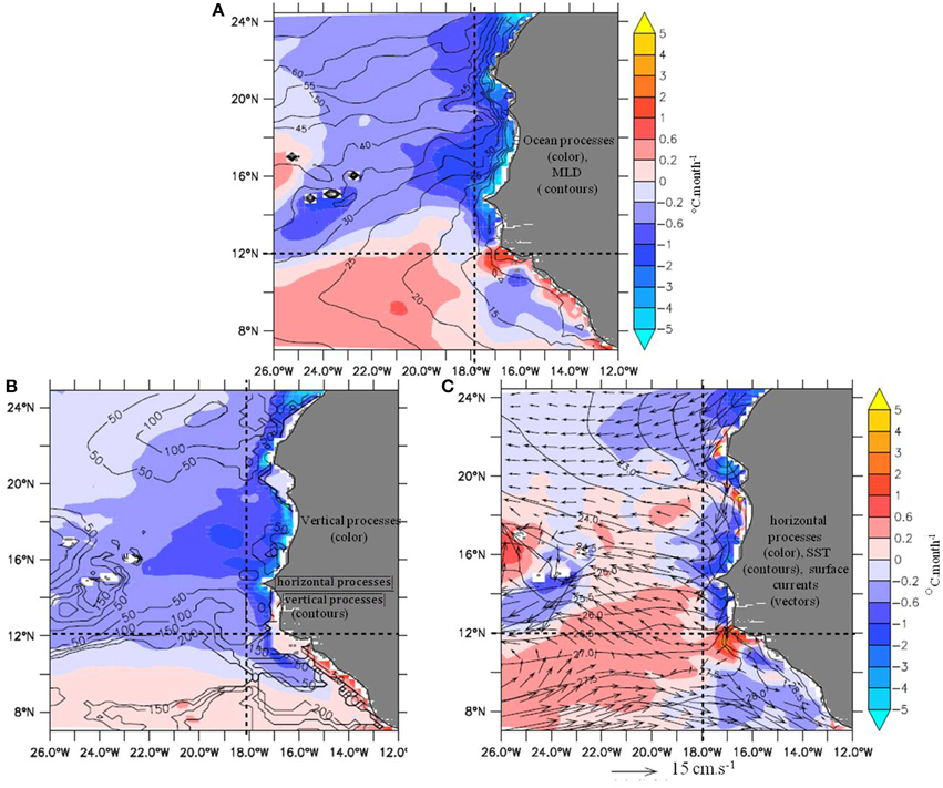
Figure 6. Annual average of the various oceanic processes contributing to the mixed layer heat budget. (A) Total oceanic trend (shading, °C.month−1), and mixed layer depth (MLD, black contours, m), (B) trend associated with vertical processes (sum of vertical advection, vertical diffusion at the base of the mixed layer and RES, shading, °C.month−1) and ratio of horizontal processes over vertical processes (contour every 50, 100, 150, and 200%) and (C) horizontal processes (sum of the horizontal advection and lateral diffusion, shading, °C.month−1), SST (black contour, °C) and surface currents (vectors). Vertical and horizontal dotted lines delimit regimes within the region.
Figures 6B,C show that the meridional contrast is explained by differences in the vertical and horizontal processes. North of ~12°N, vertical processes cause an expected general cooling through vertical exchanges with colder subsurface waters. It is worth noting that they prevail over the horizontal ones by a factor of about two in large parts of the domain, while both effects reach comparable amplitudes off Morocco and Cape Verde Islands. South of 12°N, a remarkably vast warming effect, albeit weak except along-shore, is sustained by vertical processes, which indicate the influence of temperature inversions, as it will be demonstrated in WP analysis. The location corresponds to patterns of barrier layers associated with ITCZ rainfall [41] that allow for the presence of temperature inversions. The ocean warming effect is however dominated by advection of warm waters poleward by the NECC (Figure 6C), except alongshore where currents are weak and SST is warmed up also by temperature inversions (Figure 6B). Note that 12°N corresponds to the GD latitude. This shows that, in annual mean, the ocean cools the GD SST in its northern half, but warms it in its southern part. Overall, south of 12°N, horizontal advection dominates vertical processes (Figure 6C), but for the remaining part of the region, heat exchanges with the thermocline cools the domain SST with a larger or comparable amplitude than horizontal currents effect (Figure 6B).
November–May Cooling Period
As we will see, during CP, the ocean contribution displays the larger negative signals, whereas during WP, it is the net air-sea flux contribution. Thus we start the CP analysis with the interpretation of the ocean terms, and then will study the WP starting with the investigation of the air-sea fluxes effects. During CP the total ocean contribution is close to its annual mean (Figures 6A, 7A). The ratio of time-mean contributions of horizontal and vertical processes indicates that the latter have a larger effect on the SST cooling, next to the continent, as well as to the west in the latitude band 12–20°N. Compared to the annual mean, the vertical processes cause a stronger (weaker) cooling in the 12–18°N (18–24°N) coastal upwelling band (Figure 7B), evidently associated with the latitudinal structure of the seasonal Ekman pumping changes. It explains the same pattern in the total ocean contribution.
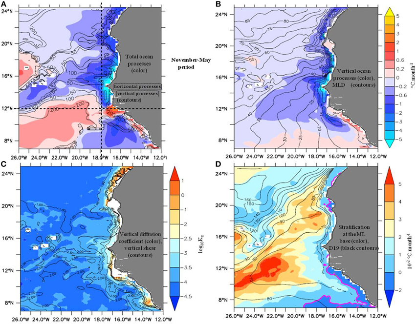
Figure 7. Model oceanic trends averaged over CP averaged over the CP period. (A) Total ocean effect (shading, °C.month−1) and ratio of contributions of horizontal processes over vertical processes, each in time-average (black contours), (B) Vertical processes effect (shading, °C.month−1) and mixed layer depth (MLD, black contours, m), (C) vertical diffusion coefficient (shading, m2.s−1) and square of the vertical shear at the base of the ML (black contour, s−2), and (D) vertical temperature gradient at the base of the ML (shading, °C.m−1) and the 19°C isotherm depth (black contours, m).
To detail further vertical cooling, we first note that it is by far dominated by vertical diffusion (not shown). Then by computing off-line the latter with model outputs of vertical diffusivity (Kz), temperature and MLD (see formula of D in Equation 1) we reproduced satisfyingly its pattern (not shown). Hence we examine diffusivity and vertical temperature gradient at the ML base. It appears that the maximum intensities along-shore is due to stronger vertical diffusivity there (Figure 7C), not to vertical temperature gradients which are weak compared to offshore (Figure 7D). We interpret this as a manifestation of coastal upwelling dynamics which generates intense current shear near the base of the mixed layer ML (Figure 7C, contours). It thereby enhances turbulence levels, simulated by large Kz. Intense coastal upwelling tends also to erode upper ocean stratification, relative to the moderate open-ocean upwelling to the west. To complete the explanation of this zonal variation, it is important to say that the MLD zonal pattern amplifies significantly the effect of the diffusive flux at the coast. Indeed, MLD, which enters the diffusive flux term in the denominator, is shallower at the coast by a factor of 1.5–2 relative to further west. Far from the continent, west of 18–19°W, the cause of relative high vertical diffusion is opposite. The vertical temperature gradients at the mixed layer ML base reach maximum intensities, about five times larger than nearshore (Figure 7D), explaining the vast and moderate diffusion pattern. The Guinea Gyre upwelling lifts gently the isotherms and maintains a strong stratification, maximal at the GD location. On the other hand, Kz is smaller (Figure 7C), in relation to weaker shear of horizontal current compared to nearshore.
Regarding the horizontal processes contribution (Figure 8A), it also appears similar to its annual mean (Figure 6C). It is essential to the model for redistributing heat horizontally, and modulating the 1D vertical upwelling dynamics. We first note that horizontal advection prevails largely over horizontal diffusion (not shown). Then in order to interpret advective effects, we estimated off-line the geostrophic and ageostrophic components of the horizontal advection term. To do so, surface geostrophic and ageostrophic currents were calculated (the latter as the total minus the geostrophic currents), and then used for computing scalar products with SST gradients. Figures 8B,C show that both contributions are most intense in the vicinity of coastlines, due to maximum SST gradients and generally more intense currents. They often partly oppose each-other, especially close to the continent, where geostrophic flow compensate partially, in addition to coastal upwelling, the mass imbalance generated by Ekman divergence.
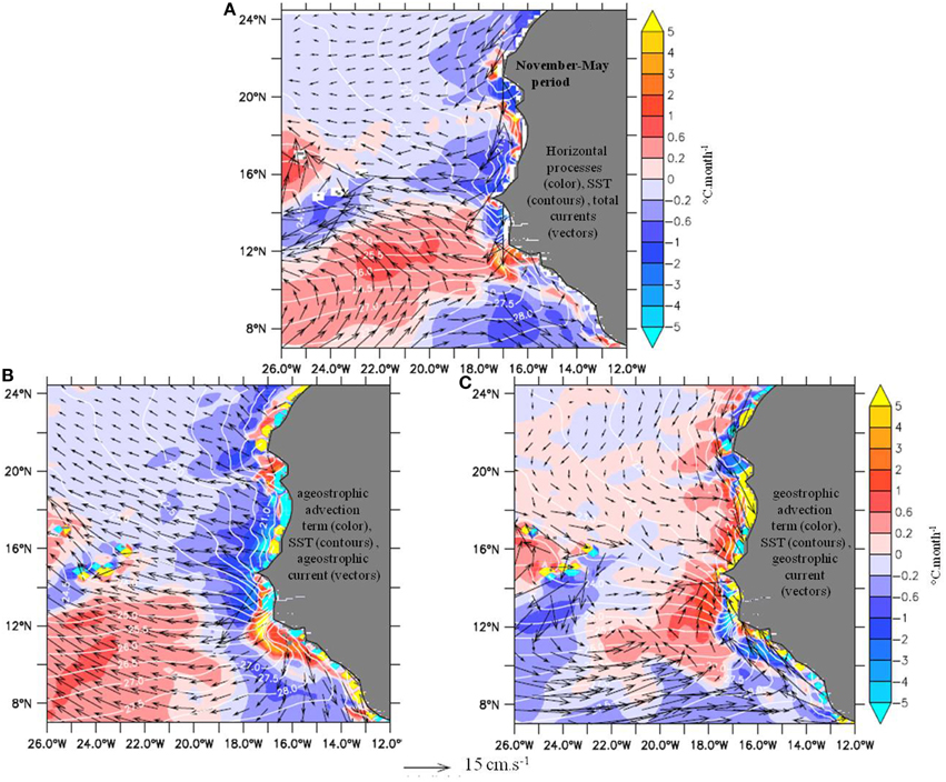
Figure 8. Horizontal processes effect in the model averaged over the CP. (A) Sum of horizontal advection and lateral diffusion (shading, °C.month−1), total currents (black vectors), (B) Ageostrophic advection term (shading, °C.month−1), ageostrophic currents (black vectors), and (C) geostrophic advection term (shading, °C.month−1), geostrophic currents (black vectors), and SST (white contours).
Along African coasts, each advective contribution dominates alternatively the total in function of latitude. North of about 17°N, the intense CJ, southward and geostrophic, dominates almost always the total effect. It advects upwelled waters and spread the cooling, particularly north of Cape Timiris (~19.5°N). Interestingly, there within 100–200 km from the shore, the cross-shore component of the SST gradient is sometime reversed with warmer waters inshore, which explains the warming effect of the north-westward Ekman drift. To the south however, until the Cape Verde Peninsula, the CJ cross-shore component is sometimes eastwards and warms the coast, through advection of offshore waters. Hence along south Mauritania and northern Senegal from 20 to 15°N, the CJ is not systematically causing cooling, which instead results from the ageotrophic flow. From 15 to about 12.5°N, the balance is comparable to north of Cape Timiris. There is a net cooling effect explained essentially by the CJ. At 12°N, one remarks the Senegal-Mauritania meridional front [42], maintained by the upwelling and the CJ to the north, and the intense geostrophic poleward SLJ to the south, which transports warm water alongshore. South of 12°N, both the SLJ and the southward Ekman currents are flowing in large part along homogeneous warm SST, and become thus less important for the SST change.
Farther offshore, west of about 18°W, and on regional scales, the SST shows weaker fronts, and advection is hence less intense. North of the CVA in particular, weak SST gradients explain the weak effect of advection. To the contrary, around the CVA and south of about 15°N, the advection pattern explains in large part the net ocean contribution, with intensities generally larger than those of vertical processes. In particular, the maximum net cooling visible at latitudes 12–16°N appears to be due, to the east, to westward advection of coastal waters by Ekman drift (Figure 8B) and, to the west, to southward advection by the Guinea gyre geostrophic circulation (Figure 8C). Finally, to the south of ~12°N, the warming longitudinal band is due to geostrophic MC and Ekman drift poleward transports, whereas the cooling pattern to the south-east is explained by the equatorward component of the NECC and the Ekman currents.
To complete the study of horizontal processes, it is worth saying that the diffusion term is significant nearshore with an intensity reaching locally up to ~1°C.month−1 between 10 and 19°N (not shown). Lateral temperature gradients and mesoscale eddies are stronger there. The warming tendency is consistent with the current understanding of the role of mesoscale turbulence [43] and with its manifestations in upwelling systems [44, 45]. Given our limited horizontal resolution, it is largely through lateral diffusion that these processes manifest themselves.
Now we proceed to the examination of the air-sea heat flux contribution (Figure 9A). Its structure is comparable to its annual mean (e.g., opposite to Figure 6A), except for a large domain of negative values, instead of positive, to the north-west of about (12°N, 19°W), and higher values along Mauritania and Morocco, as noted for all previous terms. The general structure is hence a coastal maximum, a rapid decrease until near 18°W where the sign changes, and a moderate decrease westward. Such a distribution is evidently due to that of the net heat flux (Figure 9B). The comparison of the radiative and turbulent components (Figures 9B,C) highlights that the second explains most of the pattern, since it varies zonally much more than the solar heat flux. Such variations east of about 18°W are explained in large part by the SST distribution. Close to the continent indeed, latent heat flux patterns are comparable to those of SST, due to a strong modulation of surface specific humidity. Similarly one observes minimum heat loss over cold coastal waters, north of the Senegal-Mauritania front (~12°N), and larger loss over the warm SLJ to the south nearshore (Figure 9C). The large-scale tilt in the distribution of the trade winds speed explains the more regular decrease of the net heat flux west of about 18°W. At last it is important to note that the zonal decrease of the air-sea flux contribution between the continent and about 18°W is in large part also explained by the sharp increase of the MLD (see Figure 7B) since it is in the denominator of term D in Equation (1). In conclusion, in the vicinity of the continent east of ~18°W, it is mainly SST and MLD structures, associated with coastal upwelling dynamics, which explain the intense damping of the oceanic processes by the air-sea fluxes. West of ~18°W, the westward increase of the trade winds speed explains the progressive passage to a more classical winter cooling regime by air-sea fluxes, to the exception of the CVA where local wind reduction in the lee of islands generates a net heat gain by the ocean.
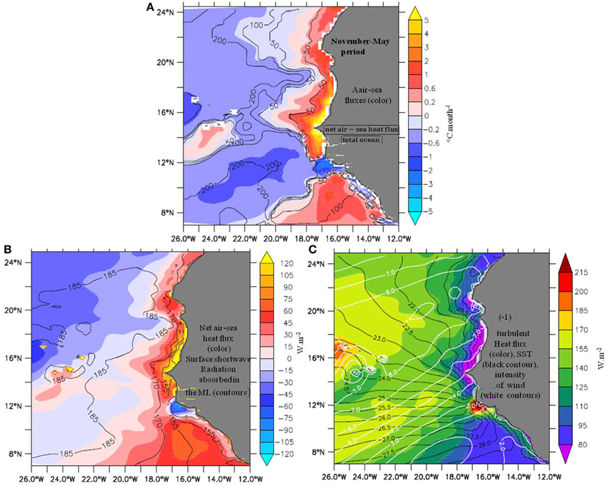
Figure 9. Contribution of air-sea heat fluxes to the ML heat budget over the CP. (A) trend associated with the net air-sea heat flux (shading,°C.month−1) and ratio of net air-sea heat fluxes effect over total ocean effect (black contours), (B) net air-sea heat flux (shading, W.m−2) and surface shortwave radiation absorbed in the ML (black contours), (C) turbulent heat fluxes (latent+sensible) (shading, W.m−2), SST (black contours, °C) and intensity of wind stress (white contours, N.m−2). The sign of latent heat flux (< 0) has been changed.
Overall, the comparison between ocean and air-sea fluxes contributions (see ratio of both contributions on Figure 9A) confirms that there are two main regimes for the region. East of 18°W, the ocean processes associated with coastal upwelling dynamics dominate the time-average cooling, whereas the air-sea fluxes damps it. West of this longitude band, the same opposition holds within the 12–18°N latitude band only, where the maximal net SST cooling centered at (16°N, 18°W) (Figure 3B) is due mainly to Ekman drift of cold coastal waters. North and south however, the air-sea fluxes dominate the ocean processes by at least a factor two. Note though that since the periods for time-averages were chosen to emphasize coherence in upwelling dynamics, ocean effect appears relatively intense. The net-air-sea flux in fact changes sign during CP, but explains month-to-month SST variations in large parts of the region, as we will see in Section The Sub-domain Next to the Continent.
June–October Warming Period
This period corresponds in time-average to a warming of the domain. The northward migration of the ITCZ causes a decrease of the coastal Ekman pumping south of 18°N, and an increase north of it (Figure 2). During WP, the contribution of the net air-sea heat flux is dominant over most of the domain as we will see, and we begin the analysis with it.
Figure 10 displays its time-mean contribution, and components. Overall the distribution resembles its annual mean. Compared to the CP mean, the structures of all quantities still display a rapid zonal variation of intensity from the coastline to about 18°W. Contrasts in longitude are weaker between 12 and 18°N, as expected from the lesser intensity of coastal dynamics associated with weaker Ekman pumping there. North of 15°N the air-sea flux effect decreases westward, first rapidly by a factor of ~2 and then smoothly by ~2 again (Figure 10A). It is due to the net air-sea flux distribution (Figure 10B), and also to the MLD westward increase (Figure 3D), both of them explaining the zonal change in roughly equal proportion. The net air-sea flux decrease arises from its turbulent component only, since solar radiation absorbed in the ML increases slightly westward (contours in Figure 10B). The turbulent heat loss is indeed rising to the west, due in main part, to SST distributions shaped by ocean circulation, in particular coastal dynamics associated with weak Ekman pumping (Figure 2). In the 15–20°N latitude band, it is also due to the wind speed increase to the west. To the north the wind speed decreases westward and effect on turbulent cooling is dominated by the SST increase. This result is consistent with the analysis by Foltz et al. [22] that also invokes the control by air-sea humidity gradients north of 20°N.
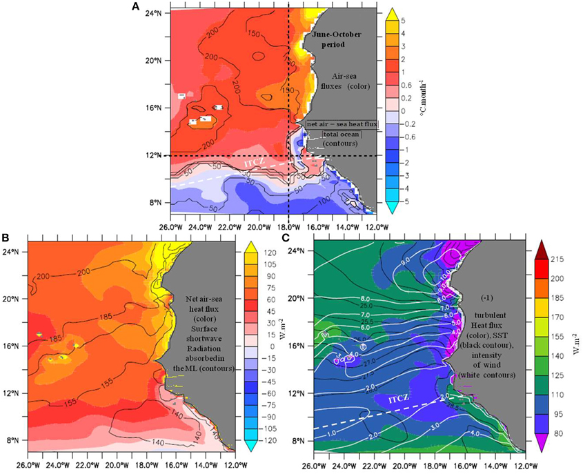
Figure 10. Same as in Figure 9 but over WP (June–October).
Regarding the abrupt meridional decrease of the net air-sea flux contribution in the south, it results from the combination of minimum incoming shortwave radiation (not shown) associated with the ITCZ cloud cover, and intensifying turbulent cooling due to equator-ward acceleration of the southern trade wind south of the ITCZ (white contours in Figure 10C). However the net air-sea flux is positive almost everywhere, and the net cooling contribution to the ML heat budget visible south of the ITCZ diagonal (Figure 10A) can only be due to the fraction of the solar flux that penetrates below the ML. This process will be confirmed by the examination of vertical processes contribution.
To conclude, it is worth noting the predominance in the net SST warming of the air-sea fluxes over the ocean processes north of the ITCZ region, whereas south of it, the weak SST variations are rather dominated by the ocean contribution.
Now we turn to the ocean contribution shown in Figure 11A. Its general structure is comparable to the annual mean, but for larger intensities to the north and south of the domain. The comparison with the contribution of vertical processes (Figure 11B) is striking and indicates that it explains most of the ocean contribution pattern. The ratio with the contribution of horizontal processes (contours in Figure 11A) shows however that north and south of the domain, horizontal processes are comparable contributors in terms of intensity. As during CP, the vertical processes contribution is dominated by far by vertical diffusion (not shown), but there are significant changes to this term compared to CP. First a domain scale latitudinal dipole appears on both sides of the ITCZ diagonal, and second the open-ocean diffusive cooling develops northward and westward, forming a relative maxima centered at (17°N, 19°W) (Figure 11B). Off-line reconstruction of the vertical diffusion effect indicates that is in large part explained by the vertical temperature gradient at the ML base, rather than by the vertical diffusion coefficient Kz (Figures 11C,D), except for the intensified Morocco upwelling. It is hence different than during CP. Kz is more homogeneous zonally and exhibits higher values far from the continent, possibly due to the weaker stratification at this period that is favorable to turbulence. Therefore the latitudinal variations of vertical stratification at the ML base become determining (Figure 11D), despite smaller values during this warming season. This relative weakness may seem surprising considering the intense seasonal surface warming, but during WP, a significant fraction of the solar radiation penetrates below the thin ML, and contributes to shaping smooth vertical profiles of temperature.
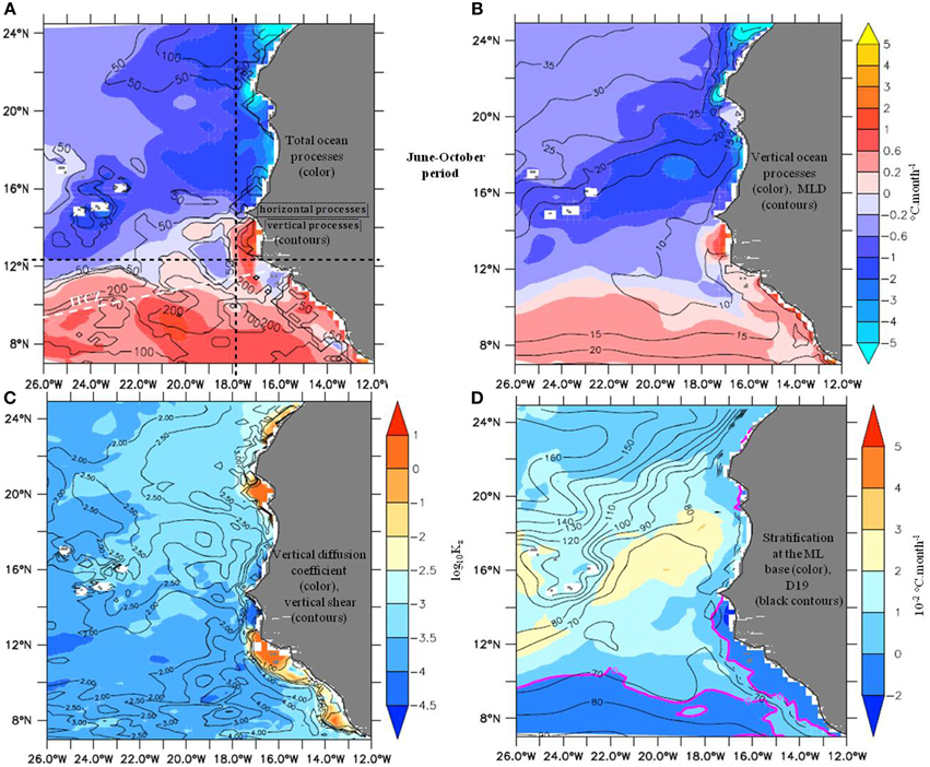
Figure 11. Same as in Figure 7 but over WP (June–October).
To explain the meridional structure of the subsurface stratification, it is first necessary to recall that the seasonal shift of the ITCZ is responsible of a northward shift of the open-ocean upwelling, which in turn lifts the thermocline (Figure 4D) and tends to enhance stratification north of about 15°N. Moreover, the ITCZ rainfall gives rise to barrier-layers, and associated temperature inversions at the ML base (Figure 11D) [41]. Consequently, vertical turbulence warms SST there. Looking at the diffusive warming and inversions distribution, it appears that it results from a combination of the large scale barrier layer distribution associated with the ITCZ and NECC [41], and from a narrow coastal band reaching further north up to the Cape Verde Peninsula, likely due to advection of equatorial fresh waters by the SLJ as well as local seasonal rainfall. Note that in line with other coastal modifications between CP and WP described above, large horizontal diffusion effects are displaced northward offshore Mauritania and Morocco coasts (not shown). Their intensities reach up to 0.6°C.month−1, corresponding to mesoscale eddy activities accompanying coastal upwelling.
During WP, horizontal advection still plays a significant role in the evolution of the SST, except for the zonal band located between 17 and 20°N. There it represents less than a quarter of the vertical oceanic processes (Figure 11A) due to currents largely parallel to the isotherms. Near-shore to the north of the domain, the cooling is essentially due to Ekman drift that follows the ITCZ migration (Figures 12A,B). It is shifted northward with a marked extreme and a large cross-shore extension north of 21°N. Around this latitude, warming occurs just at the coast because upwelling and SST minima are found at some distance offshore, as observed by Barton et al. [46], due to the wide plateau which affects structure and intensity of the upwelling. Interestingly, from Cape Timiris to the Cape Verde Peninsula within 100-300 km from the shore off Senegal and Mauritania, the imbalance between Ekman cooling and geostrophic warming by the MC (Figure 12C), is in favor of Ekman flow. This ageostrophic cooling reinforces the vertical processes cooling from the coastal upwelling (Figures 11B, 12A,B). Hence the simulation suggests that the WP time-mean net current contribution is dominated by the MC warming effect only far off-shore, west of 18°W. To the opposite, just south of Cape Verde Peninsula, the advection of warm waters brought by the MC dominates the Ekman drift, which leads to net warming by advection (Figures 12A–C). On the continental shelf south of 12°N, a coastal SST maximum leads to the same type of compensation between geostrophic currents (cooling) and Ekman drift (warming), described above for southern Morocco, with overall a weak advective effect on SST. West of 18°W, the modulation of the advective effects associated with the Cape Verde islands is unchanged relative to CP (Figures 8A, 12A). South of 12°N, the net warming by advection is due to the generally constructive contributions of Ekman and geostrophic (NECC) flows. Despite the high resulting velocities, the warming tendency remains modest because the temperature gradient in the area is weak.
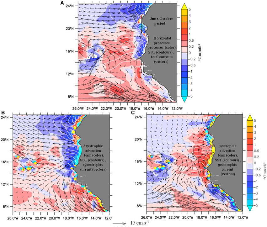
Figure 12. Same as in Figure 8 but over WP (June–October).
Considering the insights provided by the above spatial analysis, a finer understanding of the leads and lags between processes of the heat budget can be obtained by latitude-time diagrams of the zonally averaged terms. In the following, we present one diagram for each sub-domain, first for the continental zone east of 18°W, and second for the open-ocean area to the west. We focus on time transitions between heat budget regimes. Note that averaging coastal data over a varying distance corresponding to the plateau width offers similar results.
The Sub-domain Next to the Continent
Two latitudinal sectors emerge from Figure 13A. North of 12°N the SST experiences an annual cycle, whereas to the south it is semi-annual and forced by the two passages of the ITCZ (Figure 13A). As seen before, the strongest SST variations (>2°C.month−1) occur approximately from 12° to 20°N. At first sight the overall variations are in good phase with the net air-sea flux contribution (Figure 13B). We first study the cooling phases, which start early September north of the Cape Verde Peninsula, and later on further south (until December). North of ~20°N, the SST cooling phase is driven by the decrease of the net air-sea flux, warming effect, that become smaller than the cooling by upwelling dynamics. It is obviously due to the seasonal attenuation of solar radiations. The relative high intensity of the cooling effect by ocean processes is essential to the heat budget evidently, but not for its change from a net positive to net negative trend. It is not a driver since it entered a decreasing phase around this period, explained by the attenuation of the trade winds (Figure 4) and associated Ekman pumping (Figure 2). From ~20°N to the Cape Verde Peninsula (15°N), to the contrary the cooling effect by ocean processes strongly increases from early September to mid-October (from about −1 to ~ −2.5°C.month−1, Figure 13C), due to intensification of vertical turbulent mixing and along-shore southward advection, generated by the strengthening of the winds (Figures 2, 4, 13D,E). Note that horizontal processes, largely dominated by advection, have a cooling effect generally more than half as intense as the vertical processes (contours in Figure 13E). During this period, the warming effect by air-sea fluxes decreases in smaller proportions (from about 1 to ~0.5°C.month−1), thereby contributing slightly to the net cooling. The SST cooling peak in October is therefore explained by the constructive effects of both family of processes, dominated by the upwelling dynamics. From November to February, essentially the upwelling dynamics maintain the cooling rate. South of 15°N, it is clear that net air-sea flux again controls the early months of the cooling season. There, seasonal temperature inversion effects (Figure 13D) as well as northward advection of warm waters by the MC and SLJ (Figure 13E) warm the SST to the contrary.
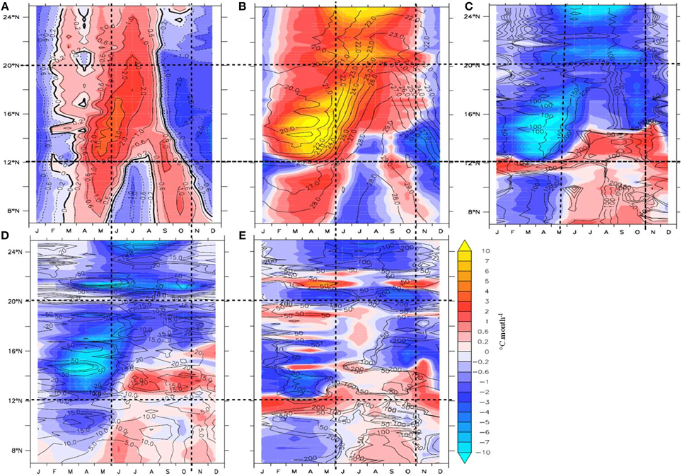
Figure 13. Latitude-time Hovmöller plots along the coastal region (averaged from the coast to 18°W) of the mean seasonal cycles. (A) model total temperature trend (shading and contours, °C.month−1), (B) air-sea heat vertical process (shading), and SST model (contours, °C), (C) total oceanic trend (shading, °C.month−1) and ratio of net air-sea flux effect over ocean effect (contours, %), (D) trend associated with vertical processes (shading, °C.month−1) and maximum vertical velocities between surface and thermocline (contours, m.month−1) and (E) horizontal processes (shading, °C.month−1) and ratio of horizontal processes over vertical processes (contours, %).
The second period of particular interest is the period when SST has reached minimum annual values, and starts to increase again, in March-April at all latitudes. It is almost everywhere a period of cooling by oceanic processes, especially intense south of Cape Timilis (~20°N) where Ekman pumping and upwelling velocities increase (Figure 2 and contours in Figure 13D). Vertical turbulent processes dominate the cooling (see ratio in contours, Figure 13C), whereas coastal horizontal currents favor or oppose them depending on latitude, as discussed in previous sections. The only exception is over the Senegal-Mauritania front (11-12°N), where the SST warming appears to be due primarily to the poleward advection of warm waters along-shore by the SLJ and off-shore spreading by the Ekman drift. Nevertheless, it is overall the seasonal increase of the net air-sea flux that sets the start of the warming season, whereas ocean processes act to reduce or delay the warming.
The Open Ocean
We now focus on the area west of 18°W. The SST temporal changes are broadly similar to those next to the continent, but share a much stronger resemblance with the net air-sea flux term (Figures 14A,B). In more details, the air-sea fluxes contribution displays everywhere the same pattern as the SST change. It is more intense most of the time, though, since the oceanic processes oppose it quasi systematically (Figures 14B,C). Two regions of exception deserve attention: north of ~18°N when the oceanic processes contribute weakly to the forcing of the SST decrease by the air-sea fluxes (October–February), and south of 10°N in September-October when the ocean forces mainly the second semi-annual warming. Overall, air-sea fluxes set the positive and negative trends in SST over most of the domain. Interestingly the ocean counter-action is not a mere passive damping. Indeed during WP, wind-driven vertical currents (contours in Figure 14D) amplify stratification and turbulent cooling, especially near 16°N as discussed in Figure 11. To the south, temperature inversions associated with ITCZ barrier layers restore to the surface the heat from solar radiations that penetrate below the ML (see especially Figure 11D). From 8 to 10°N they oppose the July cooling, but set the following warming. Additionally throughout the year horizontal advection, discussed in previous sections, also contribute to oppose the net air-sea flux effect (Figure 14E). Considering the spatial distributions analyzed previously, these results, derived in average, are more representative of the western part of the sub-domain. Indeed, closer to the continent and the islands, oceanic effects have larger amplitudes relative to the net air-sea flux (see Figures 9, 10). Also recall that the CP time-average had shown a positive mean contribution of the air-sea fluxes during the net SST cooling. This apparent contradiction, is due to the consistency of the sign of the ocean processes term over CP (negative during 4 out 6 months) relative to that of the net air-sea flux effect during the same period (half time negative, half time positive). Nevertheless, the main sign changes of the SST trend, in March and in September-October are driven by the net air-sea flux effect.
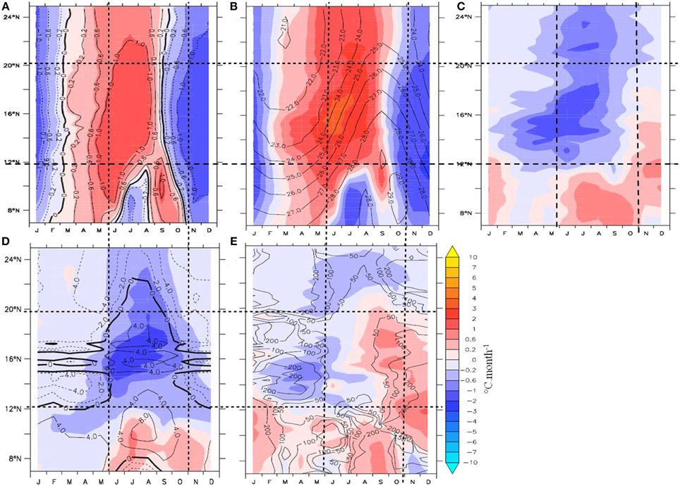
Figure 14. Same as in Figure 13 but for the heat budget terms averaged between18°W and 26°W.
Summary and Discussions
In this study, the seasonal cycle of the SST in the Atlantic North-eastern Tropical Upwelling System (ANETUS) is examined using a ML heat budget, in a numerical simulation of the Tropical Atlantic. The ANETUS domain is characterized by the presence of the continent to the east, the Guinea upwelling gyre and Guinea Dome, and the presence of the ITCZ. The contribution of the ocean processes to the heat budget is the focus of our study, and particularly the heat fluxes at the base of the ML that is difficult to compute from existing observations. Two main heat budget regimes emerge in annual mean on both sides of schematically latitude 12°N (related to the mean ITCZ location) and are quite representative of the time-varying contribution of ocean processes. Roughly, to the north, the mean regime is characterized by a tendency to cool the ML by ocean processes, generally dominated by vertical turbulent mixing intensified by Ekman pumping. To the south, the ocean processes tend generally to warm the surface, through advection by NECC, MC or SLJ and temperature inversions, and against a time-mean cooling by air-sea fluxes. The seasonal variations of the SST can be described by a CP of decreasing and then minimum SST (November-May), and a WP (June–October) of increasing SST reaching a maximum in summer. Both are, respectively, associated with maximum then minimum coastal upwelling south of ~20°N (Cape Timilis), and vice-versa north of the Cape. Two sub-domains in terms of ocean circulation and heat budget are separated grossly by longitude 18°W: a narrow continental band of a few degrees of longitude next to West-Africa characterized by ocean frontal dynamics and intense signals, and a vast open ocean region to the west that displays smoother fields and weaker signals. The seasonal heat budget explaining the SST cycle is:
(1) The continental band: the cooling starts early September north of the Cape Verde Peninsula. North of Cape Timilis, it is driven by the decrease of the net air-sea flux warming effect, due to the seasonal attenuation of solar radiation. It is damped by the decrease of the upwelling-forced cooling trend, due to the seasonal Ekman pumping attenuation. South of 20°N, down to the Cape Verde Peninsula (15°N), the constructive effects of both air-sea fluxes and, in larger proportion, upwelling dynamics, explain the SST cooling and its October peak of intensity. Later on the latter dominates the cooling season. From 15 to 7°N and from October to December, the net air-sea flux negative trend triggers the cooling, whereas temperature inversion and warm geostrophic currents damp it. Regarding the second phase of the SST cycle, the start of the warming season, regardless of latitude, is forced by the net air-sea flux, and damped by upwelling dynamics.
(2) The open ocean: The cooling and warming phases are fundamentally driven by the seasonal net air-sea flux effect, against the oceanic processes that partly oppose it, except north of 18°N particularly. The March SST cooling is slightly amplified by the intensifying Guinea Gyre upwelling in summer-autumn, which tends to cool the surface by turbulent mixing, especially near 16°N. Further south, warming by temperature inversions and horizontal currents, opposes the net air-sea flux effect.
Near the continent, our results support the preliminary model study by Carton and Zhou [20] pointing out to the leading role of wind-driven coastal upwelling dynamics for the SST cycle from 10 to 20°N. It is however verified only for the cooling phase from September to early March. The warming phase starting in March-April in our simulation is driven instead by the seasonal increase of the solar radiations. The detailed analysis of the upwelling dynamics suggests that the total horizontal contribution represents more than 50% of the effect associated with vertical processes in general. North of 20°N and south of 12°N, it is often stronger than the effect of vertical processes. Advection of waters, especially from the north, is therefore an essential contributor to the coastal upwelling system heat budget, when SST is in its decreasing phase. Over the open ocean, west of ~18°W, our result supports most of those of Foltz et al. [22]. South of the mean ITCZ location however, we could evidence warming by vertical turbulent processes associated with temperature inversions, found within barrier layers in the region. Due to these inversions, we found that the Guinea Dome upwelling is able to generate a surface cooling only in the northern half of the GD area. It clarifies the results from Yamagata and Iizuka [7], pertaining to the thermocline and not to the ML, which explained the decrease in heat content by horizontal and vertical divergence of the heat transport in all GD.
Our model results are limited by inherent errors due to the relatively low horizontal and vertical resolution near the coast, and uncertainties in air-sea fluxes. Despite the biases in the represented thermocline, ML and mesoscale structures, we hope that our paper can provide nevertheless a relevant basis for further studies of the variability of SST and currents in the ANETUS, in particular at other challenging time-scales, like intra-seasonal and interannual ones.
Important limitations in the present study are due to the scarcity of in-situ observations. Additional studies of ocean currents, upper ocean turbulence and mixing, and more robust estimates of air-sea heat fluxes are needed offshore West Africa. This will require the implementation of measuring instruments to monitor the coastal region over long time periods, such as fixed moorings performing oceanic and atmospheric measurements. Such measurements will allow us to better evaluate numerical models and improve our understanding of regional ocean-atmosphere exchanges and climate variability.
Conflict of Interest Statement
The Reviewer Vincent Michel Echevin declares that, despite having collaborated with the author Saliou Faye, and sharing an affiliation with the author Bamol A. Sow the review process was handled objectively. The authors declare that the research was conducted in the absence of any commercial or financial relationships that could be construed as a potential conflict of interest.
Acknowledgments
The research leading to these results has received funding from Centre de Recherche Océanographique Dakar-Thiaroye (CRODT/ISRA), Dakar-Sénégal and the International Joint Laboratory LMI ECLAIRS, as well as from the EU FP7/2007-2013 under grant agreement no. 603521. We thank B. Diaw, C. Ndour, H. Diadhiou, M. Fall, and Patrice Brehmer for their essential support throughout this study, and X. Capet. We are grateful to the anonymous reviewers for his helpful comments.
References
2. Chang P, Yamagata T, Schopf P, Behera SK, Carton J, Kessler WS, et al. Climate fluctuations of tropical coupled systems: the role of ocean dynamics. J Clim. (2006) 19:5122–74. doi: 10.1175/JCLI3903.1
3. Lathuilière C, Echevin V, Lévy M. Seasonal and intraseasonal surface chlorophyll-a variability along the northwest African coast. J Geophys Res. (2008) 113:C05007. doi: 10.1029/2007jc004433
4. Siedler G, Zangenberg N, Onken R, Molie‘re A. Seasonal changes in the tropical Atlantic circulation: observation and simulation of the Guinea Dome. J Geophys Res. (1992) 97:703–15. doi: 10.1029/91JC02501
5. Lazar A, Inui T, Malanotte-Rizzoli P, Busalacchi AJ, Wang L, Murtugudde R. Seasonality of the ventilation of the tropical Atlantic thermocline. J Geophys Res. (2002) 107:3104. doi: 10.1029/2000JC000667
6. Jiang H, Huang RX, Wang H. Role of gyration in the oceanic general circulation: Atlantic Ocean. J Geophys Res. (2008) 113:C03014. doi: 10.1029/2007jc004134
7. Yamagata T, Iizuka S. Simulation of the tropical thermal domes in the Atlantic: a seasonal cycle. J Phys Oceanogr. (1995) 25:2129–40.
8. Wooster, W, Bakun A, and McLain D. The seasonal upwelling cycle along the eastern boundary of the north Atlantic. J Mar Res. (1976) 34:131–41.
9. Allen JS. Upwelling and coastal jets in a continuously stratified ocean, J. Phys Oceanogr. (1973) 3:245–57.
10. Hagen E. Mesoscale upwelling variations off the West African coast. In: Richardson FA, editor. Coastal and Estuarine Sciences, Vol. I, Coastal Upwelling. Washington, DC: AGU (1981). pp. 72–8. doi: 10.1029/co001p0072
11. Hagen E. Northwest Africa upwelling scenario. Oceanol Acta (2001) 24(Suppl. 1):113–28. doi: 10.1016/S0399-1784(00)01110-5
12. Mason E, Colas F, Molemaker J, Shchepetkin AF, Troupin C, Sangrà P, et al. Seasonal variability of the Canary current: a numerical study. J Geophys Res. (2011) 116:C06001. doi: 10.1029/2010jc006665
13. Mittelstaedt E. The ocean boundary along the northwest African coast: circulation and oceanographic properties at the sea surface. Prog Oceanogr. (1991) 26:307–55. doi: 10.1016/0079-6611(91)90011-A
14. Stramma L, Huttl S, Schafstall, J. Water masses and currents in the upper tropical northeast Atlantic off northwest Africa. J Geophys Res. (2005) 110:C12006. doi: 10.1029/2005JC002939
15. Lazaro C, Fernandes-Santos M, Oliveira P. Seasonal and interannual variability of surface circulation in the Cape Verde region from 8 years of merged t/p and ers-2 altimeter data. Rem Sens Environ. (2005) 98:45–62. doi: 10.1016/j.rse.2005.06.005
16. Barton ED. Eastern boundary of the North Atlantic : Northwest Africa and Iberia. In: Robinson AR, Brink K, editors. In The Sea, Vol. 11. New York, NY: John Wiley and Sons, Inc. (1998). p. 633–57.
17. Mazeika PA. Thermal domes in the eastern tropical Atlantic Ocean. Limnol Oceanogr. (1967) 12:537–9. doi: 10.4319/lo.1967.12.3.0537
18. Doi T, Tomoki T, Toshio Y. Interannual variability of the Guinea Dome and its possible link with the Atlantic Meridional Mode. Clim Dyn. (2009) 33:985–98. doi: 10.1007/s00382-009-0574-z
19. Doi T, Tomoki T, Toshio Y. The Atlantic Meridional Mode and its coupled variability with the Guinea Dome. J Clim. (2010) 23:455–75. doi: 10.1175/2009JCLI3198.1
20. Carton JA, Zhou ZX. Annual cycle of sea surface temperature in the tropical Atlantic Ocean. J Geophys Res. (1997) 102:27813–24. doi: 10.1029/97JC02197
21. Yu LS, Jin, XZ, Weller, RA. Role of net surface heat flux in seasonal variations of sea surface temperature in the tropical Atlantic Ocean. Clim J. (2006) 19:6153–69. doi: 10.1175/JCLI3970.1
22. Foltz G, Schmid C, Lumpkin R. Seasonal cycle of the mixed layer heat budget in the Northeastern Tropical Atlantic Ocean. J Clim. (2013) 26:8169–88. doi: 10.1175/JCLI-D-13-00037.1
23. Nykjaer L, van Camp L. Seasonal and interannual variability of coastal upwelling along northwest Africa and Portugal from 1981 to 1991. J Geophys Res. (1994) 99:14197–207. doi: 10.1029/94jc00814
24. Santos MP, Kazmin AS, Peliz A. Decadal changes in the Canary upwelling system as revealed by satellite observations: their impact on productivity. J Mar Res. (2005) 63:359–79. doi: 10.1357/0022240053693671
25. Bonjean F, Lagerloef GSE. Diagnostic model and analysis of the surface currents in the Tropical Pacific Ocean. J Phys Oceanogr. (2002) 32:2938–54. doi: 10.1175/1520-0485(2002)032<2938:DMAAOT>2.0.CO;2
26. de, Boyer Montégut C, Madec G, Fischer AS, Lazar A, Iudicone D. A global mixed layer depth climatology based on individual profiles. J Geophys Res. (2004) 109:C12003. doi: 10.1029/2004JC002378
28. Molines JM, Barnier B, Penduff T, Brodeau L, Treguier AM, Theetten S, et al. Definition of the Interannual Experiment orca025-g70, 1958 2004. Technical Report, Laboratire des Ecoulements Geophysiques et Industriels, CNRS UMR 5519, Grenoble (2007).
29. Brodeau L, Barnier B, Tréguier A, Penduff T, Gulev S. An ERA40-based atmospheric forcing for global ocean circulations models. Ocean Modell. (2010) 31:88–104. doi: 10.1016/j.ocemod.2009.10.005
30. Large W, Yeager S. Diurnal to Decadal Global Forcing for Ocean and Seaice Models: The Data Sets and Climatologies. Technical Report TN-460+STR. Boulder, CO: National Center for Atmospheric Research, Boulder (2004).
31. Zhang Y, Rossow WB, Lacis AA, Oinas V, Mishchenko MI. Calculation of radiative fluxes from the surface to top of atmosphere based on ISCCP and other global data sets: refinements of the radiative transfer model and the input data. J Geophys Res. (2004) 109:D19105. doi: 10.1029/2003JD004457
32. Vialard J, Delecluse P. An OGCM Study for the TOGA Decade. Part I: role of salinity in the physics of the Western Pacific fresh pool. J Phys Oceanogr. (1998) 28:1071–88
33. Peter A-C, Le Hénaff M, du Penhoat Y, Menkès C, Marin F, Vialard J, et al. A model study of the seasonal mixed layer heat budget in the equatorial Atlantic. J Geophys Res. (2007) 111:C06014. doi: 10.1029/2005JC003157
34. Jouanno J, Marin F, du Penhoat Y, Sheinbaum J, Molines J-M. Seasonal heat balance in the upper 100 m of the equatorial Atlantic Ocean. J Geophys Res. (2011) 116:C09003. doi: 10.1029/2010jc006912
35. Roy C. Fluctuation of wind and upwelling variability off the Senegalese coast. Oceanolo. Acta (1989) 12:361–9.
36. Ndoye S, Capet X, Estrade P, Sow, B, Dagorne D, Lazar A, et al. SST Patterns and Dynamics of the Southern Senegal-Gambia Upwelling Center. J Geophys Res. (2014) 119:8315–35. doi: 10.1002/2014JC010242
37. Chelton DB, Schlax MG, Freilich MH, Milliff RF. Satellite measurements reveal persistent small-scale features in ocean winds. Science (2004) 303:978–83. doi: 10.1126/science.1091901
38. Estrade P, Marchesiello P, de Verdiere AC, Roy C. Cross-shelf structure of coastal upwelling: a two-dimensional extension of Ekman's theory and a mechanism for inner shelf upwelling shut down. J Mar Res. (2008) 66:589–616. doi: 10.1357/002224008787536790
39. Austin JA, Lentz SJ. The inner shelf response to wind-driven upwelling and downwelling. J Phys Oceanogr. (2002) 32:2171–93. doi: 10.1175/1520-0485(2002)032<2171:TISRTW>2.0.CO;2
40. Centurioni LR, Ohlmann JC, Niiler PP. Permanent meanders in the California Current System. J Phys Oceanogr. (2008) 38:1690–710. doi: 10.1175/2008JPO3746.1
41. Mignot J, Lazar A, Lacarra, M. On the formation of barrier layers and associated vertical temperature inversions: a focus on the northwestern tropical. J Atlantic Geophys Res. (2012) 117:C02010. doi: 10.1029/2011jc007435
42. Diakhaté M., de Coetlogon, G., Lazar A., Gaye AT. Intra-seasonal SST variability within tropical Atlantic upwellings. Soumis à Q J R Meteorol Soc. (in press). doi: 10.1002/qj.2657
43. Gent PR, McWilliams JC. Isopycnal mixing in ocean circulation models. J Phys Oceanogr. (1990) 20, 150–5.
44. Capet X, Colas F, McWilliams JC, Penven P, and Marchesiello P. Eddies in eastern boundary subtropical upwelling systems. In: Hecht M, Hasumi H, editors. Ocean Modeling in an Eddying Regime. Geophysical Monograph Series, Vol. 177. Washington, DC: American Geophysical Union (2008). 131–48. doi: 10.1029/177GM10
45. Colas F, McWilliams JC, Capet X, and Kurian J. Heat balance and eddies in the Peru-Chile current system. Clim Dyn. (2012) 39:509–29. doi: 10.1007/s00382-011-1170-6
Keywords: SST, upwelling, circulation, heat budget, observations, modeling
Citation: Faye S, Lazar A, Sow BA and Gaye AT (2015) A model study of the seasonality of sea surface temperature and circulation in the Atlantic North-eastern Tropical Upwelling System. Front. Phys. 3:76. doi: 10.3389/fphy.2015.00076
Received: 28 February 2015; Accepted: 24 August 2015;
Published: 15 September 2015.
Edited by:
María Belén Rodríguez de Fonseca, Universidad Complutense de Madrid, SpainReviewed by:
Ana María Durán-Quesada, University of Costa Rica, Costa RicaTomoki Tozuka, University of Tokyo, Japan
Vincent Michel Echevin, Laboratoire d'Océanographie et du Climat: Expérimentations et Approches Numériques, France
Copyright © 2015 Faye, Lazar, Sow and Gaye. This is an open-access article distributed under the terms of the Creative Commons Attribution License (CC BY). The use, distribution or reproduction in other forums is permitted, provided the original author(s) or licensor are credited and that the original publication in this journal is cited, in accordance with accepted academic practice. No use, distribution or reproduction is permitted which does not comply with these terms.
*Correspondence: Saliou Faye, Laboratoire de Physique de l'Atmosphère et de l'Océan Simeon Fongung/École Supérieure Polytechnique/Université Cheikh Anta Diop, BP 5085 Dakar–Fann, Senegal;
Centre de Recherche Océanographique Dakar-Thiaroye (CRODT/ISRA), BP 2241 - Dakar, Senegal,c2FsaW91LmZheWVAdWNhZC5lZHUuc24=