 A. Arango-Restrepo
 J. M. Rubi
 Srutarshi Pradhan
- 1Departament de Física de La Matèria Condensada, Universitat de Barcelona, Barcelona, Spain
- 2Institut De Nanociencia I Nanotecnologia, Universitat De Barcelona, Barcelona, Spain
- 3PoreLab, Department of Physics, Norwegian University of Science and Technology, Trondheim, Norway
Fiber breakage process involves heat exchange with the medium and energy dissipation in the form of heat, sound, and light, among others. A purely mechanical treatment is therefore in general not enough to provide a complete description of the process. We have proposed a thermodynamic framework which allows us to identify new alarming signals before the breaking of the whole set of fibers. The occurrence of a maximum of the reversible heat, a minimum of the derivative of the dissipated energy, or a minimum in the stretching velocity as a function of the stretch can prevent us from an imminent breakage of the fibers which depends on the nature of the fiber material and on the load applied. The proposed conceptual framework can be used to analyze how dissipation and thermal fluctuations affect the stretching process of fibers in systems as diverse as single-molecules, textile and muscular fibers, and composite materials.
1 Introduction
When external load/stretch is applied on fiber materials composed of elements with different strength thresholds, weaker elements fail first. As the surviving elements have to support the load, stress (load per element) increases and that can trigger more element failure. With continuous loading/stretching, at some point the system collapses completely, that is, the external load/stretch is above the strength of the whole system at that point. Such a system collapse is known as “catastrophic failure” for that system.
There are several physics-based approaches [1–3] that can model such a scenario. Fiber bundle model (FBM) is one of those models, and FBM has become a useful tool for studying fracture and failure [4–6] of composite materials under different loading conditions. The simplicity of the model allows achieving analytic solutions [5, 7] to an extent that is not possible in any of the fracture models studied so far. For these reasons, FBM is widely used as a model of breakdown that extends beyond disordered solids. In fact, fiber bundle model was first introduced by a textile engineer [4]. Later, physicists took interest in it, mainly to explore the failure dynamics and avalanche phenomena in this model [8–10]. Furthermore, it has been used as a model for other geophysical phenomena, such as snow avalanche [11], landslides [12, 13], biological materials [14], or even earthquakes [15].
Although stretching processes in FBM have been analyzed extensively [1–6], mainly by the physics community, a concrete thermodynamic description for the stretching process is still lacking in this field. In the efforts to unveil the stretching failure phenomena, thermodynamics seems to be an important tool because it allows incorporating variables such as temperature, entropy, reversible heat, entropy production rate, and energy dissipation to thus unify stretching failure dynamics and energy analysis, especially where surface effects, heat release, and sound emission, due to energy dissipation, are present when dealing with the stretching failure of fibrous materials.
In this article, we intend to develop a thermodynamic framework to analyze not only the energetics of the stretching failure phenomena but also the dynamics by means of nonequilibrium thermodynamic formalism at all scales, from a single molecule to a macrostructure. We believe that our thermodynamic framework could carry over to other problem areas, eventually also outside the physical sciences such as molecular biology and nanotechnology.
We arrange the article as follows: After the Introduction (section 1), we give a short background of studies on stretching of FBM in section 2. In several subsections of section 2, we discuss strength and stability in FBM, energy variations during stretching, and warning signs of catastrophic failure. In section 3, we introduce a proper thermodynamic framework of the stretching process and analyze the mesoscopic regime and small-fluctuation regime. All the simulation results are presented in section 4, including dynamics and energetics, the Fokker–Plank approach, and the role of fluctuations on the stretching process. We make some conclusions at the end (section 5).
2 Background: Stretching of a Fiber Bundle
In 1926, F. T. Peirce introduced the fiber bundle model [4] to study the strength of cotton yarns in connection with textile engineering. Some static behavior of such a bundle (with equal load sharing by all the surviving fibers, following a failure) was discussed by Daniels in 1945 [16], and the model was brought to the attention of physicists in 1989 by Sornette [17].
In this model, a large number of parallel Hookean springs or fibers are clamped between two horizontal platforms; the upper one (rigid) helps hanging the bundle, while the load hangs from the lower one. The springs or fibers are assumed to have different breaking strengths. Once the load per fiber exceeds a fiber’s own threshold, it fails and cannot carry the load any more. The load/stress it carried is now transferred to the surviving fibers. If the lower platform deforms under loading, fibers closer to the just-failed fiber will absorb more of the load than those further away, and this is called the local load sharing (LLS) scheme [18]. On the other hand, if the lower platform is rigid, the load is equally distributed to all the surviving fibers. This is called the equal load sharing (ELS) scheme. Intermediate range load redistribution is also studied (see [19]).
2.1 Strength and Stability in a Fiber Bundle Model
Let us consider a fiber bundle model having N parallel fibers placed between two stiff bars (Figure 1). Under an external force, the system responds linearly with an elastic force. The dimensionless elastic force
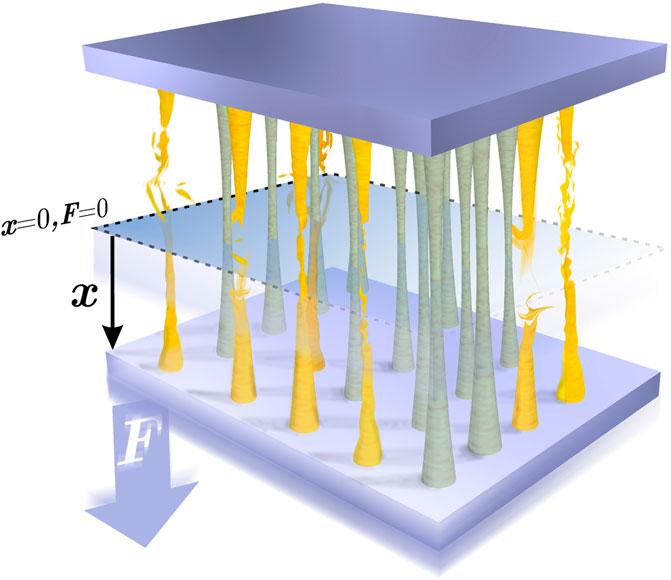
FIGURE 1. Illustration of the system. Under the application of a constant external force F, the set of fibres are stretched by a length x. As the fibers have different strength thresholds, some of them break (yellow fibres) resulting in the increment of load for the non-broken fibres (grey fibres).
2.1.1 Fiber Strength Distribution
The strength thresholds of the fibers are drawn from a probability density
from which we can obtain the number of non-broken fibers as a function of the average deformation of the set of fibers x:
The fraction of broken fibers, or damage, is then given by
2.1.2 The Critical/Failure Strength
The bundle exhibits an elastic force
The normalized elastic force
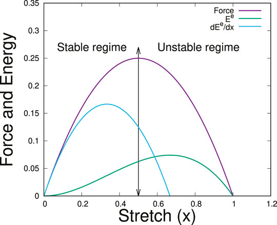
FIGURE 2. Force and energy against stretch x for a uniform distribution of the fiber strengths in the bundle, that is, for
The elastic force maximum is the strength of the bundle and the corresponding stretch value
The critical stretch value follows from the condition
2.2 Energies in Fiber Bundle Model During Stretching
When N is large, one can express the elastic
and
For a uniform distribution within the range
2.3 The Warning Signal of a Catastrophic Failure
The elastic energy reaches a maximum value which falls in the unstable region of Figure 2, after the critical value of the extension. Its knowledge is thus not useful to predict the catastrophic failure point of the system. However, the maximum value
The rate of change of the elastic energy thus shows a peak before the failure comes [20].
3 Thermodynamics of Stretching Processes
The stretching failure of fibers/materials is seen at a small scale, for example, during stretching of molecules in biological objects [21]. Similar stretching failure phenomena are also observed on a much bigger scale, like in the case of bridges made of long cables [22]. The observation in Ref. [20] that elastic energy variation could be a useful indicator of upcoming stretching-induced failure motivates us to construct a proper thermodynamic framework for such stretching failure phenomenon. For this purpose, we are going to introduce some new concepts like thermal bath, irreversible energy dissipation, and entropy production, and we believe that such a framework will help explore some new features of stretching failure behavior in general. In this section, we will compute the energy dissipated and the heat released in the stretching process and show that dissipation provides a warning signal of the failure.
3.1 Energetics
Due to the load F, the system experiences an external work W which affects the elastic and breaking energies and the entropy S as well. Energy conservation can thus be formulated as
where
where
The work done by the external force is the sum of the work done on each fiber:
where the work per fiber w is
Changes in the entropy in the stretching process are expressed as
where
where
where σ is the entropy production rate. The Goudy–Stodola theorem relates the total energy dissipated
At this point, it is important to distinguish between reversible heat
3.2 Mesoscopic Nonequilibrium Thermodynamics
When the fibers are immersed in a heat bath, their length can fluctuate. The effect of these fluctuations is negligible when the energy of the fibers is much greater than the thermal energy
The probability density
ensuing from probability conservation. In this equation, J is the probability current which vanishes at the boundaries (
By coupling linearly, the flux J and its conjugated thermodynamic force (chemical potential gradient
which corresponds to Fick’s diffusion law written in a dimensionless form where
with H being the enthalpy to which the elongation work and the elastic (potential) energy contribute. From now on, we will use the dimensionless force per fiber
For large values of f, the entropic contribution is very small. Notice that the signs of the enthalpic terms have been changed because the external work is done in the direction of the movement, while the elastic force has the opposite direction.
Substituting Eq. 20 in Eq. 18 and the resulting flux in Eq. 16, we obtain the Fokker–Planck equation describing the evolution of the probability distribution
The average elongation of the fibers corresponds to the first moment of the probability density ρ, and the solution of this equation is
Taking the time derivative of Eq. 22 and using the conservation law (Eq. 16), we obtain
from which we can interpret J as the local stretching velocity.
3.3 Small Fluctuation Regime
When fluctuations are very small, the variance of the probability distribution takes very small values, and therefore, we could approximate
where we have used the definition of φ. Integrating now Eq. 24 in x, we obtain the stretching velocity
where the first term on the right side is the entropic contribution, the second results from the presence of the load, and the third is due to the elastic force which opposes to the elongation of the fibers. For very small fluctuations, the entropy production rate Eq. 17 is
4 Results and Discussion
In this section, we obtain analytic expressions and numerical results for the dynamics and energetics of the stretching process assuming a uniform distribution of the strength thresholds of the fibers,
4.1 Dynamics and Energetics for Small Fluctuations
4.1.1 Dynamics
The average stretching velocity for a uniform distribution is obtained from Eq. 25, which is now written as
Its derivative with respect to the elongation given by
has a minimum around
For
4.1.2 Energetics
From the dynamic of the process, we can compute the work, the energies, and the heat involved. The work follows from Eqs. 10, 11:
The breaking energy, computed from Eq. 9, is
As expected, the breaking energy increases as the elongation increases. From Eq. 8, the elastic energy change is
and its derivative
From these expressions, we observe that the maximum of
On the other hand, the energy dissipated (Eq. 15) is
which decreases when κ increases because at a large elastic constant, more elastic energy can be stored to be subsequently transformed into kinetic energy after the breaking of the fibers. The first derivative of the energy dissipated, given by
must be positive, according to the second law which imposes that
Finally, the reversible heat
Its derivative with respect to the elongation
shows that the maximum of
From this expression, one can see that for
Another way to find alarming signals is to calculate the intersection point of the curves
For
4.2 Fokker–Planck Approach
To analyze the dynamic and the energetics of the process in the case in which fluctuations are not necessarily small, we will use the Fokker–Planck equation (Eq. 21) from which we can obtain the average elongation of the fibers and the energy dissipated. We have solved this equation by implementing the finite difference method in the software MATLAB 2017b. The results for ρ, represented in Figure 3, show a Gaussian-like behavior. We can observe that as the process progresses, the solution displaces to the right. In the inset, we represent the variance for
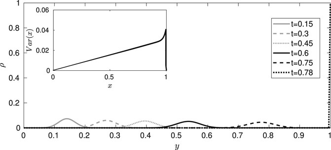
FIGURE 3. Probability density as a function of the elongation y at different times, for
By using Eqs. 2, 22, we compute the average elongation and the number of non-broken fibers which are represented in Figure 4. Both quantities exhibit a quasi-linear behavior and an asymptotic behavior close to the breaking point. This comes from the fact that by decreasing the number of non-broken fibers, the force exerted per fiber increases, thus triggering an accumulative effect, typical of catastrophic events. The inset of the figure shows a non-monotonic behavior of the damage rate, evidencing the competition between the elastic and external forces in the stretching process in which finally the load force per fiber becomes much higher and the rate increases exponentially.
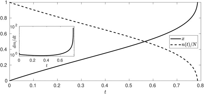
FIGURE 4. Average elongation of the set of fibers x (continuous line) and fraction of non-broken fibers n/N (dashed line) as a function of time t, for
The stretching velocity
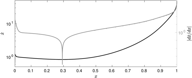
FIGURE 5. Stretching velocity
From the dynamics of the process, we can calculate the energy dissipated by using Eqs. 14, 15, 17. Figure 6 shows the energetics of the process. As predicted from the analytical results, we observe a maximum of the elastic energy and of the reversible heat. Furthermore, the maximum of
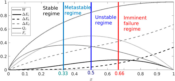
FIGURE 6. Energetics as the stretching progress, for
The derivatives of the different energies with respect to x are represented in Figure 7. Before the imminent failure regime, the behavior of the temporal derivatives coincides with that of the spatial derivatives due to the fact that in this regime, x is linear in time, as follows from Eq. 29. The results obtained confirm that the derivative of the elastic energy has a maximum at
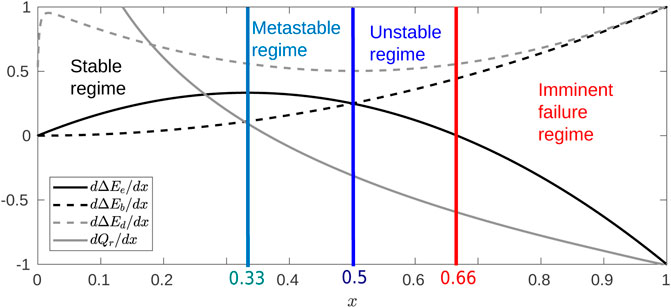
FIGURE 7. Derivatives for the energies of the stretching process as a function of the average elongation x, for
From Figure 7, we also confirm the fact that the derivative of the dissipated energy is always positive, in accordance with the second law of thermodynamics. Interestingly, the minimum of this derivative is found around
4.3 Role of the Fluctuations in the Stretching Process
The role that fluctuations play in the process can be estimated by comparing the value of the relevant quantities when we use the small fluctuation approach or when we adopt a Fokker–Planck description for the same value of κ. Figure 8 shows the change of the stretching velocity with position. In particular, for
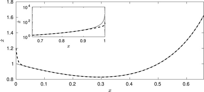
FIGURE 8. Results for the stretching velocity
As shown in Figure 9, energy dissipation and reversible heat are affected by fluctuations at all stages of the process. The dissipated energy is overestimated in the approach of small fluctuations, whereas the reversible net heat (
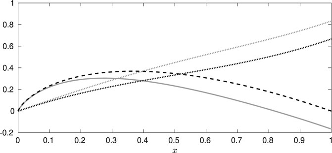
FIGURE 9. Dissipated energy and reversible heat as a function of the average elongation x, for
Figures 8, 9 show that the small fluctuation approach adequately describes the dynamics but not the energetics. The high accuracy in the dynamics is due to the almost Gaussian nature of the probability with a sufficiently small variance which is represented in Figure 3. The observed disparity in the reversible heat and energy dissipated lies in the approximation used. Additionally, the small deviation of the stretching velocity is accumulated, thus affecting the energy dissipated in the case of small fluctuation. Differences between both approaches become even more patent at smaller values of κ and f when the effect of the fluctuations is less important.
5 Conclusion
We have proposed a thermodynamic framework that analyses the role played by dissipation in a fiber stretching process, describes its different stages, and obtains new alarming signals before the whole set of fibers break. Our thermodynamic framework has identified relevant regimes (metastable, unstable, and imminent failure) as well as provided new transition indicators in terms of stretching velocity variation and entropy production rate, which is an important quantity to measure the energy efficiency of processes [27]. Specifically, we have shown that the maximum of the reversible heat may emerge before the process enters into the unstable regime. For some values of κ and small fluctuations, this maximum is located in the stable regime. In the same line, we found that the minimum of the entropy production rate is located around the transition to the unstable regime, and that for small fluctuations, this minimum defines the starting of the imminent failure regime for all values of κ. We have also proved that when the heat release flux is equal to the entropy production rate, in this intersection, the system is close to the transition toward the metastable regime. Similarly, we found that the minimum of the stretching velocity is always located in the stable zone, but the exact location strongly depends on the value of κ.
Under this approach, a more general analysis of the stretching process as a function of
Data Availability Statement
The raw data supporting the conclusions of this article will be made available by the authors, without undue reservation.
Author Contributions
AAR and JMR developed the idea, proposed the thermodynamic formalism used, and wrote the first version of the article. SP suggested the problem and supervised the results obtained. All authors contributed equally to the discussion of the manuscript.
Conflict of Interest
The authors declare that the research was conducted in the absence of any commercial or financial relationships that could be construed as a potential conflict of interest.
Acknowledgments
The authors are grateful to the Research Council of Norway for its Center of Excellence Funding Scheme, project no. 262644, and to PoreLab which partially funded the stay of JMR in Tronndheim. AAR and JMR acknowledge financial support of MICIU (Spanish government) under Grant No. PGC2018–098373-B-I00 and of the Catalan government under Grant 2017-SGR-884. AAR is grateful for the financial support through an APIF 2017–2018 scholarship from the University of Barcelona. We would like to thank Signe Kjelstrup, Dick Bedeaux, Alex Hansen, and in general the members of PoreLab for interesting discussions during the visit of two of us (JMR and AAR) to PoreLab.
References
1. Chakrabarti BK, Benguigui LG. Statistical Physics of Fracture and Breakdown in Disordered Systems. 55 Oxford and New York, NY: Oxford University Press (1997). 176 p.
2. Herrmann HJ, Roux S. Statistical Models for the Fracture of Disordered Media. North Holland: Elsevier (1990). 353 p.
3. Biswas S, Ray P, Chakrabarti BK. Statistical Physics of Fracture, Breakdown, and Earthquake: Effects of Disorder and Heterogeneity. Weinheim, Germany: John Wiley & Sons (2015). 344 p.
4. Peirce FT. Tensile Tests for Cotton Yarns: “The Weakest Link” Theorems on the Strength of Long and of Composite Specimens. J Textile Inst (1926) 17:T355–368. doi:10.1080/19447027.1926.10599953
5. Pradhan S, Hansen A, Chakrabarti BK. Failure Processes in Elastic Fiber Bundles. Rev Mod Phys (2010) 82:499–555. doi:10.1103/RevModPhys.82.499
6. Hansen A, Hemmer PC, Pradhan S. The Fiber Bundle Model: Modeling Failure in Materials. Weinheim, Germany: John Wiley & Sons (2015). 256 p.
7. Pradhan S, Chakrabarti BK. Precursors of Catastrophe in the Bak-Tang-Wiesenfeld, Manna, and Random-Fiber-Bundle Models of Failure. Phys Rev E (2001) 65:016113. doi:10.1103/PhysRevE.65.016113
8. Hemmer PC, Hansen A. The Distribution of Simultaneous Fiber Failures in Fiber Bundles. J Appl Mech (1992) 59:909–14. doi:10.1115/1.2894060
9. Pradhan S, Hansen A, Hemmer PC. Crossover Behavior in Burst Avalanches: Signature of Imminent Failure. Phys Rev Lett (2005) 95:125501. doi:10.1103/PhysRevLett.95.125501
10. Pradhan S, Hemmer PC. Relaxation Dynamics in Strained Fiber Bundles. Phys Rev E (2007) 75:056112. doi:10.1103/PhysRevE.75.056112
11. Reiweger I, Schweizer J, Dual J, Herrmann HJ. Modelling Snow Failure With a Fibre Bundle Model. J Glaciol (2009) 55:997–1002. doi:10.3189/002214309790794869
12. Cohen D, Lehmann P, Or D. Fiber Bundle Model for Multiscale Modeling of Hydromechanical Triggering of Shallow Landslides. Water Resour Res (2009) 45:W10436. doi:10.1029/2009WR007889
13. Pollen N, Simon A. Estimating the Mechanical Effects of Riparian Vegetation on Stream Bank Stability Using a Fiber Bundle Model. Water Resour Res (2005) 41:W07025. doi:10.1029/2004WR003801
14. Pugno NM, Bosia F, Abdalrahman T. Hierarchical Fiber Bundle Model to Investigate the Complex Architectures of Biological Materials. Phys Rev E (2012) 85:011903. doi:10.1103/PhysRevE.85.011903
15. Sornette D. Mean-Field Solution of a Block-Spring Model of Earthquakes. J Phys France (1992) 2:2089–96. doi:10.1051/jp1:1992269
16. Daniels HE, Jeffreys H. The Statistical Theory of the Strength of Bundles of Threads. I. Proc R Soc Lond Ser A. Math Phys Sci (1945) 183:405–35. doi:10.1098/rspa.1945.0011
17. Sornette D. Elasticity and Failure of a Set of Elements Loaded in Parallel. J Phys A: Math Gen (1989) 22:L243–50. doi:10.1088/0305-4470/22/6/010
18. Harlow DG, Phoenix SL. Approximations for the Strength Distribution and Size Effect in an Idealized Lattice Model of Material Breakdown. J Mech Phys Sol (1991) 39:173–200. doi:10.1016/0022-5096(91)90002-6
19. Hidalgo RC, Moreno Y, Kun F, Herrmann HJ. Fracture Model With Variable Range of Interaction. Phys Rev E (2002) 65:046148. doi:10.1103/PhysRevE.65.046148
20. Pradhan S, Kjellstadli JT, Hansen A. Variation of Elastic Energy Shows Reliable Signal of Upcoming Catastrophic Failure. Front Phys (2019) 7:106. doi:10.3389/fphy.2019.00106
21. Bering E, Kjelstrup S, Bedeaux D, Rubi JM, de Wijn AS. Entropy Production Beyond the Thermodynamic Limit From Single-Molecule Stretching Simulations. J Phys Chem B (2020) 124:8909–17. doi:10.1021/acs.jpcb.0c05963
22. Li D, Ou J, Lan C, Li H. Monitoring and Failure Analysis of Corroded Bridge Cables Under Fatigue Loading Using Acoustic Emission Sensors. Sensors (2012) 12:3901–15. doi:10.3390/s120403901
23. De Groot SR, Mazur P. Non-Equilibrium Thermodynamics. New York, NY: Courier Corporation (2013). 510 p.
24. Bejan A, Tsatsaronis G, Moran M. Thermal Design and Optimization. New York, NY: John Wiley & Sons (1996). 560 p.
25. Rubi JM, Bedeaux D, Kjelstrup S. Thermodynamics for Single-Molecule Stretching Experiments. J Phys Chem B (2006) 110:12733–7. doi:10.1021/jp061840o
26. Reguera D, Rubí JM, Vilar JMG. The Mesoscopic Dynamics of Thermodynamic Systems. J Phys Chem B (2005) 109:21502–15. doi:10.1021/jp052904i
27. Kjelstrup S, Bedeaux D, Johannessen E, Gross J. Non-Equilibrium Thermodynamics for Engineers. 2nd ed. World Scientific (2017). 510 p.
28. Roux S. Thermally Activated Breakdown in the Fiber-Bundle Model. Phys Rev E (2000) 62:6164–9. doi:10.1103/PhysRevE.62.6164
29. Pradhan S, Chakrabarti BK. Failure Due to Fatigue in Fiber Bundles and Solids. Phys Rev E (2003) 67:046124. doi:10.1103/PhysRevE.67.046124
Keywords: fiber bundle model, alarming signal, mesoscopic nonequilibrium thermodynamics, Fokker–Planck equation, dissipation, entropy production
Citation: Arango-Restrepo A, Rubi JM and Pradhan S (2021) A Thermodynamic Framework for Stretching Processes in Fiber Materials. Front. Phys. 9:642754. doi: 10.3389/fphy.2021.642754
Received: 16 December 2020; Accepted: 08 February 2021;
Published: 28 April 2021.
Edited by:
Antonio F. Miguel, University of Evora, PortugalReviewed by:
Antonio Heitor Reis, University of Evora, PortugalZhi Zeng, Hefei Institutes of Physical Science (CAS), China
Copyright © 2021 Arango-Restrepo, Rubi and Pradhan. This is an open-access article distributed under the terms of the Creative Commons Attribution License (CC BY). The use, distribution or reproduction in other forums is permitted, provided the original author(s) and the copyright owner(s) are credited and that the original publication in this journal is cited, in accordance with accepted academic practice. No use, distribution or reproduction is permitted which does not comply with these terms.
*Correspondence: Srutarshi Pradhan, c3J1dGFyc2hpLnByYWRoYW5AbnRudS5ubw==