 Ryutaro Mori
 Ruiyun Liu2
 Yu Chen
- 1Department of Social Psychology, Graduate School of Humanities and Sociology, The University of Tokyo, Hongo, Japan
- 2Department of Human and Engineered Environmental Studies, Graduate School of Frontier Science, The University of Tokyo, Kashiwa, Japan
Time irreversibility of a time series, which can be defined as the variance of properties under the time-reversal transformation, is a cardinal property of non-equilibrium systems and is associated with predictability in the study of financial time series. Recent pieces of literature have proposed the visibility-graph-based approaches that specifically refer to topological properties of the network mapped from a time series, with which one can quantify different degrees of time irreversibility within the sets of statistically time-asymmetric series. However, all these studies have inadequacies in capturing the time irreversibility of some important classes of time series. Here, we extend the visibility-graph-based method by introducing a degree vector associated with network nodes to represent the characteristic patterns of the index motion. The newly proposed method is parameter-free and temporally local. The validation to canonical synthetic time series, in the aspect of time (ir)reversibility, illustrates that our method can differentiate a non-Markovian additive random walk from an unbiased Markovian walk, as well as a GARCH time series from an unbiased multiplicative random walk. We further apply the method to the real-world financial time series and find that the price motions occasionally equip much higher time irreversibility than the calibrated GARCH model does.
Introduction
A time series with
Recently, the time (ir)reversibility of time series obtained in different domains have been investigated intensively because they provide rich information on the original dynamics themselves. For example, in the realm of physiology, it has been suggested that the time irreversibility in heartbeat weakens with aging or heart disease, and, therefore, a quantitative measurement of time (ir)reversibility may provide a way to assess the functionality of the biological system [8].
Among various application studies, the time irreversibility of financial time series attracts much interest from researchers for the following two reasons. First, it can help us to reveal the mechanisms of stylized facts concerned with the asymmetry of fluctuations in financial markets, specifically the gain–loss asymmetry and the leverage effect. Stylized facts of financial markets are a set of robust empirical patterns or properties that have been derived from data analytic studies across different financial markets or assets [9–11] such as fat-tailed distribution of returns [11–13], volatility clustering [11, 14–18], and the gain–loss asymmetry [10, 19]. A major research approach of financial markets is to build theoretical or numerical models that can reproduce stylized facts, and utilize the models to investigate their cause, or to predict the outcome of financial policies [11]. Hence, providing a novel tool for the investigation of their precise features or for the calibration of the models is of fundamental importance. The second reason is that one can estimate the predictability of financial index (e.g., stock price) from the time irreversibility of the series1. The connection between the time irreversibility and the predictability of financial time series is explained via the so-called efficient market hypothesis (EMH, in its weak form). The efficiency of a financial market here means that all the publicly available information is incorporated into the present market price; hence, a completely efficient market has no residual information available for predicting the future market prices. In turn, the existence of the predictability in financial time series requires a somewhat inefficiency of the market, which corresponds to the existence of extra information in the past sequence (i.e., memory). This existence of residual information implies that the time series should be sensitive to the direction of time (i.e., the existence of time irreversibility). The link between inefficiency, predictability, and time irreversibility in a financial market (or of time series associated with the market) has been analyzed, tested [20], and even utilized to, for example, rank different financial markets for constructing a better portfolio [21, 22].
Borrowing tools from network science, namely, the visibility graph (VG)-based method [23] and the horizontal visibility graph (HVG)-based method [24], Lacasa et al. [7, 25] recently introduced seminal measurement as well as working definitions for the time-series time reversibility. Employing these methods, one first transforms time series into a graph based on certain geometric criteria and then quantifies the time irreversibility by identifying properties of the graph-theoretical representations. Lacasa et al. show that time series derived from irreversible dynamics correspond to an asymmetry between the degree distribution (i.e., probability distribution of how many connections a node has) of graphs transformed from
Although there are literatures that already applied the visibility graph to time series in various fields including economics, physiology, or cultural study (e.g. [26–30]), both the HVG-based and VG-based measurements of time (ir)reversibility have critical shortages. The major inadequacy of the HVG-based method is that it cannot tell the difference in the geometry of index motion (e.g., whether the trajectory is concave or convex). This is because the construction criteria of HVG are only based on ordinal information of the original series. Hence, it cannot differentiate the accelerated and the decelerated motions. This shortage is particularly critical if one wants to use HVG in financial applications, where not only the trend (whether rising or falling) of the index motion but also the speed is of interest. In the case of the VG-based method, although it has the ability to identify the downward convexity of the motion, it fails to capture some important causes of time irreversibility, particularly the existence of memory effects. This is not a trivial deficiency because the presence of memory is one of the primary sources of the time irreversibility [2, 6] and needs to be identified accordingly. Although the reason behind this deficiency of VG is not as clear as that of HVG’s, we conjecture that it is because too much information is missed through the transformational process. Indeed, we shall show later in this paper that we can discriminate the existence of memory effects by defining a refined version of time irreversibility measure with the family of visibility algorithms.
To solve the shortages of the existing network-based measurement methods for the time (ir)reversibility of a time series, we start with a hypothesis: All the non-trivial information of a time series (e.g., the existence of memory effects) is stored in the topology of its trajectories. Under such a hypothesis, one needs to capture the topological properties of time series’ trajectories for a sufficient measurement of the degree of the time-series time irreversibility.
Accordingly, our research questions are set as follows:
Research Question 1.
How can we capture the topological properties of time series?
Research Question 2.
How can we quantitatively measure the time irreversibility from the topological perspective?
To answer the first question, we use the concept of visibility and invisibility, a major variety of visibility algorithms, to differentiate convexity and concavity. We also propose a parametric “degree vector” to map a trajectory into a vector with four components that corresponds to a particular geometric pattern of the index motion. After this, we answer the second question by building the degree-vector-based measurement method of the time irreversibility and by validating it via comprehensive numerical simulations.
The remainder of the paper is organized as follows. In Methods, we first review two of the existing network-based methods and point out their shortages (VG and HVG-Based Measurement); then, we propose the new method, the degree-vector-based method, as a refinement of the existing methods (Refinement of the Method). In Validation of DV-VG, we validate the degree-vector-based method via numerical simulations of seven synthetic time series. After that, we employ the new measurement method to investigate the properties of real-world financial time series in Demonstrations of Real Stock Indices. Finally, in Conclusion, we summarize and briefly discuss possible future applications of the degree-vector-based method.
Methods
We first review the existing network-based measurement methods for time series’ time irreversibility. These methods include (directed) visibility graph (VG)-based and (directed) horizontal visibility graph (HVG)-based method.
VG- and HVG-Based Measurement
Network Representations
A directed2 visibility graph (VG) of time series,
where
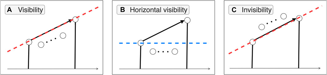
FIGURE 1. Graphical distinction among subclasses of family of visibility algorithms. (A) The visibility criterion (Eq. 2.1) requires all nodes between the from node and the to node to stand below the dashed red line. (B) The horizontal visibility criterion (Eq. 2.2) requires all the between nodes to be below the dashed blue line. (C) The invisibility criterion (Eq. 2.9) requires all the between nodes to be on or above the dashed red line.
The horizontal visibility graph (HVG)
Note that horizontal visibility criterion is a sufficient condition for the visibility criterion, i.e.,
Notations
After a time series is mapped into a directed network (
An important remark here is that an ingoing edge is counted as an outgoing edge if viewed from the reversed time horizon; thus, ingoing and outgoing degree sequences are interchangeable under the time-reversal transformation:
The identity of Eq. 2.3, which is common among the family of visibility graph algorithms, is crucially important when later we define the measurement of the time (ir)reversibility.
Next, let us define the ingoing and outgoing degree distributions of
As a result, the property of Eq. 2.3 can be formulated in terms of the degree distributions:
Quantifying the Time (Ir)reversibility
As stated at the beginning of this paper, the time reversibility of a time series stands for the invariance of properties under the time-reversal transformation. Hence, to quantify the time irreversibility, we need to compare the property of the original series with its time-reversed counterpart. With the language of VG or HVG, one may compare ingoing (outgoing) degree distribution of the original time series
A time series of length
For time series of a finite size, we can assess the degree of time (ir)reversibility, namely, how much time-(ir)reversible the series is, by the quantitative measurement of the distance between
KLD is defined as a semi-distance that vanishes if and only if the two probability distributions are identical and has a positive value otherwise. KLD is not only convenient to quantify the distance between probabilities but also significant in statistical mechanics, in such a way that it can be used to estimate the average entropy production of the associated system [7]. Here, the measured value is the KLD between probability distributions associated with observables (e.g., time series, network) obtained from a certain process and its time reversal.
One additional technical remark is that Eq. 2.7 may diverge when one or more degree
Such that
Since degree distributions derived from an actual time series would fluctuate with its size, in practice, we will measure the speed of decay of the measure (
Refinement of the Method
Intuitions
As our refinement of the VG algorithm is based on the hypothesis made in Introduction that the topology of trajectories stores all the information of time series, what we need to do is to capture the topological properties of time series and to effectively quantify the time (ir)reversibility.
First, let us describe the proposed procedure to capture the topological properties of a time series:
1. Set a moving time window and divide the whole series into a sequence of overlapping trajectories with the fixed length of the time window.
2. Identify the geometric properties of each trajectory of the time series in the moving windows.
3. Aggregate the geometric properties of each piece to evaluate the geometric property of the whole series.
The primary issue regards what characteristics we need to tell apart. Here, we discriminate trajectories based on direction (rise or fall) as well as the shape (convex, concave, or otherwise). Note that the shape of a trajectory’s geometry is difficult to define merely via statistical approaches because realized trajectories are the convolution of different temporal modes [31]. Hence, we keep employing the family of visibility algorithms; in the meantime, we also try to give a remedy to deficiencies of the VG-based or HVG-based method. Specifically, besides the visibility criterion, we also employ the invisibility criterion to construct the network from a time series, because both criteria can reflect the convexity and concavity of functions in a straightforward manner. Note that the visibility of two distant data points directly relates to the convexity of a trajectory, and the invisibility relates to the concavity.
The invisibility criterion here refers to the algorithm introduced by Yan et al., named as the “absolute invisibility algorithm” [27], which is just the opposite of the visibility criterion (Eq. 2.1).
A pair of nodes,
where, again,
Visibility Graph With Colored Edges
We construct a new kind of visibility graph, “the degree-vector-based visibility graph” (DV-VG hereafter), from a time series
1. The neighborhood condition [27]
where
2. The direction and shape condition
• Rise and Visible (RV) (for
where
• Rise and Invisible (RIV) (for
• Fall and Visible (FV) (for
• Fall and Invisible (FIV) (for
To summarize, the neighborhood condition, Eq. 2.10, should be satisfied for all types of edges, while one of the four conditions for direction and shape (i.e., Eqs 2.11.14.–.Eqs 2.2.14) needs to be satisfied depending on the color of edges. See Figure 2 for a graphical illustration of the distinction among the criteria for different
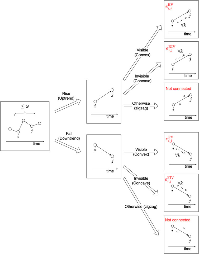
FIGURE 2. Graphical illustration of the edge criteria to construct the degree-vector-based visibility graph (DV-VG). Any pair of nodes,
Owing to the neighborhood condition, a node in DV-VG can at most have
The Degree Vector
Let us prepare some notations for the description of properties of DV-VG.
First, let
Similarly, we can define
To define time reversibility with the use of ingoing and outgoing degree vectors of the DV-VG representations, we need to hold the symmetry between the ingoing and the outgoing degree vector under the time-reversal transformation, namely,
Among the three conditions for the construction of DV-VG described in Visibility Graph With Colored Edges, the neighborhood criterion and the shape (visibility/invisibility) criteria are not altered through the time-reversal transformation. In contrast, as shown in Figure 3, the upward trend along with the original time direction would become a downward trend when viewed from the opposite time horizon. In other words, the direction criterion for of DV-VG is reversed under the time-reversal transformation. Thus, to keep the time-reversal property (Eq. 2.16), components of the outgoing degree vector need to be permuted as:
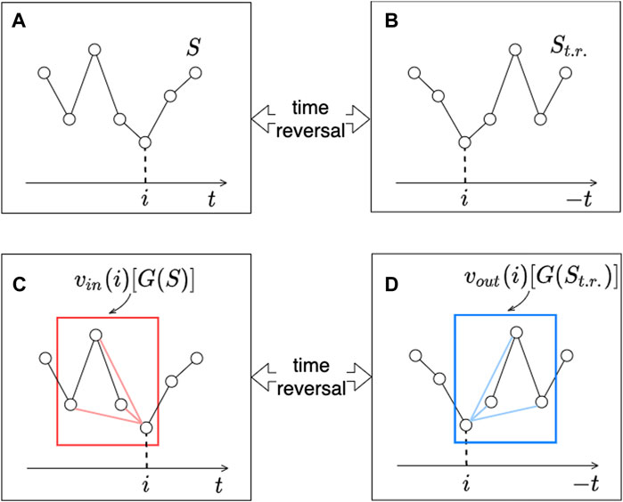
FIGURE 3. Graphical confirmation of the definition of
The difference in the order of four elements composing
Interpretations of the Degree Vector
The ingoing degree vector at time
As a concrete example, Figure 4 shows the relationship between the ingoing degree vectors and the corresponding geometric patterns in the case of
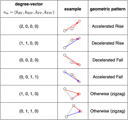
FIGURE 4. The relationship between ingoing degree vectors, examples of corresponding realizations of trajectories, and the corresponding geometric patterns (in the case with
Quantifying the Time (ir)reversibility
As we have converted the time series into a sequence of degree vectors that correspond to specific geometric patterns for each piece of the local trajectories of index motion, let us define the distributions of ingoing or outgoing degree vectors for DV-VG constructed from
Note that the property indicated in Eq. 2.16 shall be inherited to the degree vector distributions. Hence, DG-VG, by definition [i.e., regardless of the existence of the time (ir)reversibility], holds the following equality properties:
Based on this symmetry between ingoing and outgoing degree distributions under time-reversal transformation, we generalize a new working definition of time reversibility:
A time series
For the time series with a finite size, however, we can assess how much the time series is time-(ir)reversible through quantifying the distance between distribution
On the specific meaning of KLD, see Quantifying the Time-(Ir)reversibility. As is the case with previous methods, since degree vector distributions derived from an actual time series fluctuate with its size, we measure the speed of decay of the measure
Discussions on DV-VG
The proposed working definition of time reversibility with the use of DV-VG is essentially a topological description such that it quantifies the similarity between the original and reversed time series in terms of the occurrence distributions of short-length geometric patterns. The topological time reversibility does not necessarily require the identical joint distribution for
The distinctive aspects of DV-VG compared to the original visibility graph (VG) method lie in twofold:locality and detailedness.
As the first characteristic, DV-VG uses local rather than global information. In contrast, the VG mapping from a time series to network is done by using the whole series [25]. We propose this division of the whole series into a sequence of the local subseries based on the fact that the aggregation of local trajectories should certainly include the information of the whole series. This locality, as we will show in Section 3.1.3, enables us to preclude the effect of non-ergodicity when analyzing multiplicative random walks. Additionally, the idea of focusing on local information when coarse graining the series provides us some conveniences. First, it requires a much lower computational cost. The computational cost for the construction of VG with a naïve algorithm increases as
The second characteristic of DV-VG is that it contains more detailed information about the topological properties of trajectories. When mapping a data point
Validation of DV-VG
In this section, we first validate DV-VG via the measurement of time irreversibility for time series generated by numerical simulations. Furthermore, we shall employ DV-VG to investigate the properties of real-world financial time series.
As is explained in Discussions on DV-VG, the distinctive features of DV-VG refer to both locality and detailedness of the mapping procedure. The effectiveness of DV-VG needs to be demonstrated through comparisons of different methods. To ensure the fairness of such comparisons, besides VG, we further employed a modified VG equipped with the locality of DV-VG. In particular, a localized VG;
In the following section, we shall apply three methods, i.e., VG, LVG, and DV-VG, to measure time irreversibility of a set of synthetic time series. Note that we set
1. White Noise:
2. Chaotic logistic map:
3. Unbiased additive random walk:
4. Additive random walk with positive drift:
5. Additive random walk with memory effect (non-Markovian random walk):
6. Unbiased multiplicative random walk:
7. Multiplicative random walk with negative drift:
8. GARCH (1, 1) process:
Stationary Processes
We first consider two canonical stationary processes: White noise and Chaotic logistic map. Figure 5 shows the time irreversibility of (A) White noise and (B) Chaotic logistic map as a function of the time series length
(A) White noise
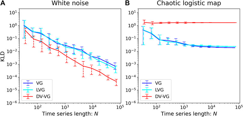
FIGURE 5. Log–log plot of the time irreversibility, KLD, of (A) white noise and (B) chaotic logistic map as a function of the time series length
In all the three results, the measured KLD decays asymptotically as
(B) Chaotic logistic map
Via all the three measurement methods, the convergence of KLD to a finite and positive value is shown as the size of the time series increases, thus the process is categorized as time-irreversible. Note that measurement by DV-VG is insensitive to the size of time series.
To summarize, our results are in good agreement with previous theory, in which the white noise is, by definition, time-reversible, and the chaotic map is, also by definition as a dissipative chaotic process, time-irreversible.
Additive Random Walks
Figure 6 shows the time irreversibility of (A) Unbiased Additive Random Walks (ARW), (B) ARW with positive drift, and (C) Unbiased ARW with memory effects as a function of the time series length. Comments are provided as follows.
(A) Unbiased ARW
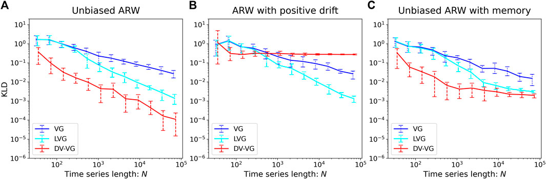
FIGURE 6. Log–log plot of the time irreversibility, KLD, of (A) unbiased, (B) positively biased, and (C) non-Markovian additive random walk as a function of the time series length
In all the three cases, KLD vanishes asymptotically as
(B) ARW with positive drift
For VG and LVG, the measured KLD vanishes asymptotically, implying that the process is time-reversible. This erroneous result owes to the visibility criterion (not the trend condition) being invariant under the addition of linear trends [7]. In contrast, the measured KLD via DV-VG converges to a finite value manifesting that the trending motion of the time series brings about the time irreversibility. The reason for DV-VG to distinguish a trend is clear: the differentiation of rising (uptrend) and falling (downtrend) trajectories have been taken into account when constructing the degree vectors.
(C) Unbiased ARW with memory effect
Similar to case (B), the measurement via VG or LVG breeds a decreasing KLD as the series size gets larger, while the measurement via DV-VG results in the KLD converging to a finite positive value. By differentiating geometric patterns more precisely, our new method alone can successfully distinguish the existence of memory effects on additive random walk as a source of the time irreversibility.
Multiplicative Random Walks
Figure 7 shows the time irreversibility of (A) Unbiased Multiplicative Random Walks (MRW), (B) MRW with negative drift, and (C) GARCH (Generalized auto-regressive conditional heteroscedasticity), i.e., unbiased MRW with volatility clustering, as a function of the time series length.
(A) Unbiased MRW
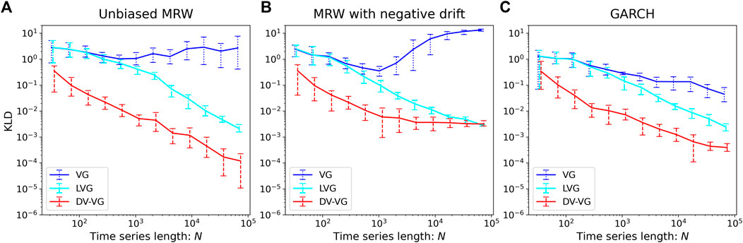
FIGURE 7. Log–log plot of the time irreversibility, KLD, of (A) unbiased, (B) negatively biased multiplicative random walk, and (C) GARCH as a function of the time series length
In the case of the VG, the measured KLD does not vanish along with the increase of series length, indicating the time-irreversible nature. In contrast, in the cases of the LVG and DV-VG, as KLD vanishes asymptotically, the process is judged as time-reversible. Here, the result differs depending on the measurement methods employed. The multiplicative random walk is known to have a non-ergodic nature and contains extremely rare but extremely different events. In the case of the original VG, a node will be connected to all the visible nodes no matter how far away they are. As the non-ergodicity of MRW is inherited, the degree distribution will be dominated by extreme events. In other words, the degree distribution has a fat tail resulting from the large fluctuation over realizations [7]. If we add the neighborhood condition, thus cut off the impact of extreme events, the non-ergodicity of MRW itself shall not be inherited to the degree distribution or degree vector distribution of its graph representations. As a result, the time irreversibility measure vanishes with
(B) MRW with negative drift
The KLD value computed via the VG does not vanish with the series length as is the case in the unbiased MRW. In contrast, the KLD value computed via LVG vanishes asymptotically as about
(C) GARCH
The GARCH model is a typical extension of the MRW that can model the tendency of large changes to cluster in log-returns of index [16], which is typically called volatility clustering and is known as one of the stylized facts of financial time series. Since the process contains additional directional information, GARCH should be more time-irreversible than the unbiased MRW. First, in the case of VG, the measured KLD does not decrease and rather starts fluctuating strongly as the series’ length gets longer. Although it seems that VG is capable of capturing the time irreversibility of the GARCH model, it is not clear whether the measure captures the time-irreversible nature, which is rooted in the volatility clustering since VG has produced an erroneous non-vanishing KLD in the unbiased MRW. Second, in the case of LVG, the KLD vanishes asymptotically, suggesting that the method fails to detect GARCH’s time irreversibility. Finally, the KLD obtained through DV-VG does not vanish and converges to a finite value with a large
Discussion
As shown in the previous subsections, we have tested the capability of different methods for the measurement of time reversibility for a set of synthetic time series that are generated from eight canonical processes. Among these test cases, the newly proposed DV-VG method can yield a renormalized time irreversibility measure, which vanishes asymptotically if the process is unbiased (in the logarithmic space for the multiplicative random walks) or converges to a finitely positive value if the process contains linear trend, memory effect, or volatility clustering. Note that the previous method (i.e., VG) fails in detecting non-Markovianity within the class of additive random walk. Again, the reason why DV-VG is superior to its original version is that one can examine in detail whether certain geometric patterns occur more/less frequently in the forward series;
Demonstrations of Real Stock Indices
In this section, we further demonstrate the capability of DV-VG by exploratorily analyzing the time (ir)reversibility of financial time series generated from real markets. Specifically, we have investigated time (ir)reversibility of stock indices of six representative financial markets:
1. Japanese Nikkei 225 (N225)
2. Indian Bombay Stock Exchange Sensitive Index (SENSEX)
3. Hong Kong Hang Seng Index (HSI)
4. French CAC 40 (CAC 40)
5. Dow Jones Industrial Average (DJI)
6. German DAX (DAX)
We use the daily closing price during the period from June 28, 1999 to June 28, 2019, which yields around
One important note here is that raw values [i.e.,
The precise methodology (for the analysis of each index price) is described as follows.
1) We construct a working time window of
2) For each of these sub-series, we construct the associated DV-VG and compute the KLD via its degree vector distributions.
3) We also calibrate7 the parameter of GARCH (1, 1) by fitting the model to the log-return (i.e.,
4) Using calibrated parameters and GARCH (1, 1) model, we regenerate a sample price time series with the length
5) We compute the mean level time irreversibility of the associated GARCH (1, 1) process via a Monte Carlo simulation, by repeating 4) 50 times and calculating the mean and the standard deviation of the aggregated results.
6) Finally, we compare the level of time irreversibility obtained from the real data with the associated GARCH (1, 1) model.
Figure 8 shows the degree-vector-based time irreversibility plotted as a function of date. Each data point of thick red lines denotes the time irreversibility of last
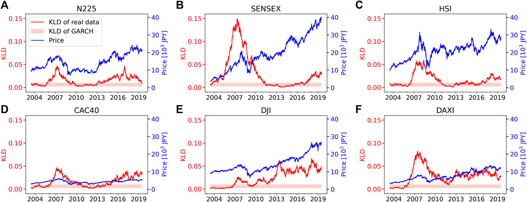
FIGURE 8. The index motion and the measured time irreversibility via DV-VG, as a function of date. The blue line denotes price of the index. The red solid line denotes KLD associated with the real data. The pink shaded area denotes KLD from the GARCH (1, 1) model (mean
Overall, three observations should be noted: 1) all the index series can be judged as time-irreversible as a whole, but 2) the degree of the time irreversibility varies across indices and 3) the degree of time irreversibility also varies over time, which are in good accordance with the previous research [21]. Besides these observations, there are several findings from our results. First, the KLD values from any indices are significantly larger than those constructed from the unbiased multiplicative random walk (with the same length:
Conclusion
Let us remind readers that the main objective of our study is to answer the following two questions:
Research Question 1.
How can we capture the topological properties of time series?
Research Question 2.
How can we quantitatively measure the time irreversibility from the topological perspective?
As for the answer to the first question, the newly defined “degree vector” has enabled us to characterize the topological property of each piece of the local (short) trajectories. The degree vector can be determined with three different geometrical criteria, namely, 1) the neighborhood condition, 2) the trend condition, and 3) the shape condition. With respect to the shape condition, we utilized visibility and invisibility algorithms for the classification of different kinds of edges. In summary, our answer to the RQ1 is that the proposed degree vector at
Regarding the second question, a new measurement method for the time irreversibility of time series is proposed based on the degree vector representation, i.e., DV-VG. To validate the new measurement method, the results of the measurement of the numerical simulation of eight classes of synthetic time series are compared with those of the other measurement methods, that is, VG and LVG. By using DV-VG, we successfully detect the time-irreversible nature rooted in 1) linear trends and 2) memory effects (i.e., non-Markov property), which are not detectable via the other two methods. Hence, although we are not yet able to provide exact mathematical proofs, we may answer RQ2 as “yes” with the current numerical evidence. Furthermore, we have applied DV-VG to time series generated from the GARCH model, which is a basic extension of the unbiased multiplicative random walk to model financial time series. The degree-vector-based time irreversibility does not vanish and converges to a finite value with large enough
As a preliminary study, we further applied DV-VG to six stock index time series from canonical real markets and compared the results with the calibrated GARCH (1, 1) model in terms of the time irreversibility. Interestingly, we found that the GARCH (1,1) model can reproduce the time irreversibility only during certain periods; the degree of time irreversibility of the real stock indices measured by DV-VG is much higher out of these periods. This result suggests that though the GARCH model has become a mature model of real-world stock indices in general, it still lacks the capability in capturing the time irreversibility of financial time series.
As the final remark, we propose three possible applications of our method (i.e., the degree vector) for the future investigation. First, we can search specific geometric patterns from time series by employing the degree vector. For example, if the accelerated rise in a time series is of interest, one can search the degree vectors with large
Data Availability Statement
The datasets presented in this study can be found in an online repository (https://github.com/ryutau/refined-time-irreversibility).
Author Contributions
RM, RL, and YC contributed to the conception of the study; RM performed the data analyses and wrote the article; RL and CY helped perform the analyses with constructive discussions.
Conflict of Interest
The authors declare that the research was conducted in the absence of any commercial or financial relationships that could be construed as a potential conflict of interest.
Publisher’s Note
All claims expressed in this article are solely those of the authors and do not necessarily represent those of their affiliated organizations, or those of the publisher, the editors and the reviewers. Any product that may be evaluated in this article, or claim that may be made by its manufacturer, is not guaranteed or endorsed by the publisher.
Supplementary Material
The Supplementary Material for this article can be found online at: https://www.frontiersin.org/articles/10.3389/fphy.2021.777958/full#supplementary-material
Footnotes
1More precisely, for time series obtained from stochastic processes (e.g., random walk) to be predictable, at least it must be somewhat time irreversible. In the case of the deterministic process, on the other hand, the concept of predictability is not applicable, and the time irreversibility implies the existence of an exact seasonal cycle in the process
2Although the original version of the (horizontal) visibility graph was first introduced as an undirected graph, later it is extended to a directed graph [25], in which the direction of nodes is defined according to the direction of time. In the context of the time irreversibility, we always refer to the directed version of (horizontal) visibility graphs
3In the following section, we use the notation
4We chose comparatively large
5We checked the results with
6Here, we set
7“Arch” package [34] (https://arch.readthedocs.io/en/latest/) in python is employed to estimate the three parameters of GARCH (1, 1).
References
1. Lawrance AJ. Directionality and Reversibility in Time Series. Int Stat Rev/Revue Internationale de Statistique (1991) 59:67. doi:10.2307/1403575
2. Zumbach G. Time Reversal Invariance in Finance. Quantitative Finance (2009) 9:505–15. doi:10.1080/14697680802616712
3. Lamb JSW, Roberts JAG. Time-reversal Symmetry in Dynamical Systems: A Survey. Physica D: Nonlinear Phenomena (1998) 112:1–39. doi:10.1016/S0167-2789(97)00199-1
4. Andrieux D, Gaspard P, Ciliberto S, Garnier N, Joubaud S, Petrosyan A. Entropy Production and Time Asymmetry in Nonequilibrium Fluctuations. Phys Rev Lett (2007) 98:98–101. doi:10.1103/PhysRevLett.98.150601
5. Prigogine I, Antoniou I. Laws of Nature and Time Symmetry Breaking. Ann NY Acad Sci (1999) 879:8–28. doi:10.1111/j.1749-6632.1999.tb10402.x
6. Puglisi A, Villamaina D. Irreversible Effects of Memory. Europhys Lett (2009) 88:30004. doi:10.1209/0295-5075/88/30004
7. Lacasa L, Flanagan R. Time Reversibility from Visibility Graphs of Nonstationary Processes. Phys Rev E (2015) 92:022817. doi:10.1103/PhysRevE.92.022817
8. Costa M, Goldberger AL, Peng C-K. Broken Asymmetry of the Human Heartbeat: Loss of Time Irreversibility in Aging and Disease. Phys Rev Lett (2005) 95:2–5. doi:10.1103/PhysRevLett.95.198102
9. Kaldor N. Capital Accumulation and Economic Growth. In: DC Hague, editor. The Theory of Capital: Proceedings of a Conference Held by the International Economic Association. London: Palgrave Macmillan UK (1961). p. 177–222. doi:10.1007/978-1-349-08452-4_10
10. Cont R. Empirical Properties of Asset Returns: Stylized Facts and Statistical Issues. Quantitative Finance (2001) 1:223–36. doi:10.1080/713665670
11. Chakraborti A, Toke IM, Patriarca M, Abergel F. Econophysics Review: I. Empirical Facts. Quantitative Finance (2011) 11:991–1012. doi:10.1080/14697688.2010.539248
12. Rachev ST, Menn C, Fabozzi FJ. Fat-tailed and Skewed Asset Return Distributions: Implications for Risk Management, Portfolio Selection, and Option Pricing. New Jersey, US: John Wiley & Sons (2005).
13. Verhoeven P, McAleer M. Fat Tails and Asymmetry in Financial Volatility Models. Mathematics Comput Simulation (2004) 64:351–61. doi:10.1016/S0378-4754(03)00101-0
14. Mandelbrot B. The Variation of Certain Speculative Prices. J Bus (1963) 36:394. doi:10.1086/294632
15. Romero DM, Meeder B, Kleinberg J “Differences in the Mechanics of Information Diffusion across Topics: Idioms, Political Hashtags, and Complex Contagion on Twitter.” in WWW 2011 Proc 20th Int Conf World Wide Web, 2011 March 28-April 1; Hyderabad India (2011). 695–704. doi:10.1145/1963405.1963503
16. Cont R. Volatility Clustering in Financial Markets: Empirical Facts and Agent-Based Models. Long Mem Econ (2007) 289–309. doi:10.1007/978-3-540-34625-8_10
17. Lux T, Marchesi M. Volatility Clustering in Financial Markets: a Microsimulation of Interacting Agents. Int J Theor Appl Finan (2000) 03:675–702. doi:10.1142/s0219024900000826
18. Niu H, Wang J. Volatility Clustering and Long Memory of Financial Time Series and Financial price Model. Digital Signal Process. (2013) 23:489–98. doi:10.1016/j.dsp.2012.11.004
19. Andersen TG, Bollerslev T. Intraday Periodicity and Volatility Persistence in Financial Markets. J Empirical Finance (1997) 4:115–58. doi:10.1016/S0927-5398(97)00004-2
20. Eom C, Oh G, Jung W-S. Relationship between Efficiency and Predictability in Stock price Change. Physica A: Stat Mech its Appl (2008) 387:5511–7. doi:10.1016/j.physa.2008.05.059
21. Flanagan R, Lacasa L. Irreversibility of Financial Time Series: A Graph-Theoretical Approach. Phys Lett A (2016) 380:1689–97. doi:10.1016/j.physleta.2016.03.011
22. Zanin M, Rodríguez-González A, Menasalvas Ruiz E, Papo D. Assessing Time Series Reversibility through Permutation Patterns. Entropy (Basel) (2018) 20:1–15. doi:10.3390/e20090665
23. Lacasa L, Luque B, Ballesteros F, Luque J, Nuño JC. From Time Series to Complex Networks: The Visibility Graph. Pnas (2008) 105:4972–5. doi:10.1073/pnas.0709247105
24. Luque B, Lacasa L, Ballesteros F, Luque J. Horizontal Visibility Graphs: Exact Results for Random Time Series. Phys Rev E (2009) 80:1–11. doi:10.1103/PhysRevE.80.046103
25. Lacasa L, Nuñez A, Roldán É, Parrondo JMR, Luque B. Time Series Irreversibility: A Visibility Graph Approach. Eur Phys J B (2012) 85:217. doi:10.1140/epjb/e2012-20809-8
26. Hu J, Xia C, Li H, Zhu P, Xiong W. Properties and Structural Analyses of USA's Regional Electricity Market: A Visibility Graph Network Approach. Appl Maths Comput (2020) 385:125434. doi:10.1016/j.amc.2020.125434
27. Yan W, Van Tuyll Van Serooskerken E. Forecasting Financial Extremes: A Network Degree Measure of Super-exponential Growth. PLoS One (2015) 10:e0128908–15. doi:10.1371/journal.pone.0128908
28. Xiong H, Shang P, Hou F, Ma Y. Visibility Graph Analysis of Temporal Irreversibility in Sleep Electroencephalograms. Nonlinear Dyn (2019) 96:1–11. doi:10.1007/s11071-019-04768-2
29. Zanin M, Güntekin B, Aktürk T, Hanoğlu L, Papo D. Time Irreversibility of Resting-State Activity in the Healthy Brain and Pathology. Front Physiol (2020) 10:1619. doi:10.3389/fphys.2019.01619
30. González-Espinoza A, Martínez-Mekler G, Lacasa L. Arrow of Time across Five Centuries of Classical Music. Phys Rev Res (2020) 2:033166. doi:10.1103/PhysRevResearch.2.033166
31. Liu R, Chen Y. Analysis of Stock Price Motion Asymmetry via Visibility-Graph Algorithm. Front Phys (2020) 8:1–13. doi:10.3389/fphy.2020.539521
32. Lan X, Mo H, Chen S, Liu Q, Deng Y. Fast Transformation from Time Series to Visibility Graphs. Chaos (2015) 25:083105. doi:10.1063/1.4927835
33. Okimoto T. [Econometric Time Series Analysis of Economic and Financial Data] Keizai Fainance Deta No Keiryo Jikeiretsu Bunseki. Tokyo: Asakura Publishing (2010). (in Japanese).
Keywords: time series analysis, time-reversibility, visibility graph, time series motifs, time series similarity
Citation: Mori R, Liu R and Chen Y (2021) Measuring the Topological Time Irreversibility of Time Series With the Degree-Vector-Based Visibility Graph Method. Front. Phys. 9:777958. doi: 10.3389/fphy.2021.777958
Received: 16 September 2021; Accepted: 14 October 2021;
Published: 12 November 2021.
Edited by:
Haroldo V. Ribeiro, State University of Maringá, BrazilReviewed by:
Max Jauregui, Universidade Estadual de Maringá, BrazilChengyi Xia, Tianjin University of Technology, China
Copyright © 2021 Mori, Liu and Chen. This is an open-access article distributed under the terms of the Creative Commons Attribution License (CC BY). The use, distribution or reproduction in other forums is permitted, provided the original author(s) and the copyright owner(s) are credited and that the original publication in this journal is cited, in accordance with accepted academic practice. No use, distribution or reproduction is permitted which does not comply with these terms.
*Correspondence: Ryutaro Mori, cnl1dGF1Lm1vcmlAZ21haWwuY29t; Yu Chen, Y2hlbkBlZHUuay51LXRva3lvLmFjLmpw