A New Modified Analytical Approach for the Solution of Time-Fractional Convection–Diffusion Equations With Variable Coefficients

In this article, a new modification of the Adomian decomposition method is performed for the solution fractional order convection–diffusion equation with variable coefficient and initial–boundary conditions. The solutions of the suggested problems are calculated for both fractional and integer orders of the problems. The series of solutions of the problems with variable coefficients have been provided for the first time. To verify and illustrate our new technique, four numerical examples are presented and solved by using the proposed technique. The derived results are plotted, and the dynamics are shown for both fractional and integer orders of the problems. An excellent variation among the solutions at various fractional orders is observed. It is analyzed that the new technique based on the Adomian decomposition method is accurate and effective. The present method fits both the initial and boundary conditions with double approximations simultaneously, which increases the accuracy of the present method. For the first time, the present technique is used for the solutions of the problems with variable coefficients along with initial and boundary conditions. It is therefore suggested to apply the present procedure for the solutions of other problems with variable order and coefficients along with initial and boundary conditions.

1 Introduction

Fractional Calculus (FC) is the branch of mathematics that focuses on the study of fractional-order operators and their applications in mathematical theory, which is the expansion of the basic classical concept in calculus and has attracted the attention of many researchers in the last few decades. FC has useful applications in numerous fields of physical and numerical sciences, such as relaxation processes, diffusion, visco-elasticity, hydrology, biomedical engineering, electro-chemistry, relaxation vibration, finance, probability, seismology, and so on [1–5]. Other FC applications include earthquake’s oscillations modeling [6], statistical and mechanic continuum [7], control theory [8], engineering and physics [9, 10], entropy [11], image processing [10], field theories, optimal control, classical and quantum mechanics [12, 13], chaos theory [14], fractional diabetes model [15], and human diseases [16]. The main contribution to the development of (FC) includes Podlubny et al. [17]; Miller and Ross [18]; Oldham and Spanier [19]; and Kilbas and Trujillo [20].

A well-known fact about fractional-order partial differential equations (FPDESs) is that they are involved in many natural and physical phenomena. Many researchers have attracted towards them due to the wonderful applications in various fields especially anomalous diffusion, dielectric polarization, relaxation vibration, scattering, system identification, fluid flow, mathematical physics [21], psychology, and acoustics [22].

Over the last 10 years, attempts were made to find robust analytical and numerical techniques to solve (FPDES). Some of them are the homotopy analysis method [23], the wavelet operational method [24, 25], the Legendre-based method [26], the fractional recti sub-equation method [27], the generalized fractional Taylor series method [28], the Laplace Adomian decomposition method [29], the fractional wavelet method [30], the Adomian decomposition method [31], the discrete Adomian decomposition method [32], the Mohand decomposition method [33], the Wlash function method [34], the Chebyshev spectral approximation [35], the wavelet optimization method [36], the solitary ansatz method [37], the multiple exp-function method [38], the Hirotas direct method [39], the Laplace transform decomposition method [40], the natural transform decomposition method [41], and so on. The time-fractional convection–diffusion equations (CDESs) have been conventional used in the mathematical models of computations and simulations, such as the transport of energy and mass, oil reservoir simulations, flow of heat, particles, dispersion of chemicals in reactors, and global weather prediction [42, 43]. Time-fractional CDEs are operated in the abnormal diffusion processes related to time.

Several research work have been done on the Adomian decomposition method (ADM), such as Wazwaz A.M. [44] used it to solve linear and non-linear operators, initial-value problems solved by Abdelrazec and Pelinovsky [45] and Ray and Bera [46] applied it to the differential equations. Hashim [47] applied it to the boundary-value problems, fractional differential equations solved by Hu and Luo [45], Duan J.S. applied to the boundary-value problems [48], Song and Wang [49] solved fractional differential equations, initial value problems solved by Wu [50] and Almazmumy et al. [51]. Patel et al. applied the ADM sumudu transform method in [52, 53] and the fractional reduced differential transform method in [54, 55]. For the convergence of ADM, see [56, 57]. Fatoorehchi et al. solved explicit Frost–Kalkwarf type equations by ADM [58]. The one thing about all the above appreciable work is that ADM is used either with initial or only boundary conditions. Furthermore, a new modification is generated in ADM by Ali in [31, 59] for initial–boundary problems. He used the same new technique in [60] with the variation iteration method, and the results are good. We extend his work by applying it to fractional order problems. This procedure gives accuracy because we construct a new initial approximate for each iteration. Abdelrazec et al. have provided a comprehensive study on the convergence of ADM for initial value problems in [61]. Similarly, Aminataei et al. have done the stability of ADM with other methods in [62].

In the present work, time-fractional CDEs with variable coefficients are considered as follows:

$\frac{{\partial }^{\gamma }u\left(\zeta ,t\right)}{\partial t^{\gamma }}+c\left(\zeta \right)\frac{\partial u\left(\zeta ,t\right)}{\partial \zeta }+d\left(\zeta \right)\frac{{\partial }^{2}u\left(\zeta ,t\right)}{\partial {\zeta }^2}=\kappa \left(\zeta \right),0<\zeta <1,0<t\le 1,$

with the initial conditions

$u\left(\zeta ,0\right)=f\left(\zeta \right),0<\zeta <1,$

and the boundary conditions

$u\left(0,t\right)=g_0\left(t\right),u\left(1,t\right)=g_1\left(t\right)0<t\le 1,$

where c(ζ), d(ζ) ≠ 0 are continuous functions and 0 < γ < 1. The fractional derivative is in the Caputo sense.

Many techniques have been used to obtain the solutions of time-fractional CDEs such as the Gegenbauer spectral method [63], the Sinc–Legendre collocation method [64], the Bernstein polynomials method [65], the flatlet oblique multi wavelets [66], and the improved differential transform method [67]. Marjan et al. applied the radial basis interpolation method to compute the solution of this equation with constant coefficients [68]. Luo et al. computed the equation by the quadratic spline collocation method with constant coefficient and without convection [69]. In [70], Pirkhedri and Javadi computed the equations with variable coefficient by the collocation approach.

In this article, we have investigated the analytical solutions of various time-fractional CDEs by using a new technique of the Adomian decomposition method (ADM). In the year 1980, Adomian had developed an effective technique, called ADM to solve differential equations involved in physical phenomena [71]. Later on, some short coming related to ADM, the researchers have modified ADM and construct some effective tools for the solutions of various fractional partial differential equations and their systems. Generally, many techniques are not efficient for the solutions of fractional initial and boundary conditions together. However, in this work, the solutions of initial and boundary value problems related to time-fractional CDEs are obtained by using a new technique of ADM. The obtained solutions are represented through graphs and tables. The 2D and 3D graphs have confirmed a closed contact between the exact and new version of ADM results. The fractional-order solutions represent the valuable dynamics of the suggested problems. The solution convergence of the fractional solutions towards integer-order solutions confirmed the validity of the suggested method. The present method is simple and required fewer calculations and therefore can be extended for the solutions of other higher non-linear fractional PDEs and their systems.

2 Preliminaries

In this section, a few definitions related to our work are taken into consideration.

2.1 Definition

The expression for the Caputo derivative of fractional order γ is as follows:

$\left(D^{\gamma }h\right)\left(\zeta \right)=\frac{{\partial }^{\gamma }h\left(\zeta \right)}{\partial t^{\gamma }}=\left\{\begin{array}{c}{I}^{p-\gamma }\left[\frac{{\partial }^{\gamma }h\left(\zeta \right)}{\partial t^{\gamma }}\right],p-1<\gamma \le p,\hfill \\ \frac{{\partial }^{\gamma }h\left(\zeta \right)}{\partial t^{\gamma }},\hfill \end{array}\right.$

where $p\in \mathbb{N}$, ζ > 0, $g\in {\mathbb{C}}_t$, and t ≥ 1.

2.2 Definition

The Reimann–Liouville integral operator having order γ is given by [72]

$\left(I_{\zeta }^{\gamma }h\right)\left(\zeta \right)=\left\{\begin{array}{cc}\frac{1}{\mathrm{\Gamma }\left(\gamma \right)}{\int }_0^{\zeta }{\left(\zeta -\nu \right)}^{\gamma -1}d\nu ,\hfill & \gamma >0,\hfill \\ h\left(\zeta \right),\hfill & \gamma =0,\hfill \end{array}\right.$

where Γ denotes the gamma function and can be written as

$\mathrm{\Gamma }\left(\omega \right)={\int }_0^{\infty }{e}^{-\zeta }{\zeta }^{\omega -1}d\zeta ,\omega \in \mathbb{C}.$

2.3 Lemma

For p − 1 < γ ≤ p with $p\in \mathbb{N}$ and $h\in {\mathbb{C}}_t$ with t ≥ −1, then [73].

$\left\{\begin{array}{c}{I}^{\gamma }{I}^b=I^{\gamma +b}h\left(\zeta \right),b,\gamma \ge 0,\hfill \\ I^{\gamma }{\zeta }^{\lambda }=\frac{\mathrm{\Gamma }\left(\lambda +1\right)}{\mathrm{\Gamma }\left(\gamma +\lambda +1\right)}{\zeta }^{\gamma +\lambda },\gamma >0,\lambda >-1,\hfill \\ I^{\gamma }{D}^{\gamma }h\left(\zeta \right)=h\left(\zeta \right)-\sum _{k=0}^{p-1}{h}^k\left(0^{+}\right)\frac{{\zeta }^k}{k!},\hfill \end{array}\right.$

where ζ > 0 and p − 1 < γ ≤ p.

2.4 Definition

The Mittag-Leffler function E_γ(ρ) for γ > 0 is [74]

$E_{\gamma }\left(\rho \right)=\sum _{n=0}^{\infty }\left(\frac{{\rho }^n}{n\gamma +1}\right),\gamma >0,\rho \in \mathbb{C}.$

3 Adomian Decomposition Method

This method was discovered by Adomian for the solution of linear and nonlinear differential and integro-differential equations. To understand about the method, consider the following equation [31]:

$F\left(u\left(\zeta \right)\right)=g\left(\zeta \right),(1)$

where g is the known function and F (u(x)) is the differential operator, which can be decomposed as follows:

$F\left(u\left(\zeta \right)\right)=Lu+Ru+Nu,$

where L is the invertible operator of highest order derivative, R represents the linear operator, and N is the non-linear term. Then, Eq. (1) has the following representation:

$Lu+Ru+Nu=g.(2)$

Apply the inverse operator L⁻¹ on both sides of Eq. (2),

$u=\phi +L^{-1}\left(g\right)-L^{-1}\left(Ru\right)-L^{-1}\left(Nu\right),$

where φ is the constant of integration and Lφ = 0.The ADM solution is represented as an infinite series,

$u=\sum _{n=0}^{\infty }{u}_n.$

The non-linear term Nu is denoted by A_n and is defined as follows:

$Nu=\sum _{n=0}^{\infty }{A}_n.$

With the help of the following formula, we can calculate A_n as

$A_n=\frac{1}{n!}\frac{d^n}{d{\psi }^n}N\left(\sum _{k=0}^{\infty }\left({\psi }^k{u}_k\right)\right),n=\mathrm{0,1},\dots .$

The other method to calculate Adomian polynomials can be seen in [75]. The series has the following relation to represent the solution of Eq. (1):

$\left\{\begin{array}{cc}\hfill & u_0=\phi +L^{-1}\left(g\right),n=0,\hfill \\ \hfill & u_{n+1}=L^{-1}\left(R{u}_n\right)-L^{-1}\left(A_n\right),n\ge 0.\hfill \end{array}\right.$

4 Modification of Adomian Decomposition Method

To understand the main idea of the proposed technique, consider Eq. (1), Eq.(1) and Eq.(1). The new initial solution $(u_n^{\ast })$ is calculated by new iteration for Eq. (1) with the help of the proposed technique [31],

$u_n^{\ast }=u_n\left(\zeta ,t\right)+\left(1-\zeta \right)\left[g_0\left(t\right)-u_n\left(0,t\right)\right]+\zeta \left[g_1\left(t\right)-u_n\left(1,t\right)\right].$

Using ADM, the operator form of Eq. (1) is

$Lu=\left(-c\left(\zeta \right)\frac{\partial u\left(\zeta ,t\right)}{\partial \zeta }-d\left(\zeta \right)\frac{{\partial }^{2}u\left(\zeta ,t\right)}{\partial {\zeta }^2}+\kappa \left(\zeta ,t\right)\right),(3)$

where the differential operator L is defined as

$L=\frac{{\partial }^{\gamma }}{\partial t^{\gamma }}.$

Hence, L⁻¹ is defined as

$L^{-1}\left(.\right)=I^{\gamma }\left(.\right)dt.$

Applying L⁻¹ to Eq. (3),

$u\left(\zeta ,t\right)=u\left(\zeta ,0\right)+L^{-1}\left(-a\left(\zeta \right)\frac{\partial u\left(\zeta ,t\right)}{\partial \zeta }-b\left(\zeta \right)\frac{{\partial }^{2}u\left(\zeta ,t\right)}{\partial {\zeta }^2}+\kappa \left(\zeta ,t\right)\right),$

and using the new technique, the initial approximation becomes

$u_0\left(\zeta ,t\right)=u\left(\zeta ,0\right)+L^{-1}\left(\kappa \left(\zeta ,t\right)\right),$

and the iteration formula becomes

$u_{n+1}\left(\zeta ,t\right)=L^{-1}\left(-a\left(\zeta \right)\frac{\partial u_n^{\ast }\left(\zeta ,t\right)}{\partial \zeta }-b\left(\zeta \right)\frac{{\partial }^2{u}_n^{\ast }\left(\zeta ,t\right)}{\partial {\zeta }^2}\right),$

where n = 0, 1, ….It is obvious that initial solutions $u_n^{*}$ of Eq. (1) satisfied both the initial and boundary conditions as follows:

$\begin{array}{ll}\hfill & att=0,u_n^{\ast }\left(\zeta ,0\right)=u_n\left(\zeta ,0\right),\hfill \\ \hfill & \zeta =0,u_n^{\ast }\left(0,t\right)=g_0\left(t\right),\hfill \\ \hfill & \zeta =1,u_n^{\ast }\left(1,t\right)=g_1\left(t\right).\hfill \end{array}$

The proposed technique works effectively for the two-dimensional problems.

5 Numerical Results

In this section, we will present the solution of some illustrative examples by using the new technique based on ADM.

5.1 Example 1

Consider TFCDE of the form [44]

$\frac{{\partial }^{\gamma }u\left(\zeta ,t\right)}{\partial t^{\gamma }}+\zeta \frac{\partial u\left(\zeta ,t\right)}{\partial t}+\frac{{\partial }^{2}u\left(\zeta ,t\right)}{\partial {\zeta }^2}=2t^{\gamma }+2{\zeta }^2+2,0<\zeta <\mathrm{1,0}<\gamma <1,(4)$

with the following initial and boundary conditions:

$\begin{array}{ll}\hfill & u\left(\zeta ,0\right)={\zeta }^2,u\left(0,t\right)=\frac{2\mathrm{\Gamma }\left(\gamma +1\right)}{\mathrm{\Gamma }\left(2\gamma +1\right)}{t}^{2\gamma },\hfill \\ \hfill & u\left(1,t\right)=1+\frac{2\mathrm{\Gamma }\left(\gamma +1\right)}{\mathrm{\Gamma }\left(2\gamma +1\right)}{t}^{2\gamma }.\hfill \end{array}$

The problem has the exact solution at γ = 1,

$u\left(\zeta ,t\right)={\zeta }^2+\frac{\mathrm{\Gamma }\left(\gamma +1\right)}{\mathrm{\Gamma }\left(2\gamma +1\right)}{t}^{2\gamma }.$

Apply the new technique based on ADM to Eq. (4), we get the following result:

$u_n^{\ast }\left(\zeta ,t\right)=u_n\left(\zeta ,t\right)+\left(1-\zeta \right)\left[0-u_n\left(0,t\right)\right]+\zeta \left[0-u_n\left(1,t\right)\right],(5)$

where n = 0, 1, ….Applying L to Eq. (4), we have

$Lu=2t^{\gamma }+2{\zeta }^2+2-\zeta \frac{\partial u\left(\zeta ,t\right)}{\partial \zeta }-\frac{{\partial }^{2}u\left(\zeta ,t\right)}{\partial {\zeta }^2},(6)$

where $L=\frac{{\partial }^{\gamma }}{\partial t^{\gamma }}$ and L⁻¹ is

$L^{-1}\left(.\right)=I^{\gamma }\left(.\right)dt.$

Operating Eq. (6) by L⁻¹, we have

$u\left(\zeta ,t\right)=u\left(\zeta ,0\right)+L^{-1}\left[2t^{\gamma }+2{\zeta }^2+2-2-\zeta \frac{\partial u\left(\zeta ,t\right)}{\partial \zeta }-\frac{{\partial }^{2}u\left(\zeta ,t\right)}{\partial {\zeta }^2}\right].$

Using the ADM solution, the initial approximation becomes

$u_0\left(\zeta ,t\right)=u\left(\zeta ,0\right)+L^{-1}\left(2t^{\gamma }+2{\zeta }^2+2\right),$

$={\zeta }^2+\frac{2\mathrm{\Gamma }\left(\gamma +1\right)}{\mathrm{\Gamma }\left(2\gamma +1\right)}{t}^{2\gamma }+\frac{2{\zeta }^2{t}^{\gamma }}{\mathrm{\Gamma }\left(\gamma +1\right)}+\frac{2t^{\gamma }}{\mathrm{\Gamma }\left(\gamma +1\right)},$

and using the new technique of initial approximation $u_n^{*}$, the iteration formula becomes

$u_{n+1}\left(\zeta ,t\right)=L^{-1}\left(-\zeta \frac{\partial u_n^{\ast }\left(\zeta ,t\right)}{\partial \zeta }-\frac{{\partial }^2{u}_n^{\ast }\left(\zeta ,t\right)}{\partial {\zeta }^2}\right).(7)$

By putting initial and boundary conditions in Eq.(5), for n = 0,

$\begin{array}{ll}\hfill u_0^{*}\left(\zeta ,t\right)& =u_0\left(\zeta ,t\right)+\left(1-\zeta \right)\left[\frac{2\mathrm{\Gamma }\left(\gamma +1\right)}{\mathrm{\Gamma }\left(2\gamma +1\right)}{t}^{2\gamma }-u_0\left(0,t\right)\right]\hfill \\ \hfill & +\zeta \left[1+\frac{2\mathrm{\Gamma }\left(\gamma +1\right)}{\mathrm{\Gamma }\left(2\gamma +1\right)}{t}^{2\gamma }-u_0\left(1,t\right)\right],\hfill \\ \hfill & ={\zeta }^2+\frac{2\mathrm{\Gamma }\left(\gamma +1\right)}{\mathrm{\Gamma }\left(2\gamma +1\right)}{t}^{2\gamma }+\frac{2{\zeta }^2{t}^{\gamma }}{\mathrm{\Gamma }\left(\gamma +1\right)}+\frac{2t^{\gamma }}{\mathrm{\Gamma }\left(\gamma +1\right)}\hfill \\ \hfill & +\left(1-\zeta \right)\left[\frac{2\mathrm{\Gamma }\left(\gamma +1\right)}{\mathrm{\Gamma }\left(2\gamma +1\right)}{t}^{2\gamma }-\frac{2\mathrm{\Gamma }\left(\gamma +1\right)}{\mathrm{\Gamma }\left(2\gamma +1\right)}{t}^{2\gamma }-\frac{2t^{\gamma }}{\mathrm{\Gamma }\left(\gamma +1\right)}\right]\hfill \\ \hfill & +\zeta \left[1+\frac{2\mathrm{\Gamma }\left(\gamma +1\right)}{\mathrm{\Gamma }\left(2\gamma +1\right)}{t}^{2\gamma }-1-\frac{2\mathrm{\Gamma }\left(\gamma +1\right)}{\mathrm{\Gamma }\left(2\gamma +1\right)}{t}^{2\gamma }-\frac{2t^{\gamma }}{\mathrm{\Gamma }\left(\gamma +1\right)}-\frac{2t^{\gamma }}{\mathrm{\Gamma }\left(\gamma +1\right)}\right],\hfill \\ \hfill & ={\zeta }^2+\frac{2\mathrm{\Gamma }\left(\gamma +1\right)}{\mathrm{\Gamma }\left(2\gamma +1\right)}{t}^{2\gamma }+\frac{2{\zeta }^2{t}^{\gamma }}{\mathrm{\Gamma }\left(\gamma +1\right)}+\frac{2t^{\gamma }}{\mathrm{\Gamma }\left(\gamma +1\right)}\hfill \\ \hfill & +\left(1-\zeta \right)\left[-\frac{2t^{\gamma }}{\mathrm{\Gamma }\left(\gamma +1\right)}\right]+\zeta \left[-\frac{4t^{\gamma }}{\mathrm{\Gamma }\left(\gamma +1\right)}\right],={\zeta }^2+\frac{2\mathrm{\Gamma }\left(\gamma +1\right)}{\mathrm{\Gamma }\left(2\gamma +1\right)}{t}^{2\gamma }\hfill \\ \hfill & +\frac{2{\zeta }^2{t}^{\gamma }}{\mathrm{\Gamma }\left(\gamma +1\right)}+\frac{2t^{\gamma }}{\mathrm{\Gamma }\left(\gamma +1\right)}-\frac{2t^{\gamma }}{\mathrm{\Gamma }\left(\gamma +1\right)}+\frac{2\zeta t^{\gamma }}{\mathrm{\Gamma }\left(\gamma +1\right)}-\frac{4\zeta t^{\gamma }}{\mathrm{\Gamma }\left(\gamma +1\right)},u_0^{\ast }\hfill \\ \hfill \left(\zeta ,t\right)& ={\zeta }^2+\frac{2\mathrm{\Gamma }\left(\gamma +1\right)}{\mathrm{\Gamma }\left(2\gamma +1\right)}{t}^{2\gamma }+\frac{2{\zeta }^2{t}^{\gamma }}{\mathrm{\Gamma }\left(\gamma +1\right)}-\frac{2\zeta t^{\gamma }}{\mathrm{\Gamma }\left(\gamma +1\right)}.\hfill \end{array}$

From Eq.(7), we have

$\begin{array}{ll}\hfill u_1\left(\zeta ,t\right)& =L^{-1}\left(-\zeta \frac{\partial u_0^{\ast }\left(\zeta ,t\right)}{\partial \zeta }-\frac{{\partial }^2{u}_0^{\ast }}{\partial {\zeta }^2}\right),\hfill \\ \hfill & =L^{-1}\left[-\zeta \left(2\zeta +\frac{4\zeta t^{\gamma }}{\mathrm{\Gamma }\left(\gamma +1\right)}-\frac{2t^{\gamma }}{\mathrm{\Gamma }\left(\gamma +1\right)}\right)-\left(2+\frac{4t^{\gamma }}{\mathrm{\Gamma }\left(\gamma +1\right)}\right)\right],\hfill \\ \hfill & \times L^{-1}\left(-2{\zeta }^2-\frac{4{\zeta }^2{t}^{\gamma }}{\mathrm{\Gamma }\left(\gamma +1\right)}+\frac{2\zeta t^{\gamma }}{\mathrm{\Gamma }\left(\gamma +1\right)}-2-\frac{4t^{\gamma }}{\mathrm{\Gamma }\left(\gamma +1\right)}\right),\hfill \\ \hfill u_1\left(\zeta ,t\right)& =-\frac{2{\zeta }^2{t}^{\gamma }}{\mathrm{\Gamma }\left(\gamma +1\right)}-\frac{4{\zeta }^2{t}^{2\gamma }}{\mathrm{\Gamma }\left(2\gamma +1\right)}+\frac{2\zeta t^{2\gamma }}{\mathrm{\Gamma }\left(2\gamma +1\right)}-\frac{2t^{\gamma }}{\mathrm{\Gamma }\left(\gamma +1\right)}-\frac{4t^{2\gamma }}{\mathrm{\Gamma }\left(2\gamma +1\right)}.\hfill \end{array}$

For n = 1, Eq.(5) becomes

$\begin{array}{ll}\hfill u_1^{\ast }\left(\zeta ,t\right)& =u_1\left(\zeta ,t\right)+\left(1-\zeta \right)\left[0-u_1\left(0,t\right)\right]+\zeta \left[0-u_1\left(1,t\right)\right],\hfill \\ \hfill & =-\frac{2{\zeta }^2{t}^{\gamma }}{\mathrm{\Gamma }\left(\gamma +1\right)}-\frac{4{\zeta }^2{t}^{2\gamma }}{\mathrm{\Gamma }\left(2\gamma +1\right)}+\frac{2\zeta t^{2\gamma }}{\mathrm{\Gamma }\left(2\gamma +1\right)}-\frac{2t^{\gamma }}{\mathrm{\Gamma }\left(\gamma +1\right)}-\frac{4t^{2\gamma }}{\mathrm{\Gamma }\left(2\gamma +1\right)}\hfill \\ \hfill & +\left(1-\zeta \right)\left[\frac{2\mathrm{\Gamma }\left(\gamma +1\right)}{\mathrm{\Gamma }\left(2\gamma +1\right)}{t}^{2\gamma }-u_1\left(0,t\right)\right]+\zeta \left[1+\frac{2\mathrm{\Gamma }\left(\gamma +1\right)}{\mathrm{\Gamma }\left(2\gamma +1\right)}{t}^{2\gamma }-u_1\left(1,t\right)\right],\hfill \\ \hfill & =-\frac{2{\zeta }^2{t}^{\gamma }}{\mathrm{\Gamma }\left(\gamma +1\right)}-\frac{4{\zeta }^2{t}^{2\gamma }}{\mathrm{\Gamma }\left(2\gamma +1\right)}+\frac{2\zeta t^{2\gamma }}{\mathrm{\Gamma }\left(2\gamma +1\right)}-\frac{2t^{\gamma }}{\mathrm{\Gamma }\left(\gamma +1\right)}-\frac{4t^{2\gamma }}{\mathrm{\Gamma }\left(2\gamma +1\right)}\hfill \\ \hfill & +\left(1-\zeta \right)\left[\frac{2\mathrm{\Gamma }\left(\gamma +1\right)}{\mathrm{\Gamma }\left(2\gamma +1\right)}{t}^{2\gamma }+\frac{2t^{\gamma }}{\mathrm{\Gamma }\left(\gamma +1\right)}+\frac{4t^{2\gamma }}{\mathrm{\Gamma }\left(2\gamma +1\right)}\right]\hfill \\ \hfill & +\zeta \left[1+\frac{2\mathrm{\Gamma }\left(\gamma +1\right)}{\mathrm{\Gamma }\left(2\gamma +1\right)}{t}^{2\gamma }+\frac{2t^{\gamma }}{\mathrm{\Gamma }\left(\gamma +1\right)}+\frac{4t^{2\gamma }}{\mathrm{\Gamma }\left(2\gamma +1\right)}\right.\hfill \\ \hfill & \left.-\frac{2t^{2\gamma }}{\mathrm{\Gamma }\left(2\gamma +1\right)}+\frac{2t^{\gamma }}{\mathrm{\Gamma }\left(\gamma +1\right)}+\frac{4t^{2\gamma }}{\mathrm{\Gamma }\left(2\gamma +1\right)}\right],\hfill \\ \hfill & =-\frac{2{\zeta }^2{t}^{\gamma }}{\mathrm{\Gamma }\left(\gamma +1\right)}-\frac{4{\zeta }^2{t}^{2\gamma }}{\mathrm{\Gamma }\left(2\gamma +1\right)}+\frac{2\zeta t^{2\gamma }}{\mathrm{\Gamma }\left(2\gamma +1\right)}-\frac{2t^{\gamma }}{\mathrm{\Gamma }\left(\gamma +1\right)}-\frac{4t^{2\gamma }}{\mathrm{\Gamma }\left(2\gamma +1\right)}\hfill \\ \hfill & +\left(1-\zeta \right)\left[\frac{2\mathrm{\Gamma }\left(\gamma +1\right)}{\mathrm{\Gamma }\left(2\gamma +1\right)}{t}^{2\gamma }+\frac{2t^{\gamma }}{\mathrm{\Gamma }\left(\gamma +1\right)}+\frac{4t^{2\gamma }}{\mathrm{\Gamma }\left(2\gamma +1\right)}\right]\hfill \\ \hfill & +\zeta \left[1+\frac{2\mathrm{\Gamma }\left(\gamma +1\right)}{\mathrm{\Gamma }\left(2\gamma +1\right)}{t}^{2\gamma }+\frac{4t^{\gamma }}{\mathrm{\Gamma }\left(\gamma +1\right)}+\frac{6t^{2\gamma }}{\mathrm{\Gamma }\left(2\gamma +1\right)}\right],\hfill \\ \hfill & =-\frac{2{\zeta }^2{t}^{\gamma }}{\mathrm{\Gamma }\left(\gamma +1\right)}-\frac{4{\zeta }^2{t}^{2\gamma }}{\mathrm{\Gamma }\left(2\gamma +1\right)}+\frac{2\zeta t^{2\gamma }}{\mathrm{\Gamma }\left(2\gamma +1\right)}-\frac{2t^{\gamma }}{\mathrm{\Gamma }\left(\gamma +1\right)}-\frac{4t^{2\gamma }}{\mathrm{\Gamma }\left(2\gamma +1\right)}\hfill \\ \hfill & +\frac{2\mathrm{\Gamma }\left(\gamma +1\right)}{\mathrm{\Gamma }\left(2\gamma +1\right)}{t}^{2\gamma }-\frac{2\zeta t^{\gamma }}{\mathrm{\Gamma }\left(\gamma +1\right)}\mathrm{\Gamma }\left(2\gamma +1\right)t^{2\gamma }+\frac{2t^{\gamma }}{\mathrm{\Gamma }\left(\gamma +1\right)}\hfill \\ \hfill & -\frac{2\zeta t^{2\gamma }}{\mathrm{\Gamma }\left(2\gamma +1\right)}+\frac{4t^{2\gamma }}{\mathrm{\Gamma }\left(2\gamma +1\right)}-\frac{4\zeta t^{2\gamma }}{\mathrm{\Gamma }\left(2\gamma +1\right)}\hfill \\ \hfill & +\zeta +\frac{2\zeta \mathrm{\Gamma }\left(\gamma +1\right)}{\mathrm{\Gamma }\left(2\gamma +1\right)}{t}^{2\gamma }+\frac{4\zeta t^{\gamma }}{\mathrm{\Gamma }\left(\gamma +1\right)}+\frac{6\zeta t^{2\gamma }}{\mathrm{\Gamma }\left(2\gamma +1\right)},\hfill \\ \hfill u_1^{\ast }\left(\zeta ,t\right)& =-\frac{2{\zeta }^2{t}^{\gamma }}{\mathrm{\Gamma }\left(\gamma +1\right)}-\frac{4{\zeta }^2{t}^{2\gamma }}{\mathrm{\Gamma }\left(2\gamma +1\right)}+\frac{4\zeta t^{2\gamma }}{\mathrm{\Gamma }\left(2\gamma +1\right)}+\frac{2\zeta t^{\gamma }}{\mathrm{\Gamma }\left(\gamma +1\right)}+\zeta +\frac{2\mathrm{\Gamma }\left(\gamma +1\right)t^{2\gamma }}{\mathrm{\Gamma }\left(2\gamma +1\right)}.\hfill \end{array}$

From Eq. (7), we have

$\begin{array}{ll}\hfill u_2\left(\zeta ,t\right)& =L^{-1}\left(-\zeta \frac{\partial u_1^{\ast }\left(\zeta ,t\right)}{\partial \zeta }-\frac{{\partial }^2{u}_1^{\ast }}{\partial {\zeta }^2}\right),\hfill \\ \hfill & =L^{-1}\left[-\zeta \left(\frac{-4\zeta t^{\gamma }}{\mathrm{\Gamma }\left(\gamma +1\right)}-\frac{8\zeta t^{2\gamma }}{\mathrm{\Gamma }\left(\gamma +1\right)}+\frac{4t^{2\gamma }}{\mathrm{\Gamma }\left(2\gamma +1\right)}+\frac{2t^{\gamma }}{\mathrm{\Gamma }\left(\gamma +1\right)}+1\right)\right.\hfill \\ \hfill & \left.-\left(-\frac{4t^{\gamma }}{\mathrm{\Gamma }\left(\gamma +1\right)}-\frac{8t^{2\gamma }}{\mathrm{\Gamma }\left(2\gamma +1\right)}\right)\right],\hfill \\ \hfill & =L^{-1}\left(\frac{4{\zeta }^2{t}^{\gamma }}{\mathrm{\Gamma }\left(\gamma +1\right)}+\frac{8{\zeta }^2{t}^{2\gamma }}{\mathrm{\Gamma }\left(2\gamma +1\right)}-\frac{4\zeta t^{2\gamma }}{\mathrm{\Gamma }\left(2\gamma +1\right)}-\frac{2\zeta t^{\gamma }}{\mathrm{\Gamma }\left(\gamma +1\right)}\right.\hfill \\ \hfill & \left.-\zeta +\frac{4t^{\gamma }}{\mathrm{\Gamma }\left(\gamma +1\right)}+\frac{8t^{2\gamma }}{\mathrm{\Gamma }\left(2\gamma +1\right)}\right),\hfill \\ \hfill u_2\left(\zeta ,t\right)& =\frac{4{\zeta }^2{t}^{2\gamma }}{\mathrm{\Gamma }\left(2\gamma +1\right)}+\frac{8{\zeta }^2{t}^{3\gamma }}{\mathrm{\Gamma }\left(3\gamma +1\right)}-\frac{4\zeta t^{3\gamma }}{\mathrm{\Gamma }\left(3\gamma +1\right)}-\frac{2\zeta t^{2\gamma }}{\mathrm{\Gamma }\left(2\gamma +1\right)}\hfill \\ \hfill & -\frac{\zeta t^{\gamma }}{\mathrm{\Gamma }\left(\gamma +1\right)}+\frac{4t^{2\gamma }}{\mathrm{\Gamma }\left(2\gamma +1\right)}+\frac{8t^{3\gamma }}{\mathrm{\Gamma }\left(3\gamma +1\right)}.\hfill \end{array}$

For n = 2, Eq. (5) becomes

$\begin{array}{ll}\hfill u_2^{\ast }\left(\zeta ,t\right)& =u_2\left(\zeta ,t\right)+\left(1-\zeta \right)\left[0-u_2\left(0,t\right)\right]+\zeta \left[0-u_2\left(1,t\right)\right],\hfill \\ \hfill & =\frac{4{\zeta }^2{t}^{2\gamma }}{\mathrm{\Gamma }\left(2\gamma +1\right)}+\frac{8{\zeta }^2{t}^{3\gamma }}{\mathrm{\Gamma }\left(3\gamma +1\right)}-\frac{4\zeta t^{3\gamma }}{\mathrm{\Gamma }\left(3\gamma +1\right)}-\frac{2\zeta t^{2\gamma }}{\mathrm{\Gamma }\left(2\gamma +1\right)}\hfill \\ \hfill & -\frac{\zeta t^{\gamma }}{\mathrm{\Gamma }\left(\gamma +1\right)}+\frac{4t^{2\gamma }}{\mathrm{\Gamma }\left(2\gamma +1\right)}+\frac{8t^{3\gamma }}{\mathrm{\Gamma }\left(3\gamma +1\right)}\left(1-\zeta \right)\left[\frac{2\mathrm{\Gamma }\left(\gamma +1\right)}{\mathrm{\Gamma }\left(2\gamma +1\right)}{t}^{2\gamma }-u_2\left(0,t\right)\right]\hfill \\ \hfill & +\zeta \left[1+\frac{2\mathrm{\Gamma }\left(\gamma +1\right)}{\mathrm{\Gamma }\left(2\gamma +1\right)}{t}^{2\gamma }-u_2\left(1,t\right)\right],\hfill \\ \hfill & =\frac{4{\zeta }^2{t}^{2\gamma }}{\mathrm{\Gamma }\left(2\gamma +1\right)}+\frac{8{\zeta }^2{t}^{3\gamma }}{\mathrm{\Gamma }\left(3\gamma +1\right)}-\frac{2\zeta t^{3\gamma }}{\mathrm{\Gamma }\left(3\gamma +1\right)}-\frac{4\zeta t^{2\gamma }}{\mathrm{\Gamma }\left(2\gamma +1\right)}\hfill \\ \hfill & -\frac{\zeta t^{\gamma }}{\mathrm{\Gamma }\left(\gamma +1\right)}+\frac{4t^{2\gamma }}{\mathrm{\Gamma }\left(2\gamma +1\right)}+\frac{8t^{3\gamma }}{\mathrm{\Gamma }\left(3\gamma +1\right)}\hfill \\ \hfill & +\left(1-\zeta \right)\left[\frac{2\mathrm{\Gamma }\left(\gamma +1\right)}{\mathrm{\Gamma }\left(2\gamma +1\right)}{t}^{2\gamma }-\frac{4t^{2\gamma }}{\mathrm{\Gamma }\left(2\gamma +1\right)}-\frac{8t^{3\gamma }}{\mathrm{\Gamma }\left(3\gamma +1\right)}\right]\hfill \\ \hfill & +\zeta \left[1+\frac{2\mathrm{\Gamma }\left(\gamma +1\right)}{\mathrm{\Gamma }\left(2\gamma +1\right)}{t}^{2\gamma }-\frac{4t^{2\gamma }}{\mathrm{\Gamma }\left(2\gamma +1\right)}-\frac{8t^{3\gamma }}{\mathrm{\Gamma }\left(3\gamma +1\right)}+\frac{4t^{3\gamma }}{\mathrm{\Gamma }\left(3\gamma +1\right)}\right.\hfill \\ \hfill & \left.+\frac{2t^{2\gamma }}{\mathrm{\Gamma }\left(2\gamma +1\right)}+\frac{t^{\gamma }}{\mathrm{\Gamma }\left(\gamma +1\right)}-\frac{4t^{2\gamma }}{\mathrm{\Gamma }\left(2\gamma +1\right)}-\frac{8t^{3\gamma }}{\mathrm{\Gamma }\left(3\gamma +1\right)}\right],\hfill \\ \hfill & =\frac{4{\zeta }^2{t}^{2\gamma }}{\mathrm{\Gamma }\left(2\gamma +1\right)}+\frac{8{\zeta }^2{t}^{3\gamma }}{\mathrm{\Gamma }\left(3\gamma +1\right)}-\frac{4\zeta t^{3\gamma }}{\mathrm{\Gamma }\left(3\gamma +1\right)}-\frac{2\zeta t^{2\gamma }}{\mathrm{\Gamma }\left(2\gamma +1\right)}\hfill \\ \hfill & -\frac{\zeta t^{\gamma }}{\mathrm{\Gamma }\left(\gamma +1\right)}+\frac{4t^{2\gamma }}{\mathrm{\Gamma }\left(2\gamma +1\right)}+\frac{8t^{3\gamma }}{\mathrm{\Gamma }\left(3\gamma +1\right)}\hfill \\ \hfill & +\left(1-\zeta \right)\left[\frac{2\mathrm{\Gamma }\left(\gamma +1\right)}{\mathrm{\Gamma }\left(2\gamma +1\right)}{t}^{2\gamma }-\frac{4t^{2\gamma }}{\mathrm{\Gamma }\left(2\gamma +1\right)}-\frac{8t^{3\gamma }}{\mathrm{\Gamma }\left(3\gamma +1\right)}\right]\hfill \\ \hfill & +\zeta \left[1+\frac{2\mathrm{\Gamma }\left(\gamma +1\right)}{\mathrm{\Gamma }\left(2\gamma +1\right)}{t}^{2\gamma }-\frac{6t^{2\gamma }}{\mathrm{\Gamma }\left(2\gamma +1\right)}-\frac{12t^{3\gamma }}{\mathrm{\Gamma }\left(3\gamma +1\right)}+\frac{t^{\gamma }}{\mathrm{\Gamma }\left(\gamma +1\right)}\right],\hfill \\ \hfill & =\frac{4{\zeta }^2{t}^{2\gamma }}{\mathrm{\Gamma }\left(2\gamma +1\right)}+\frac{8{\zeta }^2{t}^{3\gamma }}{\mathrm{\Gamma }\left(3\gamma +1\right)}-\frac{4\zeta t^{3\gamma }}{\mathrm{\Gamma }\left(3\gamma +1\right)}-\frac{2\zeta t^{2\gamma }}{\mathrm{\Gamma }\left(2\gamma +1\right)}\hfill \\ \hfill & -\frac{\zeta t^{\gamma }}{\mathrm{\Gamma }\left(\gamma +1\right)}+\frac{4t^{2\gamma }}{\mathrm{\Gamma }\left(2\gamma +1\right)}+\frac{8t^{3\gamma }}{\mathrm{\Gamma }\left(3\gamma +1\right)}\hfill \\ \hfill & +\frac{2\mathrm{\Gamma }\left(\gamma +1\right)}{\mathrm{\Gamma }\left(2\gamma +1\right)}{t}^{2\gamma }-\frac{2\zeta \mathrm{\Gamma }\left(\gamma +1\right)}{\mathrm{\Gamma }\left(2\gamma +1\right)}{t}^{2\gamma }-\frac{4t^{2\gamma }}{\mathrm{\Gamma }\left(2\gamma +1\right)}\hfill \\ \hfill & +\frac{4\zeta t^{2\gamma }}{\mathrm{\Gamma }\left(2\gamma +1\right)}-\frac{8t^{3\gamma }}{\mathrm{\Gamma }\left(3\gamma +1\right)}+\frac{8\zeta t^{3\gamma }}{\mathrm{\Gamma }\left(3\gamma +1\right)}\hfill \\ \hfill & +\zeta +\frac{2\zeta \mathrm{\Gamma }\left(\gamma +1\right)}{\mathrm{\Gamma }\left(2\gamma +1\right)}{t}^{2\gamma }-\frac{6\zeta t^{2\gamma }}{\mathrm{\Gamma }\left(2\gamma +1\right)}-\frac{12\zeta t^{3\gamma }}{\mathrm{\Gamma }\left(3\gamma +1\right)}+\frac{\zeta t^{\gamma }}{\mathrm{\Gamma }\left(\gamma +1\right)},\hfill \\ \hfill u_2^{\ast }\left(\zeta ,t\right)& =\frac{4{\zeta }^2{t}^{2\gamma }}{\mathrm{\Gamma }\left(2\gamma +1\right)}+\frac{8{\zeta }^2{t}^{3\gamma }}{\mathrm{\Gamma }\left(3\gamma +1\right)}-\frac{8\zeta t^{3\gamma }}{\mathrm{\Gamma }\left(3\gamma +1\right)}-\frac{4\zeta t^{2\gamma }}{\mathrm{\Gamma }\left(2\gamma +1\right)}+\frac{2\mathrm{\Gamma }\left(\gamma +1\right)}{\mathrm{\Gamma }\left(2\gamma +1\right)}{t}^{2\gamma }+\zeta .\hfill \end{array}$

From Eq. (7), we have

$\begin{array}{ll}\hfill u_3\left(\zeta ,t\right)& =L^{-1}\left(-\zeta \frac{\partial u_2^{\ast }\left(\zeta ,t\right)}{\partial \zeta }-\frac{{\partial }^2{u}_2^{\ast }}{\partial {\zeta }^2}\right),\hfill \\ \hfill & =L^{-1}\left[-\zeta \left(\frac{8\zeta t^{2\gamma }}{\mathrm{\Gamma }\left(2\gamma +1\right)}+\frac{16\zeta t^{3\gamma }}{\mathrm{\Gamma }\left(3\gamma +1\right)}-\frac{8t^{3\gamma }}{\mathrm{\Gamma }\left(3\gamma +1\right)}-\frac{4t^{2\gamma }}{\mathrm{\Gamma }\left(2\gamma +1\right)}+1\right)\right.\hfill \\ \hfill & \left.-\left(\frac{8t^{2\gamma }}{\mathrm{\Gamma }\left(2\gamma +1\right)}+\frac{16t^{3\gamma }}{\mathrm{\Gamma }\left(3\gamma +1\right)}\right)\right],\hfill \\ \hfill & =L^{-1}\left(-\frac{8{\zeta }^2{t}^{2\gamma }}{\mathrm{\Gamma }\left(2\gamma +1\right)}-\frac{16{\zeta }^2{t}^{3\gamma }}{\mathrm{\Gamma }\left(3\gamma +1\right)}+\frac{8\zeta t^{3\gamma }}{\mathrm{\Gamma }\left(3\gamma +1\right)}+\frac{4\zeta t^{2\gamma }}{\mathrm{\Gamma }\left(2\gamma +1\right)}\right.\hfill \\ \hfill & \left.-\zeta -\frac{8t^{2\gamma }}{\mathrm{\Gamma }\left(2\gamma +1\right)}-\frac{16t^{3\gamma }}{\mathrm{\Gamma }\left(3\gamma +1\right)}\right),\hfill \\ \hfill u_3\left(\zeta ,t\right)& =\frac{-8{\zeta }^2{t}^{3\gamma }}{\mathrm{\Gamma }\left(3\gamma +1\right)}-\frac{16{\zeta }^2{t}^{4\gamma }}{\mathrm{\Gamma }\left(4\gamma +1\right)}+\frac{8\zeta t^{4\gamma }}{\mathrm{\Gamma }\left(4\gamma +1\right)}+\frac{4\zeta t^{3\gamma }}{\mathrm{\Gamma }\left(3\gamma +1\right)}\hfill \\ \hfill & -\frac{\zeta t^{\gamma }}{\mathrm{\Gamma }\left(\gamma +1\right)}-\frac{8t^{3\gamma }}{\mathrm{\Gamma }\left(3\gamma +1\right)}-\frac{16t^{4\gamma }}{\mathrm{\Gamma }\left(4\gamma +1\right)}.\hfill \end{array}$

⋮

Thus, the ADM solution as a series is

$\begin{array}{ll}\hfill u\left(\zeta ,t\right)& =u_0\left(\zeta ,t\right)+u_1\left(\zeta ,t\right)+u_2\left(\zeta ,t\right)+u_3\left(\zeta ,t\right)+\dots \hfill \\ \hfill & ={\zeta }^2+\frac{2\mathrm{\Gamma }\left(\gamma +1\right)}{\mathrm{\Gamma }\left(2\gamma +1\right)}{t}^{2\gamma }+\frac{2{\zeta }^2{t}^{\gamma }}{\mathrm{\Gamma }\left(\gamma +1\right)}+\frac{2t^{\gamma }}{\mathrm{\Gamma }\left(\gamma +1\right)}\hfill \\ \hfill & -\frac{2{\zeta }^2{t}^{\gamma }}{\mathrm{\Gamma }\left(\gamma +1\right)}-\frac{4{\zeta }^2{t}^{2\gamma }}{\mathrm{\Gamma }\left(2\gamma +1\right)}+\frac{2\zeta t^{2\gamma }}{\mathrm{\Gamma }\left(2\gamma +1\right)}-\frac{2t^{\gamma }}{\mathrm{\Gamma }\left(\gamma +1\right)}-\frac{4t^{2\gamma }}{\mathrm{\Gamma }\left(2\gamma +1\right)}\frac{4{\zeta }^2{t}^{2\gamma }}{\mathrm{\Gamma }\left(2\gamma +1\right)}\hfill \\ \hfill & +\frac{8{\zeta }^2{t}^{3\gamma }}{\mathrm{\Gamma }\left(3\gamma +1\right)}-\frac{2\zeta t^{3\gamma }}{\mathrm{\Gamma }\left(3\gamma +1\right)}-\frac{4\zeta t^{2\gamma }}{\mathrm{\Gamma }\left(2\gamma +1\right)}-\frac{\zeta t^{\gamma }}{\mathrm{\Gamma }\left(\gamma +1\right)}+\frac{4t^{2\gamma }}{\mathrm{\Gamma }\left(2\gamma +1\right)}\hfill \\ \hfill & +\frac{8t^{3\gamma }}{\mathrm{\Gamma }\left(3\gamma +1\right)}\frac{-8{\zeta }^2{t}^{3\gamma }}{\mathrm{\Gamma }\left(3\gamma +1\right)}-\frac{16{\zeta }^2{t}^{4\gamma }}{\mathrm{\Gamma }\left(4\gamma +1\right)}+\frac{8\zeta t^{4\gamma }}{\mathrm{\Gamma }\left(4\gamma +1\right)}+\frac{4\zeta t^{3\gamma }}{\mathrm{\Gamma }\left(3\gamma +1\right)}-\frac{\zeta t^{\gamma }}{\mathrm{\Gamma }\left(\gamma +1\right)}\hfill \\ \hfill & -\frac{8t^{3\gamma }}{\mathrm{\Gamma }\left(3\gamma +1\right)}-\frac{16t^{4\gamma }}{\mathrm{\Gamma }\left(4\gamma +1\right)}+\dots u\left(\zeta ,t\right)={\zeta }^2+\frac{2\mathrm{\Gamma }\left(\gamma +1\right)}{\mathrm{\Gamma }\left(2\gamma +1\right)}{t}^{2\gamma }.\hfill \end{array}$

5.2 Example 2

Consider the TFCDE of the following form [76]:

$\frac{{\partial }^{\gamma }u\left(\zeta ,t\right)}{\partial t^{\gamma }}+\zeta \frac{\partial u\left(\zeta ,t\right)}{\partial \zeta }-\frac{{\partial }^{2}u\left(\zeta ,t\right)}{\partial {\zeta }^2}=g\left(\zeta ,t\right),0<\zeta <\mathrm{1,0}<\gamma <1.(8)$

With the following initial and boundary conditions,

$\begin{array}{ll}\hfill & u\left(\zeta ,0\right)=\zeta -{\zeta }^3,\hfill \\ \hfill & u\left(0,t\right)=u\left(1,t\right)=0,\hfill \end{array}$

where

$g\left(\zeta ,t\right)=\frac{\mathrm{\Gamma }\left(1+2\gamma \right)}{\mathrm{\Gamma }\left(1+\gamma \right)}{t}^{\gamma }\left(\zeta -{\zeta }^3\right)+\left(1+t^{2\gamma }\right)\left(7\zeta -3{\zeta }^3\right).$

The problem has the exact solution at γ = 1 is,

$u\left(\zeta ,t\right)=\left(1+t^{2\gamma }\right)\left(\zeta -{\zeta }^3\right).$

Applying the new technique based on ADM to Eq.(15), we get the following result:

$u_n^{\ast }\left(\zeta ,t\right)=u_n\left(\zeta ,t\right)+\left(1-\zeta \right)\left[\zeta -{\zeta }^3-u_n\left(0,t\right)\right]+\zeta \left[0-u_n\left(1,t\right)\right],(9)$

where n = 0, 1, …. Applying L to Eq.(15), we have

$Lu=\frac{{\partial }^{2}u\left(\zeta ,t\right)}{\partial {\zeta }^2}-\zeta \frac{\partial u\left(\zeta ,t\right)}{\partial \zeta }+g\left(\zeta ,t\right),(10)$

where $L=\frac{{\partial }^{\gamma }}{\partial t^{\gamma }}$ and L⁻¹ is

$L^{-1}\left(.\right)=I^{\gamma }\left(.\right)dt.$

Operating by L⁻¹, we have

$u\left(\zeta ,t\right)=u\left(\zeta ,0\right)+L^{-1}\left(\frac{{\partial }^{2}u\left(\zeta ,t\right)}{\partial {\zeta }^2}-\zeta \frac{\partial u\left(\zeta ,t\right)}{\partial \zeta }+g\left(\zeta ,t\right)\right).$

Using the ADM solution, the initial approximation becomes

$\begin{array}{ll}\hfill u_0\left(\zeta ,t\right)& =u\left(\zeta ,0\right)+L^{-1}\left(g\left(\zeta ,t\right)\right),=\left(\zeta -{\zeta }^3\right)+L^{-1}\left(\frac{\mathrm{\Gamma }\left(1+2\gamma \right)}{\mathrm{\Gamma }\left(1+\gamma \right)}{t}^{\gamma }\left(\zeta -{\zeta }^3\right)\right.\hfill \\ \hfill & \left.+\left(1+t^{2\gamma }\right)\left(7\zeta -3{\zeta }^3\right)\right),=\left(\zeta -{\zeta }^3\right)+t^{2\gamma }\left(\zeta -{\zeta }^3\right)\hfill \\ \hfill & +\left(7\zeta -3{\zeta }^3\right)\left(\frac{t^{\gamma }}{\mathrm{\Gamma }\left(\gamma +1\right)}+\frac{t^{3\gamma }}{\mathrm{\Gamma }\left(3\gamma +1\right)}\right),\hfill \\ \hfill u_0\left(\zeta ,t\right)& =\left(\zeta -{\zeta }^3\right)\left(1+t^{2\gamma }\right)+\left(7\zeta -3{\zeta }^3\right)\left(\frac{t^{\gamma }}{\mathrm{\Gamma }\left(\gamma +1\right)}+\frac{t^{3\gamma }}{\mathrm{\Gamma }\left(3\gamma +1\right)}\right).\hfill \end{array}$

Using the new technique of initial approximation $u_n^{\ast }$, the iteration formula becomes

$u_{n+1}\left(\zeta ,t\right)=L^{-1}\left(\frac{{\partial }^2{u}_n^{\ast }}{\partial {\zeta }^2}-\zeta \frac{\partial u_n^{\ast }}{\partial \zeta }\right).(11)$

By putting the initial and boundary condition in Eq.(16), for n = 0,

$\begin{array}{ll}\hfill u_0^{\ast }\left(\zeta ,t\right)& =u_0\left(\zeta ,t\right)+\left(1-\zeta \right)\left[0-u_0\left(0,t\right)\right]+\zeta \left[0-u_0\left(1,t\right)\right],\hfill \\ \hfill & =\left(\zeta -{\zeta }^3\right)\left(1+t^{2\gamma }\right)+\left(7\zeta -3{\zeta }^3\right)\left(\frac{t^{\gamma }}{\mathrm{\Gamma }\left(\gamma +1\right)}+\frac{t^{3\gamma }}{\mathrm{\Gamma }\left(3\gamma +1\right)}\right)\hfill \\ \hfill & +\left(1-\zeta \right)\left[0-0\right]+\zeta \left[0-4\left(\frac{t^{\gamma }}{\mathrm{\Gamma }\left(\gamma +1\right)}+\frac{t^{3\gamma }}{\mathrm{\Gamma }\left(3\gamma +1\right)}\right)\right],\hfill \\ \hfill & =\left(\zeta -{\zeta }^3\right)\left(1+t^{2\gamma }\right)+\left(7\zeta -3{\zeta }^3\right)\left(\frac{t^{\gamma }}{\mathrm{\Gamma }\left(\gamma +1\right)}+\frac{t^{3\gamma }}{\mathrm{\Gamma }\left(3\gamma +1\right)}\right)\hfill \\ \hfill & -4\zeta \left(\frac{t^{\gamma }}{\mathrm{\Gamma }\left(\gamma +1\right)}+\frac{t^{3\gamma }}{\mathrm{\Gamma }\left(3\gamma +1\right)}\right),\hfill \\ \hfill & u_0^{\ast }\left(\zeta ,t\right)=\left(\zeta -{\zeta }^3\right)\left(1+t^{2\gamma }\right)+\left(7\zeta -3{\zeta }^3\right)\left(\frac{t^{\gamma }}{\mathrm{\Gamma }\left(\gamma +1\right)}+\frac{t^{3\gamma }}{\mathrm{\Gamma }\left(3\gamma +1\right)}\right).\hfill \end{array}$

From Eq. (9), we have

$\begin{array}{ll}\hfill u_1\left(\zeta ,t\right)& =L^{-1}\left(\frac{{\partial }^2{u}_0^{\ast }}{\partial {\zeta }^2}-\zeta \frac{\partial u_0^{\ast }}{\partial \zeta }\right),\hfill \\ \hfill & =L^{-1}\left[-6\zeta \left(1+t^{2\gamma }\right)-18\zeta \left(\frac{t^{\gamma }}{\mathrm{\Gamma }\left(\gamma +1\right)}+\frac{t^{3\gamma }}{\mathrm{\Gamma }\left(3\gamma +1\right)}\right)\right.\hfill \\ \hfill & \left.-\zeta \left(\left(1-3{\zeta }^2\right)\left(1+t^{2\gamma }\right)+\left(3-9{\zeta }^2\right)\left(\frac{t^{\gamma }}{\mathrm{\Gamma }\left(\gamma +1\right)}+\frac{t^{3\gamma }}{\mathrm{\Gamma }\left(3\gamma +1\right)}\right)\right)\right],\hfill \\ \hfill & =L^{-1}\left[\left(1+t^{2\gamma }\right)\left(-6\zeta -\zeta +3{\zeta }^3\right)+\left(\frac{t^{\gamma }}{\mathrm{\Gamma }\left(\gamma +1\right)}+\frac{t^{3\gamma }}{\mathrm{\Gamma }\left(3\gamma +1\right)}\right)\left(-18\zeta -3\zeta +9{\zeta }^3\right)\right],\hfill \\ \hfill & =L^{-1}\left[\left(1+t^{2\gamma }\right)\left(-7\zeta +3{\zeta }^3\right)+\left(\frac{t^{\gamma }}{\mathrm{\Gamma }\left(\gamma +1\right)}+\frac{t^{3\gamma }}{\mathrm{\Gamma }\left(3\gamma +1\right)}\right)\left(-21\zeta +9{\zeta }^3\right)\right],\hfill \\ \hfill u_1\left(\zeta ,t\right)& =\left(\frac{t^{\gamma }}{\mathrm{\Gamma }\left(\gamma +1\right)}+\frac{t^{3\gamma }}{\mathrm{\Gamma }\left(3\gamma +1\right)}\right)\left(-7\zeta +3{\zeta }^3\right)\hfill \\ \hfill & +\left(\frac{t^{2\gamma }}{\mathrm{\Gamma }\left(2\gamma +1\right)}+\frac{t^{4\gamma }}{\mathrm{\Gamma }\left(4\gamma +1\right)}\right)\left(-21\zeta +9{\zeta }^3\right).\hfill \end{array}$

For n = 1, Eq.(9), we have

$\begin{array}{ll}\hfill u_1^{\ast }\left(\zeta ,t\right)& =u_1\left(\zeta ,t\right)+\left(1-\zeta \right)\left[0-u_1\left(0,t\right)\right]+\zeta \left[0-u_1\left(1,t\right)\right],\hfill \\ \hfill & =\left(\frac{t^{\gamma }}{\mathrm{\Gamma }\left(\gamma +1\right)}+\frac{t^{3\gamma }}{\mathrm{\Gamma }\left(3\gamma +1\right)}\right)\left(-7\zeta +3{\zeta }^3\right)\hfill \\ \hfill & +\left(\frac{t^{2\gamma }}{\mathrm{\Gamma }\left(2\gamma +1\right)}+\frac{t^{4\gamma }}{\mathrm{\Gamma }\left(4\gamma +1\right)}\right)\left(-21\zeta +9{\zeta }^3\right)+\left(1-\zeta \right)\left[0-0\right]\hfill \\ \hfill & +\zeta \left[0+4\left(\frac{t^{\gamma }}{\mathrm{\Gamma }\left(\gamma +1\right)}+\frac{t^{3\gamma }}{\mathrm{\Gamma }\left(3\gamma +1\right)}\right)+12\left(\frac{t^{2\gamma }}{\mathrm{\Gamma }\left(2\gamma +1\right)}+\frac{t^{4\gamma }}{\mathrm{\Gamma }\left(4\gamma +1\right)}\right)\right],\hfill \\ \hfill & =\left(-7\zeta +4\zeta +3{\zeta }^3\right)\left(\frac{t^{\gamma }}{\mathrm{\Gamma }\left(\gamma +1\right)}+\frac{t^{3\gamma }}{\mathrm{\Gamma }\left(3\gamma +1\right)}\right)\hfill \\ \hfill & +\left(\frac{t^{2\gamma }}{\mathrm{\Gamma }\left(2\gamma +1\right)}+\frac{t^{4\gamma }}{\mathrm{\Gamma }\left(4\gamma +1\right)}\right)\left(-21\zeta +9{\zeta }^3+12\zeta \right),\hfill \\ \hfill u_1^{*}\left(\zeta ,t\right)& =\left(-3\zeta +3{\zeta }^3\right)\left(\frac{t^{\gamma }}{\mathrm{\Gamma }\left(\gamma +1\right)}+\frac{t^{3\gamma }}{\mathrm{\Gamma }\left(3\gamma +1\right)}\right)\hfill \\ \hfill & +\left(\frac{t^{2\gamma }}{\mathrm{\Gamma }\left(2\gamma +1\right)}+\frac{t^{4\gamma }}{\mathrm{\Gamma }\left(4\gamma +1\right)}\right)\left(-9\zeta +9{\zeta }^3\right),\hfill \end{array}$

From Eq. (9), we have

$\begin{array}{ll}\hfill u_2\left(\zeta ,t\right)& =L^{-1}\left(\frac{{\partial }^2{u}_1^{\ast }}{\partial {\zeta }^2}-\zeta \frac{\partial u_1^{\ast }}{\partial \zeta }\right),\hfill \\ \hfill & =L^{-1}\left[18\zeta \left(\frac{t^{\gamma }}{\mathrm{\Gamma }\left(\gamma +1\right)}+\frac{t^{3\gamma }}{\mathrm{\Gamma }\left(3\gamma +1\right)}\right)+54\zeta \left(\frac{t^{2\gamma }}{\mathrm{\Gamma }\left(2\gamma +1\right)}+\frac{t^{4\gamma }}{\mathrm{\Gamma }\left(4\gamma +1\right)}\right)\right.\hfill \\ \hfill & -\zeta \left[\left(-3+9{\zeta }^2\right)\left(\frac{t^{\gamma }}{\mathrm{\Gamma }\left(\gamma +1\right)}+\frac{t^{3\gamma }}{\mathrm{\Gamma }\left(3\gamma +1\right)}\right)\right.\hfill \\ \hfill & \left.\left.+\left(-9,+,27{\zeta }^2\right)\left(\frac{t^{2\gamma }}{\mathrm{\Gamma }\left(2\gamma +1\right)}+\frac{t^{4\gamma }}{\mathrm{\Gamma }\left(4\gamma +1\right)}\right)\right]\right],\hfill \\ \hfill & =L^{-1}\left[\left(18\zeta +3\zeta -9{\zeta }^3\right)\left(\frac{t^{\gamma }}{\mathrm{\Gamma }\left(\gamma +1\right)}+\frac{t^{3\gamma }}{\mathrm{\Gamma }\left(3\gamma +1\right)}\right)\right.\hfill \\ \hfill & \left.+\left(54\zeta +9\zeta -27{\zeta }^3\right)\left(\frac{t^{2\gamma }}{\mathrm{\Gamma }\left(2\gamma +1\right)}+\frac{t^{4\gamma }}{\mathrm{\Gamma }\left(4\gamma +1\right)}\right)\right],\hfill \\ \hfill & =L^{-1}\left[\left(21\zeta -9{\zeta }^3\right)\left(\frac{t^{\gamma }}{\mathrm{\Gamma }\left(\gamma +1\right)}+\frac{t^{3\gamma }}{\mathrm{\Gamma }\left(3\gamma +1\right)}\right)\right.\hfill \\ \hfill & \left.+\left(63\zeta -27{\zeta }^3\right)\left(\frac{t^{2\gamma }}{\mathrm{\Gamma }\left(2\gamma +1\right)}+\frac{t^{4\gamma }}{\mathrm{\Gamma }\left(4\gamma +1\right)}\right)\right],\hfill \\ \hfill u_2\left(\zeta ,t\right)& =\left(21\zeta -9{\zeta }^3\right)\left(\frac{t^{2\gamma }}{\mathrm{\Gamma }\left(2\gamma +1\right)}+\frac{t^{4\gamma }}{\mathrm{\Gamma }\left(4\gamma +1\right)}\right)\hfill \\ \hfill & +\left(63\zeta -27{\zeta }^3\right)\left(\frac{t^{3\gamma }}{\mathrm{\Gamma }\left(3\gamma +1\right)}+\frac{t^{5\gamma }}{\mathrm{\Gamma }\left(5\gamma +1\right)}\right).\hfill \end{array}$

For n = 2, Eq.(11) becomes

$\begin{array}{ll}\hfill u_2^{\ast }\left(\zeta ,t\right)& =u_2\left(\zeta ,t\right)+\left(1-\zeta \right)\left[0-u_2\left(0,t\right)\right]+\zeta \left[0-u_2\left(1,t\right)\right],\hfill \\ \hfill & =\left(21\zeta -9{\zeta }^3\right)\left(\frac{t^{2\gamma }}{\mathrm{\Gamma }\left(2\gamma +1\right)}+\frac{t^{4\gamma }}{\mathrm{\Gamma }\left(4\gamma +1\right)}\right)\hfill \\ \hfill & +\left(63\zeta -27{\zeta }^3\right)\left(\frac{t^{3\gamma }}{\mathrm{\Gamma }\left(3\gamma +1\right)}+\frac{t^{5\gamma }}{\mathrm{\Gamma }\left(5\gamma +1\right)}\right)\hfill \\ \hfill & +\left(1-\zeta \right)\left[0-0\right]+\zeta \left[0-12\left(\frac{t^{2\gamma }}{\mathrm{\Gamma }\left(2\gamma +1\right)}+\frac{t^{4\gamma }}{\mathrm{\Gamma }\left(4\gamma +1\right)}\right)\right.\hfill \\ \hfill & \left.-36\left(\frac{t^{3\gamma }}{\mathrm{\Gamma }\left(3\gamma +1\right)}+\frac{t^{5\gamma }}{\mathrm{\Gamma }\left(5\gamma +1\right)}\right)\right],\hfill \\ \hfill & =\left(21\zeta -12\zeta -9{\zeta }^3\right)\left(\frac{t^{2\gamma }}{\mathrm{\Gamma }\left(2\gamma +1\right)}+\frac{t^{4\gamma }}{\mathrm{\Gamma }\left(4\gamma +1\right)}\right)\hfill \\ \hfill & +\left(63\zeta -36\zeta -27{\zeta }^3\right)\left(\frac{t^{3\gamma }}{\mathrm{\Gamma }\left(3\gamma +1\right)}+\frac{t^{5\gamma }}{\mathrm{\Gamma }\left(5\gamma +1\right)}\right),\hfill \\ \hfill u_2^{*}\left(\zeta ,t\right)& =\left(9\zeta -9{\zeta }^3\right)\left(\frac{t^{2\gamma }}{\mathrm{\Gamma }\left(2\gamma +1\right)}+\frac{t^{4\gamma }}{\mathrm{\Gamma }\left(4\gamma +1\right)}\right)\hfill \\ \hfill & +\left(27\zeta -27{\zeta }^3\right)\left(\frac{t^{3\gamma }}{\mathrm{\Gamma }\left(3\gamma +1\right)}+\frac{t^{5\gamma }}{\mathrm{\Gamma }\left(5\gamma +1\right)}\right).\hfill \end{array}$

From Eq. (9), we have

$\begin{array}{ll}\hfill u_3\left(\zeta ,t\right)& =L^{-1}\left(\frac{{\partial }^2{u}_2^{\ast }}{\partial {\zeta }^2}-\zeta \frac{\partial u_2^{\ast }}{\partial \zeta }\right),\hfill \\ \hfill & =L^{-1}\left[-54\zeta \left(\frac{t^{2\gamma }}{\mathrm{\Gamma }\left(2\gamma +1\right)}+\frac{t^{4\gamma }}{\mathrm{\Gamma }\left(4\gamma +1\right)}\right)-162\zeta \left(\frac{t^{3\gamma }}{\mathrm{\Gamma }\left(3\gamma +1\right)}+\frac{t^{5\gamma }}{\mathrm{\Gamma }\left(5\gamma +1\right)}\right)\right.\hfill \\ \hfill & -\zeta \left(\left(9-27{\zeta }^2\right)\left(\frac{t^{2\gamma }}{\mathrm{\Gamma }\left(2\gamma +1\right)}+\frac{t^{4\gamma }}{\mathrm{\Gamma }\left(4\gamma +1\right)}\right)\right.\hfill \\ \hfill & \left.\left.+\left(27-81{\zeta }^2\right)\left(\frac{t^{3\gamma }}{\mathrm{\Gamma }\left(3\gamma +1\right)}+\frac{t^{5\gamma }}{\mathrm{\Gamma }\left(5\gamma +1\right)}\right)\right)\right],\hfill \\ \hfill & =L^{-1}\left[\left(-54\zeta -9\zeta +27{\zeta }^3\right)\left(\frac{t^{2\gamma }}{\mathrm{\Gamma }\left(2\gamma +1\right)}+\frac{t^{4\gamma }}{\mathrm{\Gamma }\left(4\gamma +1\right)}\right)\right.\hfill \\ \hfill & \left.+\left(-27\zeta -162\zeta +81{\zeta }^3\right)\left(\frac{t^{3\gamma }}{\mathrm{\Gamma }\left(3\gamma +1\right)}+\frac{t^{5\gamma }}{\mathrm{\Gamma }\left(5\gamma +1\right)}\right)\right],\hfill \\ \hfill & =L^{-1}\left[\left(-63\zeta +27{\zeta }^3\right)\left(\frac{t^{2\gamma }}{\mathrm{\Gamma }\left(2\gamma +1\right)}+\frac{t^{4\gamma }}{\mathrm{\Gamma }\left(4\gamma +1\right)}\right)\right.\hfill \\ \hfill & \left.+\left(-189\zeta +81{\zeta }^3\right)\left(\frac{t^{3\gamma }}{\mathrm{\Gamma }\left(3\gamma +1\right)}+\frac{t^{5\gamma }}{\mathrm{\Gamma }\left(5\gamma +1\right)}\right)\right],\hfill \\ \hfill u_3\left(\zeta ,t\right)& =\left(-63\zeta +27{\zeta }^3\right)\left(\frac{t^{3\gamma }}{\mathrm{\Gamma }\left(3\gamma +1\right)}+\frac{t^{5\gamma }}{\mathrm{\Gamma }\left(5\gamma +1\right)}\right)\hfill \\ \hfill & +\left(-189\zeta +81{\zeta }^3\right)\left(\frac{t^{4\gamma }}{\mathrm{\Gamma }\left(4\gamma +1\right)}+\frac{t^{6\gamma }}{\mathrm{\Gamma }\left(6\gamma +1\right)}\right).\hfill \end{array}$

⋮Thus, the ADM solution in a series form is

$\begin{array}{ll}\hfill u\left(\zeta ,t\right)& =u_0\left(\zeta ,t\right)+u_1\left(\zeta ,t\right)+u_2\left(\zeta ,t\right)+u_3\left(\zeta ,t\right)+\dots ,\hfill \\ \hfill & =\left(\zeta -{\zeta }^3\right)\left(1+t^{2\gamma }\right)+\left(7\zeta -3{\zeta }^3\right)\left(\frac{t^{\gamma }}{\mathrm{\Gamma }\left(\gamma +1\right)}+\frac{t^{3\gamma }}{\mathrm{\Gamma }\left(3\gamma +1\right)}\right)\hfill \\ \hfill & +\left(\frac{t^{\gamma }}{\mathrm{\Gamma }\left(\gamma +1\right)}+\frac{t^{3\gamma }}{\mathrm{\Gamma }\left(3\gamma +1\right)}\right)\left(-7\zeta +3{\zeta }^3\right)\hfill \\ \hfill & +\left(\frac{t^{2\gamma }}{\mathrm{\Gamma }\left(2\gamma +1\right)}+\frac{t^{4\gamma }}{\mathrm{\Gamma }\left(4\gamma +1\right)}\right)\left(-21\zeta +9{\zeta }^3\right)\hfill \\ \hfill & +\left(21\zeta -9{\zeta }^3\right)\left(\frac{t^{2\gamma }}{\mathrm{\Gamma }\left(2\gamma +1\right)}+\frac{t^{4\gamma }}{\mathrm{\Gamma }\left(4\gamma +1\right)}\right)\hfill \\ \hfill & +\left(63\zeta -27{\zeta }^3\right)\left(\frac{t^{3\gamma }}{\mathrm{\Gamma }\left(3\gamma +1\right)}+\frac{t^{5\gamma }}{\mathrm{\Gamma }\left(5\gamma +1\right)}\right)\hfill \\ \hfill & +\left(-63\zeta +27{\zeta }^3\right)\left(\frac{t^{3\gamma }}{\mathrm{\Gamma }\left(3\gamma +1\right)}+\frac{t^{5\gamma }}{\mathrm{\Gamma }\left(5\gamma +1\right)}\right)\hfill \\ \hfill & +\left(-189\zeta +81{\zeta }^3\right)\left(\frac{t^{4\gamma }}{\mathrm{\Gamma }\left(4\gamma +1\right)}+\frac{t^{6\gamma }}{\mathrm{\Gamma }\left(6\gamma +1\right)}\right)+\dots ,\hfill \\ \hfill u\left(\zeta ,t\right)& =\left(1+t^{2\gamma }\right)\left(\zeta -{\zeta }^3\right).\hfill \end{array}$

5.3 Example 3

Consider TFCDE of the form [77]

$\frac{{\partial }^{\gamma }u\left(\zeta ,t\right)}{\partial t^{\gamma }}+\zeta \frac{\partial u\left(\zeta ,t\right)}{\partial \zeta }-\frac{{\partial }^{2}u\left(\zeta ,t\right)}{\partial {\zeta }^2}=g\left(\zeta ,t\right).0<\zeta <1,0<\gamma \le 1.(12)$

With the following initial and boundary conditions,

$\begin{array}{ll}\hfill & u\left(\zeta ,0\right)=\zeta -{\zeta }^3,\hfill \\ \hfill & u\left(0,t\right)=u\left(1,t\right)=0,\hfill \end{array}$

where

$g\left(\zeta ,t\right)=\frac{2t^{2-\gamma }\left({\zeta }^2-{\zeta }^3\right)}{\mathrm{\Gamma }\left(3-\gamma \right)}+\left(t^2+1\right)\left(2{\zeta }^2-3{\zeta }^3+6\zeta -2\right).$

The problem has the exact solution at γ = 1 is,

$u\left(\zeta ,t\right)=\left(t^2+1\right)\left({\zeta }^2-{\zeta }^3\right).$

Applying the new technique based on ADM to Eq. (12), we get the following result:

$u_n^{\ast }\left(\zeta ,t\right)=u_n\left(\zeta ,t\right)+\left(1-\zeta \right)\left[0-u_n\left(0,t\right)\right]+\zeta \left[0-u_n\left(1,t\right)\right],(13)$

where n = 0, 1, …. Applying L to Eq. (12), we have

$Lu=\frac{{\partial }^{2}u\left(\zeta ,t\right)}{\partial {\zeta }^2}-\zeta \frac{\partial u\left(\zeta ,t\right)}{\partial \zeta }+g\left(\zeta ,t\right),(14)$

where $L=\frac{{\partial }^{\gamma }}{\partial t^{\gamma }}$ and L⁻¹ is

$L^{-1}\left(.\right)=I^{\gamma }\left(.\right)dt.$

Operating Eq. (12) by L⁻¹, we have

$u\left(\zeta ,t\right)=u\left(\zeta ,0\right)+L^{-1}\left(\frac{{\partial }^{2}u\left(\zeta ,t\right)}{\partial {\zeta }^2}-\zeta \frac{\partial u\left(\zeta ,t\right)}{\partial \zeta }+g\left(\zeta ,t\right)\right).$

Using the ADM solution, the initial approximation becomes

$\begin{array}{ll}\hfill u_0\left(\zeta ,t\right)& =u\left(\zeta ,0\right)+L^{-1}\left(g\left(\zeta ,t\right)\right),\hfill \\ \hfill & ={\zeta }^2-{\zeta }^3+L^{-1}\left(\frac{2t^{2-\gamma }\left({\zeta }^2-{\zeta }^3\right)}{\mathrm{\Gamma }\left(3-\gamma \right)}+\left(t^2+1\right)\left(2{\zeta }^2-3{\zeta }^3+6\zeta -2\right)\right),\hfill \\ \hfill & ={\zeta }^2-{\zeta }^3+t^2\left({\zeta }^2-{\zeta }^3\right)+\left(\frac{2t^{\gamma +2}}{\mathrm{\Gamma }\left(\gamma +3\right)}+\frac{t^{\gamma }}{\mathrm{\Gamma }\left(\gamma +1\right)}\right)\left(2{\zeta }^2-3{\zeta }^3+6\zeta -2\right),\hfill \\ \hfill u_0\left(\zeta ,t\right)& =\left(1+t^2\right)\left({\zeta }^2-{\zeta }^3\right)+\left(\frac{2t^{\gamma +2}}{\mathrm{\Gamma }\left(\gamma +3\right)}+\frac{t^{\gamma }}{\mathrm{\Gamma }\left(\gamma +1\right)}\right)\left(2{\zeta }^2-3{\zeta }^3+6\zeta -2\right),\hfill \end{array}$

and using the new technique of initial approximation $u_n^{\ast }$, the iteration formula becomes

$u_{n+1}\left(\zeta ,t\right)=L^{-1}\left(\frac{{\partial }^2{u}_n^{\ast }}{\partial {\zeta }^2}-\zeta \frac{\partial u_n^{\ast }}{\partial \zeta }\right).(15)$

By putting the initial and boundary conditions in Eq. (13), for n = 0,

$\begin{array}{ll}\hfill u_0^{\ast }\left(\zeta ,t\right)& =u_0\left(\zeta ,t\right)+\left(1-\zeta \right)\left[0-u_0\left(0,t\right)\right]+\zeta \left[0-u_0\left(1,t\right)\right],\hfill \\ \hfill & =\left(1+t^2\right)\left({\zeta }^2-{\zeta }^3\right)+\left(\frac{2t^{\gamma +2}}{\mathrm{\Gamma }\left(\gamma +3\right)}+\frac{t^{\gamma }}{\mathrm{\Gamma }\left(\gamma +1\right)}\right)\left(2{\zeta }^2-3{\zeta }^3+6\zeta -2\right)\hfill \\ \hfill & +\left(1-\zeta \right)\left[0,+,2\left(\frac{2t^{\gamma +2}}{\mathrm{\Gamma }\left(\gamma +3\right)}+\frac{t^{\gamma }}{\mathrm{\Gamma }\left(\gamma +1\right)}\right)\right]+\zeta \left[0,-,3\left(\frac{2t^{\gamma +2}}{\mathrm{\Gamma }\left(\gamma +3\right)}+\frac{t^{\gamma }}{\mathrm{\Gamma }\left(\gamma +1\right)}\right)\right],\hfill \\ \hfill & =\left(1+t^2\right)\left({\zeta }^2-{\zeta }^3\right)+\left(\frac{2t^{\gamma +2}}{\mathrm{\Gamma }\left(\gamma +3\right)}+\frac{t^{\gamma }}{\mathrm{\Gamma }\left(\gamma +1\right)}\right)\left(2{\zeta }^2-3{\zeta }^3+6\zeta -2\right)\hfill \\ \hfill & +2\left(\frac{2t^{\gamma +2}}{\mathrm{\Gamma }\left(\gamma +3\right)}+\frac{t^{\gamma }}{\mathrm{\Gamma }\left(\gamma +1\right)}\right)-2\zeta \left(\frac{2t^{\gamma +2}}{\mathrm{\Gamma }\left(\gamma +3\right)}+\frac{t^{\gamma }}{\mathrm{\Gamma }\left(\gamma +1\right)}\right)\hfill \\ \hfill & -3\zeta \left(\frac{2t^{\gamma +2}}{\mathrm{\Gamma }\left(\gamma +3\right)}+\frac{t^{\gamma }}{\mathrm{\Gamma }\left(\gamma +1\right)}\right),=\left(1+t^2\right)\left({\zeta }^2-{\zeta }^3\right)\hfill \\ \hfill & +\left(\frac{2t^{\gamma +2}}{\mathrm{\Gamma }\left(\gamma +3\right)}+\frac{t^{\gamma }}{\mathrm{\Gamma }\left(\gamma +1\right)}\right)\left(2{\zeta }^2-3{\zeta }^3+6\zeta -2-5\zeta +2\right),\hfill \\ \hfill u_0^{\ast }\left(\zeta ,t\right)& =\left(1+t^2\right)\left({\zeta }^2-{\zeta }^3\right)+\left(\frac{2t^{\gamma +2}}{\mathrm{\Gamma }\left(\gamma +3\right)}+\frac{t^{\gamma }}{\mathrm{\Gamma }\left(\gamma +1\right)}\right)\left(2{\zeta }^2-3{\zeta }^3+\zeta \right).\hfill \end{array}(16)$

From Eq. (15), we have

$\begin{array}{ll}\hfill u_1\left(\zeta ,t\right)& =L^{-1}\left(\frac{{\partial }^2{u}_0^{\ast }}{\partial {\zeta }^2}-\zeta \frac{\partial u_0^{\ast }}{\partial \zeta }\right),\hfill \\ \hfill & =L^{-1}\left[\left(1+t^2\right)\left(2-6\zeta \right)+\left(4-18\zeta \right)\left(\frac{2t^{\gamma +2}}{\mathrm{\Gamma }\left(\gamma +3\right)}+\frac{t^{\gamma }}{\mathrm{\Gamma }\left(\gamma +1\right)}\right)\right.\hfill \\ \hfill & \left.-\zeta \left(\left(1+t^2\right)\left(2\zeta -3{\zeta }^2\right)+\left(4\zeta -9{\zeta }^2+1\right)\left(\frac{2t^{\gamma +2}}{\mathrm{\Gamma }\left(\gamma +3\right)}+\frac{t^{\gamma }}{\mathrm{\Gamma }\left(\gamma +1\right)}\right)\right)\right],L^{-1}\hfill \\ \hfill & \times \left[\left(1+t^2\right)\left(2-6\zeta -2{\zeta }^2+3{\zeta }^3\right)+\left(9{\zeta }^3-4{\zeta }^2-19\zeta +4\right)\right.\hfill \\ \hfill & \left.\times \left(\frac{2t^{\gamma +2}}{\mathrm{\Gamma }\left(\gamma +3\right)}+\frac{t^{\gamma }}{\mathrm{\Gamma }\left(\gamma +1\right)}\right)\right],\hfill \\ \hfill u_1\left(\zeta ,t\right)& =\left(\frac{2t^{\gamma +2}}{\mathrm{\Gamma }\left(\gamma +3\right)}+\frac{t^{\gamma }}{\mathrm{\Gamma }\left(\gamma +1\right)}\right)\left(2-6\zeta -2{\zeta }^2+3{\zeta }^3\right)\hfill \\ \hfill & +\left(9{\zeta }^3-4{\zeta }^2-19\zeta +4\right)\left(\frac{2t^{2\gamma +2}}{\mathrm{\Gamma }\left(2\gamma +3\right)}+\frac{t^{2\gamma }}{\mathrm{\Gamma }\left(2\gamma +1\right)}\right).\hfill \end{array}$

For n = 1, Eq. (13), we have

$\begin{array}{ll}\hfill u_1^{\ast }\left(\zeta ,t\right)& =u_1\left(\zeta ,t\right)+\left(1-\zeta \right)\left[0-u_1\left(0,t\right)\right]+\zeta \left[0-u_1\left(1,t\right)\right],\hfill \\ \hfill & =\left(\frac{2t^{\gamma +2}}{\mathrm{\Gamma }\left(\gamma +3\right)}+\frac{t^{\gamma }}{\mathrm{\Gamma }\left(\gamma +1\right)}\right)\left(2-6\zeta -2{\zeta }^2+3{\zeta }^3\right)\hfill \\ \hfill & +\left(9{\zeta }^3-4{\zeta }^2-19\zeta +4\right)\left(\frac{2t^{2\gamma +2}}{\mathrm{\Gamma }\left(2\gamma +3\right)}+\frac{t^{2\gamma }}{\mathrm{\Gamma }\left(2\gamma +1\right)}\right)\hfill \\ \hfill & +\left(1-\zeta \right)\left[0-2\left(\frac{t^{\gamma }}{\mathrm{\Gamma }\left(\gamma +1\right)}+\frac{2t^{\gamma +2}}{\mathrm{\Gamma }\left(\gamma +3\right)}\right)-4\left(\frac{2t^{2\gamma +2}}{\mathrm{\Gamma }\left(2\gamma +3\right)}+\frac{2t^{2\gamma }}{\mathrm{\Gamma }\left(2\gamma +1\right)}\right)\right]\hfill \\ \hfill & +\zeta \left[0+3\left(\frac{t^{\gamma }}{\mathrm{\Gamma }\left(\gamma +1\right)}+\frac{2t^{\gamma +2}}{\mathrm{\Gamma }\left(\gamma +3\right)}\right)+10\left(\frac{2t^{2\gamma +2}}{\mathrm{\Gamma }\left(2\gamma +3\right)}+\frac{t^{2\gamma }}{\mathrm{\Gamma }\left(2\gamma +1\right)}\right)\right],\hfill \\ \hfill & =\left(\frac{2t^{\gamma +2}}{\mathrm{\Gamma }\left(\gamma +3\right)}+\frac{t^{\gamma }}{\mathrm{\Gamma }\left(\gamma +1\right)}\right)\left(2-6\zeta -2{\zeta }^2+3{\zeta }^3-2+2\zeta +3\zeta \right)\hfill \\ \hfill & +\left(\frac{2t^{2\gamma +2}}{\mathrm{\Gamma }\left(2\gamma +3\right)}+\frac{2t^{2\gamma }}{\mathrm{\Gamma }\left(2\gamma +1\right)}\right)\left(9{\zeta }^3-4{\zeta }^2-19\zeta +4-4+4\zeta +10\zeta \right),\hfill \\ \hfill u_1^{\ast }\left(\zeta ,t\right)& =\left(\frac{2t^{\gamma +2}}{\mathrm{\Gamma }\left(\gamma +3\right)}+\frac{t^{\gamma }}{\mathrm{\Gamma }\left(\gamma +1\right)}\right)\left(3{\zeta }^3-2{\zeta }^2-\zeta \right)\hfill \\ \hfill & +\left(\frac{2t^{2\gamma +2}}{\mathrm{\Gamma }\left(2\gamma +3\right)}+\frac{2t^{2\gamma }}{\mathrm{\Gamma }\left(2\gamma +1\right)}\right)\left(9{\zeta }^3-4{\zeta }^2-5\zeta \right).\hfill \end{array}$

From Eq. (15), we have

$\begin{array}{ll}\hfill u_2\left(\zeta ,t\right)& =L^{-1}\left(\frac{{\partial }^2{u}_1^{\ast }}{\partial {\zeta }^2}-\zeta \frac{\partial u_1^{\ast }}{\partial \zeta }\right),\hfill \\ \hfill & =L^{-1}\left[\left(18\zeta -4\right)\left(\frac{2t^{\gamma +2}}{\mathrm{\Gamma }\left(\gamma +3\right)}+\frac{t^{\gamma }}{\mathrm{\Gamma }\left(\gamma +1\right)}\right)+\left(54\zeta -8\right)\left(\frac{2t^{2\gamma +2}}{\mathrm{\Gamma }\left(2\gamma +3\right)}+\frac{2t^{2\gamma }}{\mathrm{\Gamma }\left(2\gamma +1\right)}\right)\right.\hfill \\ \hfill & -\zeta \left(\left(9{\zeta }^2-4\zeta -1\right)\left(\frac{2t^{\gamma +2}}{\mathrm{\Gamma }\left(\gamma +3\right)}+\frac{t^{\gamma }}{\mathrm{\Gamma }\left(\gamma +1\right)}\right)\right.\hfill \\ \hfill & \left.\left.-\left(27{\zeta }^2-8\zeta -5\right)\left(\frac{2t^{2\gamma +2}}{\mathrm{\Gamma }\left(2\gamma +3\right)}+\frac{2t^{2\gamma }}{\mathrm{\Gamma }\left(2\gamma +1\right)}\right)\right)\right],\hfill \\ \hfill & =L^{-1}\left[\left(18\zeta -4-9{\zeta }^3+4{\zeta }^2+\zeta \right)\left(\frac{2t^{\gamma +2}}{\mathrm{\Gamma }\left(\gamma +3\right)}+\frac{t^{\gamma }}{\mathrm{\Gamma }\left(\gamma +1\right)}\right)\right.\hfill \\ \hfill & \left.+\left(54\zeta -8-27{\zeta }^3+8{\zeta }^2+5\zeta \right)\left(\frac{2t^{2\gamma +2}}{\mathrm{\Gamma }\left(2\gamma +3\right)}+\frac{2t^{2\gamma }}{\mathrm{\Gamma }\left(2\gamma +1\right)}\right)\right],\hfill \\ \hfill & =L^{-1}\left[\left(19\zeta -9{\zeta }^3-4+4{\zeta }^2\right)\left(\frac{2t^{\gamma +2}}{\mathrm{\Gamma }\left(\gamma +3\right)}+\frac{t^{\gamma }}{\mathrm{\Gamma }\left(\gamma +1\right)}\right)\right.\hfill \\ \hfill & \left.+\left(59\zeta -27{\zeta }^3+8{\zeta }^2-3\right)\left(\frac{2t^{2\gamma +2}}{\mathrm{\Gamma }\left(2\gamma +3\right)}+\frac{2t^{2\gamma }}{\mathrm{\Gamma }\left(2\gamma +1\right)}\right)\right],\hfill \\ \hfill u_2\left(\zeta ,t\right)& =\left(19\zeta -9{\zeta }^3-4+4{\zeta }^2\right)\left(\frac{2t^{2\gamma +2}}{\mathrm{\Gamma }\left(2\gamma +3\right)}+\frac{t^{2\gamma }}{\mathrm{\Gamma }\left(2\gamma +1\right)}\right)\hfill \\ \hfill & +\left(59\zeta -27{\zeta }^3+8{\zeta }^2-8\right)\left(\frac{2t^{3\gamma +2}}{\mathrm{\Gamma }\left(3\gamma +3\right)}+\frac{t^{3\gamma }}{\mathrm{\Gamma }\left(3\gamma +1\right)}\right).\hfill \end{array}$

For n = 2, Eq. (13) becomes

$\begin{array}{l}\hfill \\ \hfill u_2^{\ast }\left(\zeta ,t\right)& =u_2\left(\zeta ,t\right)+\left(1-\zeta \right)\left[0-u_2\left(0,t\right)\right]+\zeta \left[0-u_2\left(1,t\right)\right],\hfill \\ \hfill & =\left(19\zeta -9{\zeta }^3-4+4{\zeta }^2\right)\left(\frac{2t^{2\gamma +2}}{\mathrm{\Gamma }\left(2\gamma +3\right)}+\frac{t^{2\gamma }}{\mathrm{\Gamma }\left(2\gamma +1\right)}\right)\hfill \\ \hfill & +\left(59\zeta -27{\zeta }^3+8{\zeta }^2-8\right)\left(\frac{2t^{3\gamma +2}}{\mathrm{\Gamma }\left(3\gamma +3\right)}+\frac{t^{3\gamma }}{\mathrm{\Gamma }\left(3\gamma +1\right)}\right)\hfill \\ \hfill & +\left(1-\zeta \right)\left[0+4\left(\frac{2t^{2\gamma +2}}{\mathrm{\Gamma }\left(2\gamma +3\right)}+\frac{t^{2\gamma }}{\mathrm{\Gamma }\left(2\gamma +1\right)}\right)+8\left(\frac{2t^{3\gamma +2}}{\mathrm{\Gamma }\left(3\gamma +3\right)}+\frac{t^{3\gamma }}{\mathrm{\Gamma }\left(3\gamma +1\right)}\right)\right]\hfill \\ \hfill & +\zeta \left[0-10\left(\frac{2t^{2\gamma +2}}{\mathrm{\Gamma }\left(2\gamma +3\right)}+\frac{t^{2\gamma }}{\mathrm{\Gamma }\left(2\gamma +1\right)}\right)-32\left(\frac{2t^{3\gamma +2}}{\mathrm{\Gamma }\left(3\gamma +3\right)}+\frac{t^{3\gamma }}{\mathrm{\Gamma }\left(3\gamma +1\right)}\right)\right],\hfill \\ \hfill & =\left(19\zeta -9{\zeta }^3-4+4{\zeta }^2+4-4\zeta -10\zeta \right)\left(\frac{2t^{2\gamma +2}}{\mathrm{\Gamma }\left(2\gamma +3\right)}+\frac{t^{2\gamma }}{\mathrm{\Gamma }\left(2\gamma +1\right)}\right)\hfill \\ \hfill & +\left(59\zeta -27{\zeta }^3+8{\zeta }^2-8+8-8\zeta -32\zeta \right)\left(\frac{2t^{3\gamma +2}}{\mathrm{\Gamma }\left(3\gamma +3\right)}+\frac{t^{3\gamma }}{\mathrm{\Gamma }\left(3\gamma +1\right)}\right),\hfill \\ \hfill u_2^{\ast }\left(\zeta ,t\right)& =\left(5\zeta -9{\zeta }^3+4{\zeta }^2\right)\left(\frac{2t^{2\gamma +2}}{\mathrm{\Gamma }\left(2\gamma +3\right)}+\frac{t^{2\gamma }}{\mathrm{\Gamma }\left(2\gamma +1\right)}\right)\hfill \\ \hfill & +\left(19\zeta -27{\zeta }^3+8{\zeta }^2\right)\left(\frac{2t^{3\gamma +2}}{\mathrm{\Gamma }\left(3\gamma +3\right)}+\frac{t^{3\gamma }}{\mathrm{\Gamma }\left(3\gamma +1\right)}\right).\hfill \end{array}$

From Eq. (15), we have

$\begin{array}{ll}\hfill u_3\left(\zeta ,t\right)& =L^{-1}\left(\frac{{\partial }^2{u}_2^{\ast }}{\partial {\zeta }^2}-\zeta \frac{\partial u_2^{\ast }}{\partial \zeta }\right),\hfill \\ \hfill & =L^{-1}\left[\left(-54\zeta +8\right)\left(\frac{2t^{2\gamma +2}}{\mathrm{\Gamma }\left(2\gamma +3\right)}+\frac{t^{2\gamma }}{\mathrm{\Gamma }\left(2\gamma +1\right)}\right)\right.\hfill \\ \hfill & +\left(-162\zeta +16\right)\left(\frac{2t^{3\gamma +2}}{\mathrm{\Gamma }\left(3\gamma +3\right)}+\frac{t^{3\gamma }}{\mathrm{\Gamma }\left(3\gamma +1\right)}\right)\hfill \\ \hfill & -\zeta \left(\left(5-27{\zeta }^2+8\zeta \right)\left(\frac{2t^{2\gamma +2}}{\mathrm{\Gamma }\left(2\gamma +3\right)}+\frac{t^{2\gamma }}{\mathrm{\Gamma }\left(2\gamma +1\right)}\right)\right.\hfill \\ \hfill & \left.\left.+\left(19-81{\zeta }^2+16\zeta \right)\left(\frac{2t^{3\gamma +2}}{\mathrm{\Gamma }\left(3\gamma +3\right)}+\frac{t^{3\gamma }}{\mathrm{\Gamma }\left(3\gamma +1\right)}\right)\right)\right],\hfill \\ \hfill & =L^{-1}\left[\left(-54\zeta +8-5\zeta +27{\zeta }^3-8{\zeta }^2\right)\left(\frac{2t^{2\gamma +2}}{\mathrm{\Gamma }\left(2\gamma +3\right)}+\frac{t^{2\gamma }}{\mathrm{\Gamma }\left(2\gamma +1\right)}\right)\right.\hfill \\ \hfill \\ \hfill & \left.+\left(-162\zeta +16-19\zeta +81{\zeta }^3-8{\zeta }^2\right)\left(\frac{2t^{3\gamma +2}}{\mathrm{\Gamma }\left(3\gamma +3\right)}+\frac{t^{3\gamma }}{\mathrm{\Gamma }\left(3\gamma +1\right)}\right)\right],\hfill \\ \hfill & =L^{-1}\left[\left(-59\zeta +27{\zeta }^3-8{\zeta }^2+8\right)\left(\frac{2t^{2\gamma +2}}{\mathrm{\Gamma }\left(2\gamma +3\right)}+\frac{t^{2\gamma }}{\mathrm{\Gamma }\left(2\gamma +1\right)}\right)\right.\hfill \\ \hfill & \left.+\left(-181\zeta +81{\zeta }^3-8{\zeta }^2+16\right)\left(\frac{2t^{3\gamma +2}}{\mathrm{\Gamma }\left(3\gamma +3\right)}+\frac{t^{3\gamma }}{\mathrm{\Gamma }\left(3\gamma +1\right)}\right)\right],\hfill \\ \hfill u_3\left(\zeta ,t\right)& =\left(-59\zeta +27{\zeta }^3-8{\zeta }^2+8\right)\left(\frac{2t^{3\gamma +2}}{\mathrm{\Gamma }\left(3\gamma +3\right)}+\frac{t^{3\gamma }}{\mathrm{\Gamma }\left(3\gamma +1\right)}\right)\hfill \\ \hfill & +\left(-181\zeta +81{\zeta }^3-8{\zeta }^2+16\right)\left(\frac{2t^{4\gamma +2}}{\mathrm{\Gamma }\left(4\gamma +3\right)}+\frac{t^{4\gamma }}{\mathrm{\Gamma }\left(4\gamma +1\right)}\right).\hfill \end{array}$

⋮Thus, the ADM solution as a series is

$\begin{array}{ll}\hfill u\left(\zeta ,t\right)& =u_0\left(\zeta ,t\right)+u_1\left(\zeta ,t\right)+u_2\left(\zeta ,t\right)+u_3\left(\zeta ,t\right)+\dots ,\hfill \\ \hfill & =\left(1+t^2\right)\left({\zeta }^2-{\zeta }^3\right)+\left(\frac{2t^{\gamma +2}}{\mathrm{\Gamma }\left(\gamma +3\right)}+\frac{t^{\gamma }}{\mathrm{\Gamma }\left(\gamma +1\right)}\right)\left(2{\zeta }^2-3{\zeta }^3+6\zeta -2\right)\hfill \\ \hfill & +\left(\frac{2t^{\gamma +2}}{\mathrm{\Gamma }\left(\gamma +3\right)}+\frac{t^{\gamma }}{\mathrm{\Gamma }\left(\gamma +1\right)}\right)\left(2-6\zeta -2{\zeta }^2+3{\zeta }^3\right)\hfill \\ \hfill & +\left(9{\zeta }^3-4{\zeta }^2-19\zeta +4\right)\left(\frac{2t^{2\gamma +2}}{\mathrm{\Gamma }\left(2\gamma +3\right)}+\frac{t^{2\gamma }}{\mathrm{\Gamma }\left(2\gamma +1\right)}\right)\hfill \\ \hfill & +\left(19\zeta -9{\zeta }^3-4+4{\zeta }^2\right)\left(\frac{2t^{2\gamma +2}}{\mathrm{\Gamma }\left(2\gamma +3\right)}+\frac{t^{2\gamma }}{\mathrm{\Gamma }\left(2\gamma +1\right)}\right)\hfill \\ \hfill & +\left(59\zeta -27{\zeta }^3+8{\zeta }^2-8\right)\left(\frac{2t^{3\gamma +2}}{\mathrm{\Gamma }\left(3\gamma +3\right)}+\frac{t^{3\gamma }}{\mathrm{\Gamma }\left(3\gamma +1\right)}\right)\hfill \\ \hfill & +\left(-59\zeta +27{\zeta }^3-8{\zeta }^2+8\right)\left(\frac{2t^{3\gamma +2}}{\mathrm{\Gamma }\left(3\gamma +3\right)}+\frac{t^{3\gamma }}{\mathrm{\Gamma }\left(3\gamma +1\right)}\right)\hfill \\ \hfill & +\left(-181\zeta +81{\zeta }^3-8{\zeta }^2+16\right)\left(\frac{2t^{4\gamma +2}}{\mathrm{\Gamma }\left(4\gamma +3\right)}+\frac{t^{4\gamma }}{\mathrm{\Gamma }\left(4\gamma +1\right)}\right)+\dots ,\hfill \\ \hfill u\left(\zeta ,t\right)& =\left(1+t^2\right)\left({\zeta }^2-{\zeta }^3\right).\hfill \end{array}$

5.4 Example 4

Consider the TFCDE of the form [77]

$\frac{{\partial }^{\gamma }u\left(\zeta ,t\right)}{\partial t^{\gamma }}+\frac{{\partial }^{2}u\left(\zeta ,t\right)}{\partial {\zeta }^2}=g\left(\zeta ,t\right),0<\zeta <\mathrm{1,0}<\gamma <1.(17)$

With the following initial and boundary conditions,

$\begin{array}{ll}\hfill & u\left(\zeta ,0\right)=0,\hfill \\ \hfill & u\left(0,t\right)=u\left(1,t\right)=0.\hfill \end{array}$

where

$g\left(\zeta ,t\right)=\frac{2}{\mathrm{\Gamma }\left(3-\gamma \right)}{t}^{2-\gamma }\mathit{sin}\left(2\pi \zeta \right)+4{\pi }^2{t}^2\mathit{sin}\left(2\pi \zeta \right).$

The problem has the exact solution at γ = 1 is,

$u\left(\zeta ,t\right)=t^2\sin \left(2\pi \zeta \right).$

Applying the new technique based on ADM to Eq. (17), we get the following result:

$u_n^{\ast }\left(\zeta ,t\right)=u_n\left(\zeta ,t\right)+\left(1-\zeta \right)\left[0-u_n\left(0,t\right)\right]+\zeta \left[0-u_n\left(1,t\right)\right],(18)$

where n = 0, 1, ….

Applying L to Eq.(17), we have

$Lu=\frac{{\partial }^{2}u\left(\zeta ,t\right)}{\partial {\zeta }^2}+g\left(\zeta ,t\right),(19)$

where $L=\frac{{\partial }^{\gamma }}{\partial t^{\gamma }}$ and L⁻¹ is

$L^{-1}\left(.\right)=I^{\gamma }\left(.\right)dt.$

Operating Eq. (19) by L⁻¹, we have

$u\left(\zeta ,t\right)=u\left(\zeta ,0\right)+L^{-1}\left(\frac{{\partial }^{2}u\left(\zeta ,t\right)}{\partial {\zeta }^2}+g\left(\zeta ,t\right)\right).$

Using the ADM solution, the initial approximation becomes

$\begin{array}{ll}\hfill u_0\left(\zeta ,t\right)& =u\left(\zeta ,0\right)+L^{-1}\left(g\left(\zeta ,t\right)\right),\hfill \\ \hfill & =0+L^{-1}\left(\frac{2}{\mathrm{\Gamma }\left(3-\gamma \right)}{t}^{2-\gamma }\mathit{sin}\left(2\pi \zeta \right)+4{\pi }^2{t}^2\sin \left(2\pi \zeta \right)\right),\hfill \\ \hfill u_0\left(\zeta ,t\right)& =t^2\sin \left(2\pi \zeta \right)+\frac{8{\pi }^2\sin \left(2\pi \zeta \right)t^{2+\gamma }}{\mathrm{\Gamma }\left(3+\gamma \right)},\hfill \end{array}$

and using the new technique of initial approximation $u_n^{*}$, the iteration formula becomes

$u_{n+1}\left(\zeta ,t\right)=L^{-1}\left(\frac{{\partial }^2{u}_n^{*}}{\partial {\zeta }^2}\right).(20)$

By putting the initial and boundary condition in Eq.(18), for n = 0,

$\begin{array}{ll}\hfill u_0^{\ast }\left(\zeta ,t\right)& =u_0\left(\zeta ,t\right)+\left(1-\zeta \right)\left[0-u_0\left(0,t\right)\right]+\zeta \left[0-u_0\left(1,t\right)\right],\hfill \\ \hfill & =t^2\sin \left(2\pi \zeta \right)+\frac{8{\pi }^2\sin \left(2\pi \zeta \right)t^{2+\gamma }}{\mathrm{\Gamma }\left(3+\gamma \right)}+\left(1-\zeta \right)\left[0-t^2\sin \left(0\right)-\frac{8{\pi }^2\sin \left(0\right)}{\mathrm{\Gamma }\left(3+\gamma \right)}\right]\hfill \\ \hfill & +\zeta \left[0-t^2\sin \left(2\pi \right)t^{2+\gamma }-\frac{8{\pi }^2\sin \left(2\pi \right)t^{2+\gamma }}{\mathrm{\Gamma }\left(3+\gamma \right)}\right],\hfill \\ \hfill & =t^2\sin \left(2\pi \zeta \right)+\frac{8{\pi }^2\sin \left(2\pi \zeta \right)t^{2+\gamma }}{\mathrm{\Gamma }\left(3+\gamma \right)}+0+0,\hfill \\ \hfill u_0^{\ast }\left(\zeta ,t\right)& =t^2\sin \left(2\pi \zeta \right)+\frac{8{\pi }^2\sin \left(2\pi \zeta \right)t^{2+\gamma }}{\mathrm{\Gamma }\left(3+\gamma \right)}.\hfill \end{array}$

From Eq. (20), we have

$\begin{array}{ll}\hfill u_1\left(\zeta ,t\right)& =L^{-1}\left(\frac{{\partial }^2{u}_0^{\ast }}{\partial {\zeta }^2}\right),\hfill \\ \hfill & =L^{-1}\left(-4{\pi }^2{t}^2\sin \left(2\pi \zeta \right)-\frac{32{\pi }^4\sin \left(2\pi \zeta \right)t^{2+\gamma }}{\mathrm{\Gamma }\left(3+\gamma \right)}\right),\hfill \\ \hfill u_1\left(\zeta ,t\right)& =\frac{-4{\pi }^2{t}^{2+\gamma }\sin \left(2\pi \zeta \right)}{\mathrm{\Gamma }\left(\gamma +3\right)}-\frac{32{\pi }^4\sin \left(2\pi \zeta \right)t^{2+2\gamma }}{\mathrm{\Gamma }\left(2\gamma +3\right)}.\hfill \end{array}$

For n = 1 Eq. (18), we have

$\begin{array}{ll}\hfill u_1^{\ast }\left(\zeta ,t\right)& =u_1\left(\zeta ,t\right)+\left(1-\zeta \right)\left[0-u_1\left(0,t\right)\right]+\zeta \left[0-u_1\left(1,t\right)\right],\hfill \\ \hfill & =\frac{-4{\pi }^2{t}^{2+\gamma }\sin \left(2\pi \zeta \right)}{\mathrm{\Gamma }\left(\gamma +3\right)}-\frac{32{\pi }^4\sin \left(2\pi \zeta \right)t^{2+2\gamma }}{\mathrm{\Gamma }\left(3+2\gamma \right)}\hfill \\ \hfill & +\left(1-\zeta \right)\left[0-\left(\frac{-4{\pi }^2{t}^{2+\gamma }\sin \left(0\right)}{\mathrm{\Gamma }\left(\gamma +3\right)}-\frac{32{\pi }^4\sin \left(0\right)t^{2+2\gamma }}{\mathrm{\Gamma }\left(3+2\gamma \right)}\right)\right]\hfill \\ \hfill & +\zeta \left[0-\left(\frac{-4{\pi }^2{t}^{2+\gamma }\sin \left(2\pi \right)}{\mathrm{\Gamma }\left(\gamma +3\right)}-\frac{32{\pi }^4\sin \left(2\pi \right)t^{2+2\gamma }}{\mathrm{\Gamma }\left(3+2\gamma \right)}\right)\right],\hfill \\ \hfill & =\frac{-4{\pi }^2{t}^{2+\gamma }\sin \left(2\pi \zeta \right)}{\mathrm{\Gamma }\left(\gamma +3\right)}-\frac{32{\pi }^4\sin \left(2\pi \zeta \right)t^{2+2\gamma }}{\mathrm{\Gamma }\left(3+2\gamma \right)}+\left(1-\zeta \right)\left[0+0+0\right]+\zeta \left[0+0+0\right],\hfill \\ \hfill u_1^{\ast }\left(\zeta ,t\right)& =\frac{-4{\pi }^2{t}^{2+\gamma }\sin \left(2\pi \zeta \right)}{\mathrm{\Gamma }\left(\gamma +3\right)}-\frac{32{\pi }^4\sin \left(2\pi \zeta \right)t^{2+2\gamma }}{\mathrm{\Gamma }\left(3+2\gamma \right)}.\hfill \end{array}$

From Eq. (20), we have

$\begin{array}{ll}\hfill u_2\left(\zeta ,t\right)& =L^{-1}\left(\frac{{\partial }^2{u}_1^{\ast }}{\partial {\zeta }^2}\right),=L^{-1}\left(\frac{32{\pi }^4{t}^{2+\gamma }\sin \left(2\pi \zeta \right)}{\mathrm{\Gamma }\left(\gamma +3\right)}+\frac{128{\pi }^6\sin \left(2\pi \zeta \right)t^{2+2\gamma }}{\mathrm{\Gamma }\left(3+2\gamma \right)}\right),\hfill \\ \hfill u_2\left(\zeta ,t\right)& =\frac{32{\pi }^4{t}^{2+2\gamma }\sin \left(2\pi \zeta \right)}{\mathrm{\Gamma }\left(3+2\gamma \right)}+\frac{128{\pi }^6\sin \left(2\pi \zeta \right)t^{2+3\gamma }}{\mathrm{\Gamma }\left(3+3\gamma \right)}.\hfill \end{array}$

For n = 2, Eq. (18) becomes

$\begin{array}{ll}\hfill u_2^{\ast }\left(\zeta ,t\right)& =u_2\left(\zeta ,t\right)+\left(1-\zeta \right)\left[0-u_2\left(0,t\right)\right]+\zeta \left[0-u_2\left(1,t\right)\right],\hfill \\ \hfill & =\frac{32{\pi }^4{t}^{2+2\gamma }\sin \left(2\pi \zeta \right)}{\mathrm{\Gamma }\left(3+2\gamma \right)}+\frac{128{\pi }^6\sin \left(2\pi \zeta \right)t^{2+3\gamma }}{\mathrm{\Gamma }\left(3+3\gamma \right)}\hfill \\ \hfill & +\left(1-\zeta \right)\left[0-\frac{32{\pi }^4{t}^{2+2\gamma }\sin \left(0\right)}{\mathrm{\Gamma }\left(3+2\gamma \right)}-\frac{128{\pi }^6\sin \left(0\right)t^{2+3\gamma }}{\mathrm{\Gamma }\left(3+3\gamma \right)}\right]\hfill \\ \hfill & +\zeta \left[0-\frac{32{\pi }^4{t}^{2+2\gamma }\sin \left(2\pi \right)}{\mathrm{\Gamma }\left(3+2\gamma \right)}-\frac{128{\pi }^6\sin \left(2\pi \right)t^{2+3\gamma }}{\mathrm{\Gamma }\left(3+3\gamma \right)}\right],\hfill \\ \hfill & =\frac{32{\pi }^4{t}^{2+2\gamma }\sin \left(2\pi \zeta \right)}{\mathrm{\Gamma }\left(3+2\gamma \right)}+\frac{128{\pi }^6\sin \left(2\pi \zeta \right)t^{2+3\gamma }}{\mathrm{\Gamma }\left(3+3\gamma \right)}\hfill \\ \hfill & +\left(1-\zeta \right)\left[0+0+0\right]+\zeta \left[0+0+0\right],\hfill \\ \hfill u_2^{\ast }\left(\zeta ,t\right)& =\frac{32{\pi }^4{t}^{2+2\gamma }\sin \left(2\pi \zeta \right)}{\mathrm{\Gamma }\left(3+2\gamma \right)}+\frac{128{\pi }^6\sin \left(2\pi \zeta \right)t^{2+3\gamma }}{\mathrm{\Gamma }\left(3+3\gamma \right)}.\hfill \end{array}$

From Eq.(20), we have

$\begin{array}{ll}\hfill u_3\left(\zeta ,t\right)& =L^{-1}\left(\frac{{\partial }^2{u}_2^{\ast }}{\partial {\zeta }^2}\right),\hfill \\ \hfill & =L^{-1}\left(\frac{-128{\pi }^6{t}^{2+2\gamma }\sin \left(2\pi \zeta \right)}{\mathrm{\Gamma }\left(3+2\gamma \right)}-\frac{512{\pi }^8\sin \left(2\pi \zeta \right)t^{2+3\gamma }}{\mathrm{\Gamma }\left(3+3\gamma \right)}\right),\hfill \\ \hfill u_3\left(\zeta ,t\right)& =\frac{-128{\pi }^6{t}^{2+3\gamma }\sin \left(2\pi \zeta \right)}{\mathrm{\Gamma }\left(3+3\gamma \right)}-\frac{512{\pi }^8\sin \left(2\pi \zeta \right)t^{2+4\gamma }}{\mathrm{\Gamma }\left(3+4\gamma \right)}.\hfill \end{array}$

⋮

Thus, the ADM solution as a series is

$\begin{array}{ll}\hfill u\left(\zeta ,t\right)& =u_0\left(\zeta ,t\right)+u_1\left(\zeta ,t\right)+u_2\left(\zeta ,t\right)+u_3\left(\zeta ,t\right)+\dots ,\hfill \\ \hfill & =t^2\sin \left(2\pi \zeta \right)+\frac{8{\pi }^2\sin \left(2\pi \zeta \right)t^{2+\gamma }}{\mathrm{\Gamma }\left(3+\gamma \right)}\hfill \\ \hfill & +\frac{-4{\pi }^2{t}^{2+\gamma }\sin \left(2\pi \zeta \right)}{\mathrm{\Gamma }\left(\gamma +3\right)}-\frac{32{\pi }^4\sin \left(2\pi \zeta \right)t^{2+2\gamma }}{\mathrm{\Gamma }\left(2\gamma +3\right)}\hfill \\ \hfill & +\frac{32{\pi }^4{t}^{2+2\gamma }\sin \left(2\pi \zeta \right)}{\mathrm{\Gamma }\left(3+2\gamma \right)}+\frac{128{\pi }^6\sin \left(2\pi \zeta \right)t^{2+3\gamma }}{\mathrm{\Gamma }\left(3+3\gamma \right)}\hfill \\ \hfill & \times \frac{-128{\pi }^6{t}^{2+3\gamma }\sin \left(2\pi \zeta \right)}{\mathrm{\Gamma }\left(3+3\gamma \right)}-\frac{512{\pi }^8\sin \left(2\pi \zeta \right)t^{2+4\gamma }}{\mathrm{\Gamma }\left(3+4\gamma \right)}+\dots ,\hfill \\ \hfill u\left(\zeta ,t\right)& =t^2\sin \left(2\pi \zeta \right).\hfill \end{array}$

6 Results and Discussion

Figures 1, 2 are the 2D and 3D representations of the Exact and approximate solutions of Example 1 while Figure 3 is the comparison plot of exact and approximate solutions. Figure 4 is the 2D and 3D plots for different fractional orders of Example 1. Figures 5, 6 represent 2D and 3D plots of exact and approximate solutions for Example 2 while Figure 7 is the comparison plot of the exact and approximate solutions. In Figure 8, the 2D and 3D plots at different fractional orders of the derivatives are discussed for Example 2. Figures 9, 10 have shown the 2D and 3D plots of exact and approximate solutions of Example 3 are presented while Figure 11 has displayed the comparison plot of exact and approximate solutions. Figure 12 is the 2D and 3D plots for different fractional orders of the derivative of example 3. Figures 13, 14 represent the 2D and 3D plots of exact and approximate solutions of Example 4 while Figure 15 is the comparison plot of the exact and approximate solutions. In Figure 16, the 2D and 3D plots are displayed for different fractional orders of the derivative of Example 4.

FIGURE 1

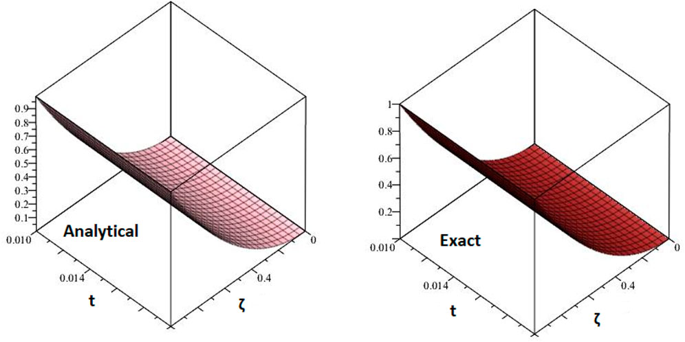
FIGURE 1. 3D plots for the exact and analytical solution at γ =1 for Example 1.

FIGURE 2

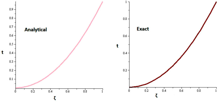
FIGURE 2. 2D plots for the exact and analytical solution at γ =1 for Example 1.

FIGURE 3

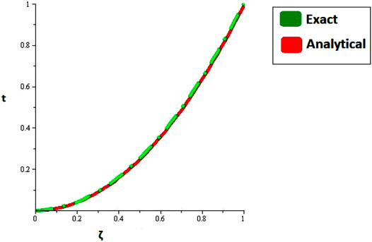
FIGURE 3. Comparison for the exact and analytical solution at γ =1 for Example 1.

FIGURE 4

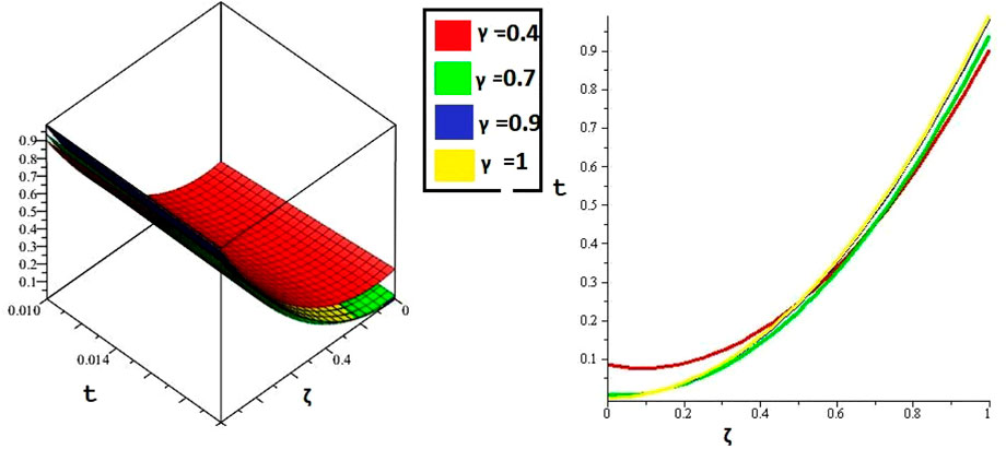
FIGURE 4. 3D and 2D plots for the ADM solution at different values of γ for Example 1.

FIGURE 5

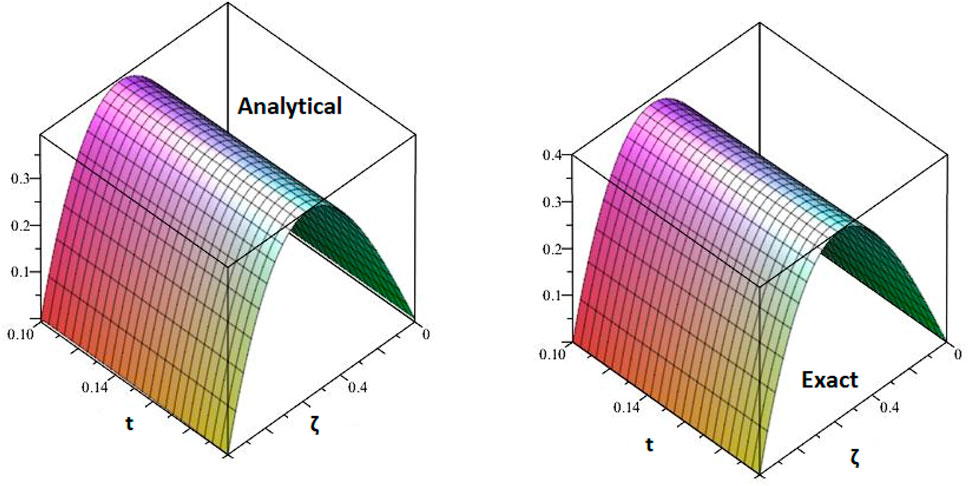
FIGURE 5. 3D plots for the exact and analytical solution at γ =1 for Example 2.

FIGURE 6

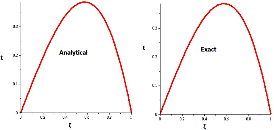
FIGURE 6. 2D plots for the exact and analytical solution at γ =1 for Example 2.

FIGURE 7

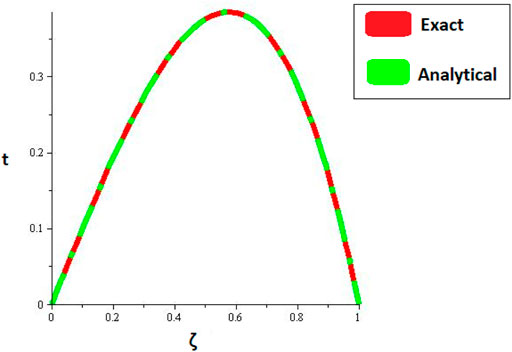
FIGURE 7. Comparison for the exact and analytical solution at γ =1 for Example 2.

FIGURE 8

FIGURE 8. 3D and 2D plots for the ADM solution at different values of γ =1 for Example 2.

FIGURE 9

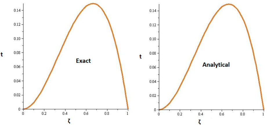
FIGURE 9. 3D plots for the exact and analytical solution at γ =1 for Example 3.

FIGURE 10

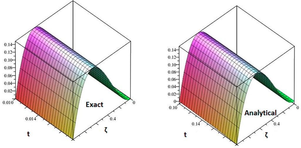
FIGURE 10. 2D plots for the exact and analytical solution at γ =1 for Example 3.

FIGURE 11

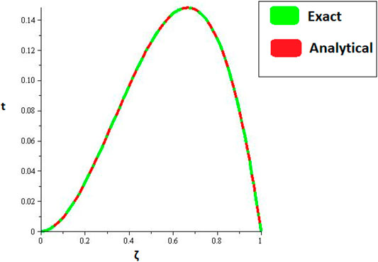
FIGURE 11. Comparison for the exact and analytical solution at γ =1 for Example 3.

FIGURE 12

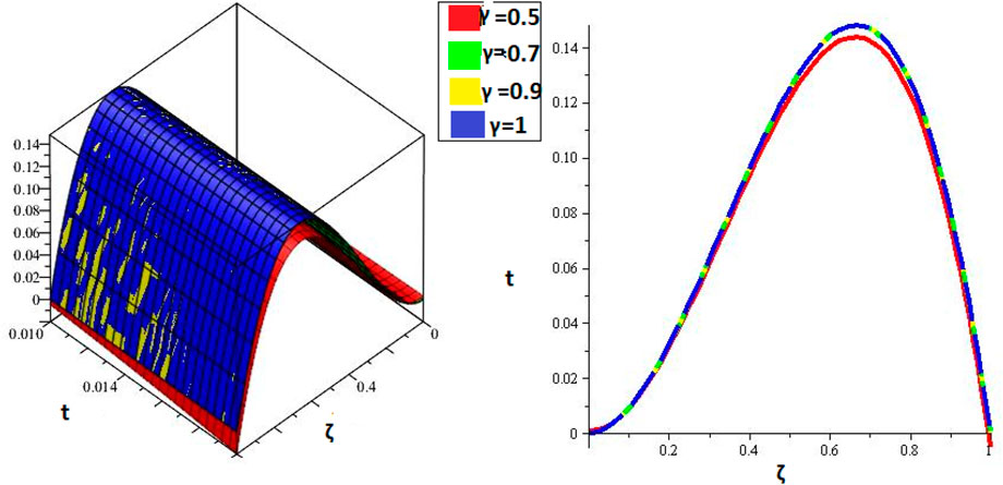
FIGURE 12. 3D and 2D plots for the ADM solution at different values of γ for Example 3.

FIGURE 13

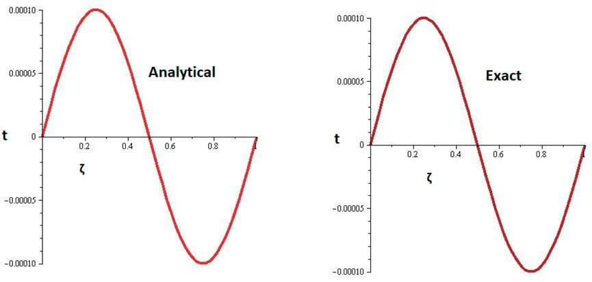
FIGURE 13. 3D plots for the exact and analytical solution at γ =1 for Example 4

FIGURE 14

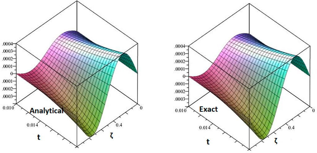
FIGURE 14. 2D plots for the exact and analytical solution at γ =1 for Example 4

FIGURE 15

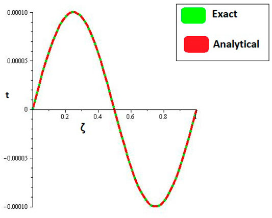
FIGURE 15. Comparison for the exact and analytical solution at γ =1 for Example 4.

FIGURE 16

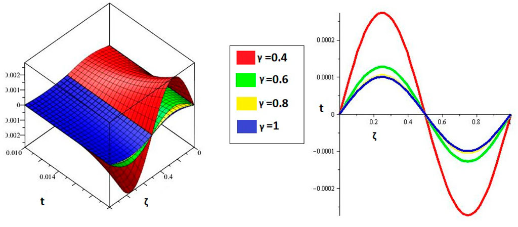
FIGURE 16. 3D and 2D plots for the ADM solution at different values of γ for Example 4.

7 Conclusion

In many situations, the analytical solutions of fractional partial differential equations with boundary conditions are very difficult to investigate. Here, a very useful and successful attempt is made to determine the solution of fractional convection–diffusion equations with variable coefficients along with the initial–boundary conditions. The simulations for the given problems are derived and applied it for the solutions of some numerical examples. The fractional-order solutions are obtained in a very sophisticated manner. The solution graphs are plotted with higher accuracy for both fractional and integer orders of the problems. It is shown that the solution sequence of fractional order problems is convergent towards the integer-order solutions. Moreover, it is investigated that the present method has a unique capability to solve fractional partial differential equations with variable coefficients with initial and boundary conditions. In the light of the above varieties and features, the proposed technique can be extended to solve other problems with higher accuracy.

Data Availability Statement

The original contributions presented in the study are included in the article/supplementary material, and further inquiries can be directed to the corresponding author.

Author Contributions

HK supervision, PK funding, Hajira methodology, QK Investigation, FT Project Administrator, KS Funding, ID draft writing.

Funding

The authors acknowledge the financial support provided by the Center of Excellence in Theoretical and Computational Science (TaCS-CoE), KMUTT. This research project is supported by Thailand Science Research and Innovation (TSRI) Basic Research Fund: Fiscal year 2022 under project number FRB650048/0164.

Conflict of Interest

The authors declare that the research was conducted in the absence of any commercial or financial relationships that could be construed as a potential conflict of interest.

Publisher’s Note

All claims expressed in this article are solely those of the authors and do not necessarily represent those of their affiliated organizations, or those of the publisher, the editors, and the reviewers. Any product that may be evaluated in this article, or claim that may be made by its manufacturer, is not guaranteed or endorsed by the publisher.

Acknowledgments

Researchers Supporting Project number (RSP-2021/401), King Saud University, Riyadh, Saudi Arabia.

References

1. Gorenflo R, Mainardi F. Fractional Calculus. In: Fractals and Fractional Calculus in Continuum Mechanics. Vienna: Springer (1997). p. 223–76. doi:10.1007/978-3-7091-2664-6_5

CrossRef Full Text | Google Scholar

2. Zaslavsky GM, Zaslavskij GM. Hamiltonian Chaos and Fractional Dynamics. Oxford, England: Oxford University Press on Demand (2005).

Google Scholar

3. Hilfer R. Applications of Fractional Calculus in Physics. World Scientific (2000).

Google Scholar

4. Podlubny I. Fractional Differential Equations: An Introduction to Fractional Derivatives, Fractional Differential Equations, to Methods of Their Solution and Some of Their Applications. Amsterdam, Netherlands: Elsevier (1998).

Google Scholar

5. Meerschaert MM, Scalas E. Coupled Continuous Time Random Walks in Finance. Physica A: Stat Mech its Appl (2006) 370(1):114–8. doi:10.1016/j.physa.2006.04.034

CrossRef Full Text | Google Scholar

6. Chauhan NS. A New Approach for Solving Fractional RL Circuit Model through Quadratic Legendre Multi-Wavelets. Int J Math Phys (2018) 1:1–9. doi:10.18063/ijmp.v1i1.724

CrossRef Full Text | Google Scholar

7. Mainardi F. Fractional Calculus: Some Basic Problems in Continuum and Statistical Mechanics. arXiv preprint arXiv:1201.0863 (2012).

Google Scholar

8. Bohannan GW. Analog Fractional Order Controller in Temperature and Motor Control Applications. J Vibration Control (2008) 14(9-10):1487–98. doi:10.1177/1077546307087435

CrossRef Full Text | Google Scholar

9. Goswami A, Singh J, Kumar D. An Efficient Analytical Approach for Fractional Equal Width Equations Describing Hydro-Magnetic Waves in Cold Plasma. Physica A: Stat Mech its Appl (2019) 524:563–75. doi:10.1016/j.physa.2019.04.058

CrossRef Full Text | Google Scholar

10. Bai J, Feng X-C. Fractional-order Anisotropic Diffusion for Image Denoising. IEEE Trans Image Process (2007) 16(10):2492–502. doi:10.1109/tip.2007.904971

PubMed Abstract | CrossRef Full Text | Google Scholar

11. Baleanu D, Sadat Sajjadi S, Jajarmi A, Asad JH. New Features of the Fractional Euler-Lagrange Equations for a Physical System within Non-singular Derivative Operator. Eur Phys J Plus (2019) 134(4):181. doi:10.1140/epjp/i2019-12561-x

CrossRef Full Text | Google Scholar

12. Jumarie G. Fractional Hamilton-Jacobi Equation for the Optimal Control of Nonrandom Fractional Dynamics with Fractional Cost Function. J Appl Mathematics Comput (2007) 23(1):215–28. doi:10.1007/bf02831970

CrossRef Full Text | Google Scholar

13. Frederico GSF, Torres DFM. Fractional Conservation Laws in Optimal Control Theory. Nonlinear Dyn (2008) 53(3):215–22. doi:10.1007/s11071-007-9309-z

CrossRef Full Text | Google Scholar

14. Wu X, Lai D, Lu H. Generalized Synchronization of the Fractional-Order Chaos in Weighted Complex Dynamical Networks with Nonidentical Nodes. Nonlinear Dyn (2012) 69(1):667–83. doi:10.1007/s11071-011-0295-9

CrossRef Full Text | Google Scholar

15. Singh J, Kumar D, Baleanu D. On the Analysis of Fractional Diabetes Model with Exponential Law. Adv Difference Equations (2018) 2018(1):1–15. doi:10.1186/s13662-018-1680-1

CrossRef Full Text | Google Scholar

16. Gao W, Veeresha P, Prakasha DG, Baskonus HM. Novel Dynamic Structures of 2019-nCoV with Nonlocal Operator via Powerful Computational Technique. Biology (Basel) (2020) 9(5):107. doi:10.3390/biology9050107

PubMed Abstract | CrossRef Full Text | Google Scholar

17. Podlubny I, Chechkin A, Skovranek T, Chen Y, Vinagre Jara BM. Matrix Approach to Discrete Fractional Calculus II: Partial Fractional Differential Equations. J Comput Phys (2009) 228(8):3137–53. doi:10.1016/j.jcp.2009.01.014

CrossRef Full Text | Google Scholar

18. Miller KS, Ross B. An Introduction to the Fractional Calculus and Fractional Differential Equations. Hoboken, New Jersey: Wiley (1993).

Google Scholar

19. Oldham K, Spanier J. The Fractional Calculus Theory and Applications of Differentiation and Integration to Arbitrary Order. Amsterdam, Netherlands: Elsevier (1974).

Google Scholar

20. Kilbas AA, Trujillo JJ. Differential Equations of Fractional Order: Methods Results and Problem—I. Applicable Anal (2001) 78(1-2):153–92. doi:10.1080/00036810108840931

CrossRef Full Text | Google Scholar

21. Benchohra M, Hamani S, Ntouyas S. Boundary Value Problems for Differential Equations with Fractional Order and Nonlocal Conditions. Nonlinear Anal Theor Methods Appl (2009) 71(7-8):2391–6. doi:10.1016/j.na.2009.01.073

CrossRef Full Text | Google Scholar

22. Ahmad WM, El-Khazali R. Fractional-order Dynamical Models of Love. Chaos, Solitons & Fractals (2007) 33(4):1367–75. doi:10.1016/j.chaos.2006.01.098

CrossRef Full Text | Google Scholar

23. Singh J, Kumar D, Swroop R. Numerical Solution of Time- and Space-Fractional Coupled Burgers' Equations via Homotopy Algorithm. Alexandria Eng J (2016) 55(2):1753–63. doi:10.1016/j.aej.2016.03.028

CrossRef Full Text | Google Scholar

24. Gupta AK, Ray SS. The Comparison of Two Reliable Methods for Accurate Solution of Time-Fractional Kaup-Kupershmidt Equation Arising in Capillary Gravity Waves. Math Meth Appl Sci (2016) 39(3):583–92. doi:10.1002/mma.3503

CrossRef Full Text | Google Scholar

25. Saha Ray S, Gupta AK. Numerical Solution of Fractional Partial Differential Equation of Parabolic Type with Dirichlet Boundary Conditions Using Two-Dimensional Legendre Wavelets Method. J Comput Nonlinear Dyn (2016) 11(1):1–9. doi:10.1115/1.4028984

CrossRef Full Text | Google Scholar

26. Chen Y, Sun Y, Liu L. Numerical Solution of Fractional Partial Differential Equations with Variable Coefficients Using Generalized Fractional-Order Legendre Functions. Appl Mathematics Comput (2014) 244:847–58. doi:10.1016/j.amc.2014.07.050

CrossRef Full Text | Google Scholar

27. Guo S, Mei L, Li Y, Sun Y. The Improved Fractional Sub-equation Method and its Applications to the Space-Time Fractional Differential Equations in Fluid Mechanics. Phys Lett A (2012) 376(4):407–11. doi:10.1016/j.physleta.2011.10.056

CrossRef Full Text | Google Scholar

28. Jaradat I, Alquran M, Al-Khaled K. An Analytical Study of Physical Models with Inherited Temporal and Spatial Memory. Eur Phys J Plus (2018) 133(4):162–9. doi:10.1140/epjp/i2018-12007-1

CrossRef Full Text | Google Scholar

29. Srivastava HM, Shah R, Khan H, Arif M. Some Analytical and Numerical Investigation of a Family of Fractional‐order Helmholtz Equations in Two Space Dimensions. Math Meth Appl Sci (2020) 43(1):199–212. doi:10.1002/mma.5846

CrossRef Full Text | Google Scholar

30. Yuanlu LI. Solving a Nonlinear Fractional Differential Equation Using Chebyshev Wavelets. Commun Nonlinear Sci Numer Simulation (2010) 15(9):2284–92. doi:10.1016/j.cnsns.2009.09.020

CrossRef Full Text | Google Scholar

31. Ali EJ. A New Technique of Initial Boundary Value Problems Using Adomian Decomposition Method. Int Math Forum (2012) 7(17):799–814.

Google Scholar

32. Dhaigude DB, Birajdar GA. Numerical Solution of Fractional Partial Differential Equations by Discrete Adomian Decomposition Method. Adv Appl Mathematics Mech (2014) 6(1):107–19. doi:10.4208/aamm.12-m12105

CrossRef Full Text | Google Scholar

33. Shah R, Farooq U, Khan H, Baleanu D, Kumam P, Arif M. Fractional View Analysis of Third Order Kortewege-De Vries Equations, Using a New Analytical Technique. Front Phys (2020) 7:244. doi:10.3389/fphy.2019.00244

CrossRef Full Text | Google Scholar

34. Kadem A, Baleanu D. Analytical Method Based on Walsh Function Combined with Orthogonal Polynomial for Fractional Transport Equation. Commun Nonlinear Sci Numer Simulation (2010) 15(3):491–501. doi:10.1016/j.cnsns.2009.05.024

CrossRef Full Text | Google Scholar

35. Kadem A. The Fractional Transport Equation: an Analytical Solution and a Spectral Approximation by Chebyshev Polynomials. Appl Sci (2009) 11:78–90.

Google Scholar

36. Ara A, Khan NA, Razzaq OA, Hameed T, Raja MAZ. Wavelets Optimization Method for Evaluation of Fractional Partial Differential Equations: an Application to Financial Modelling. Adv Difference Equations (2018) 2018(1):1–13. doi:10.1186/s13662-017-1461-2

CrossRef Full Text | Google Scholar

37. Fabian AL, Kohl R, Biswas A. Perturbation of Topological Solitons Due to Sine-Gordon Equation and its Type. Commun Nonlinear Sci Numer Simulation (2009) 14(4):1227–44. doi:10.1016/j.cnsns.2008.01.013

CrossRef Full Text | Google Scholar

38. Ma W-X, Zhu Z. Solving the (3+1)-dimensional Generalized KP and BKP Equations by the Multiple Exp-Function Algorithm. Appl Mathematics Comput (2012) 218(24):11871–9. doi:10.1016/j.amc.2012.05.049

CrossRef Full Text | Google Scholar

39. Ma W-X. Bilinear Equations, Bell Polynomials and Linear Superposition Principle. J Phys Conf Ser.IOP Publishing (2013) 411(No. 1):012021. doi:10.1088/1742-6596/411/1/012021

CrossRef Full Text | Google Scholar

40. Xu J, Khan H, Khan H, Shah R, Alderremy AA, Aly S, et al. The Analytical Analysis of Nonlinear Fractional-Order Dynamical Models. AIMS Mathematics (2021) 6(6):6201–19. doi:10.3934/math.2021364

CrossRef Full Text | Google Scholar

41. Eltayeb H, Abdalla Y, Bachar I, Khabir M. Fractional Telegraph Equation and its Solution by Natural Transform Decomposition Method. Symmetry (2019) 11(3):334. doi:10.3390/sym11030334

CrossRef Full Text | Google Scholar

42. Chen Y, Wu Y, Cui Y, Wang Z, Jin D. Wavelet Method for a Class of Fractional Convection-Diffusion Equation with Variable Coefficients. J Comput Sci (2010) 1(3):146–9. doi:10.1016/j.jocs.2010.07.001

CrossRef Full Text | Google Scholar

43. Atangana A, Doungmo-Goufo EF. Solution of Diffusion Equation with Local Derivative with New Parameter. Therm Sci (2015) 19(Suppl. 1):231–8. doi:10.2298/tsci15s1s31a

CrossRef Full Text | Google Scholar

44. Wazwaz A-M, El-Sayed SM. A New Modification of the Adomian Decomposition Method for Linear and Nonlinear Operators. Appl Mathematics Comput (2001) 122(3):393–405. doi:10.1016/s0096-3003(00)00060-6

CrossRef Full Text | Google Scholar

45. Hu Y, Luo Y, Lu Z. Analytical Solution of the Linear Fractional Differential Equation by Adomian Decomposition Method. J Comput Appl Mathematics (2008) 215(1):220–9. doi:10.1016/j.cam.2007.04.005

CrossRef Full Text | Google Scholar

46. Saha Ray S, Bera RK. An Approximate Solution of a Nonlinear Fractional Differential Equation by Adomian Decomposition Method. Appl Mathematics Comput (2005) 167(1):561–71. doi:10.1016/j.amc.2004.07.020

CrossRef Full Text | Google Scholar

47. Hashim I. Adomian Decomposition Method for Solving BVPs for Fourth-Order Integro-Differential Equations. J Comput Appl Mathematics (2006) 193(2):658–64. doi:10.1016/j.cam.2005.05.034

CrossRef Full Text | Google Scholar

48. Duan J-S, Rach R. A New Modification of the Adomian Decomposition Method for Solving Boundary Value Problems for Higher Order Nonlinear Differential Equations. Appl Mathematics Comput (2011) 218(8):4090–118. doi:10.1016/j.amc.2011.09.037

CrossRef Full Text | Google Scholar

49. Song L, Wang W. A New Improved Adomian Decomposition Method and its Application to Fractional Differential Equations. Appl Math Model (2013) 37(3):1590–8. doi:10.1016/j.apm.2012.03.016

CrossRef Full Text | Google Scholar

50. Wu GC. Adomian Decomposition Method for Non-smooth Initial Value Problems. Math Computer Model (2011) 54(9-10):2104–8. doi:10.1016/j.mcm.2011.05.018

CrossRef Full Text | Google Scholar

51. Almazmumy M, Hendi FA, Bakodah HO, Alzumi H. Recent Modifications of Adomian Decomposition Method for Initial Value Problem in Ordinary Differential Equations. Ajcm (2012) 02:228–34. doi:10.4236/ajcm.2012.23030

CrossRef Full Text | Google Scholar

52. Patel T, Meher R. Thermal Analysis of Porous Fin with Uniform Magnetic Field Using Adomian Decomposition Sumudu Transform Method. Nonlinear Eng (2017) 6(3):191–200. doi:10.1515/nleng-2017-0021

CrossRef Full Text | Google Scholar

53. Patel T, Meher R. Adomian Decomposition Sumudu Transform Method for Convective Fin with Temperature-dependent Internal Heat Generation and thermal Conductivity of Fractional Order Energy Balance Equation. Int J Appl Comput Math (2017) 3(3):1879–95. doi:10.1007/s40819-016-0208-1

CrossRef Full Text | Google Scholar

54. Patel HS, Patel T. Applications of Fractional Reduced Differential Transform Method for Solving the Generalized Fractional-Order Fitzhugh–Nagumo Equation. Int J Appl Comput Mathematics (2021) 7(5):1–15. doi:10.1007/s40819-021-01130-2

CrossRef Full Text | Google Scholar

55. Patel H, Patel T, Pandit D. An Efficient Technique for Solving Fractional-Order Diffusion Equations Arising in Oil Pollution. J Ocean Eng Sci (2022) 1–9. doi:10.1016/j.joes.2022.01.004

CrossRef Full Text | Google Scholar

56. Turkyilmazoglu M. Accelerating the Convergence of Adomian Decomposition Method (ADM). J Comput Sci (2019) 31:54–9. doi:10.1016/j.jocs.2018.12.014

CrossRef Full Text | Google Scholar

57. Turkyilmazoglu M. Nonlinear Problems via a Convergence Accelerated Decomposition Method of Adomian. Computer Model Eng Sci (2021) 127:1–22. doi:10.32604/cmes.2021.012595

CrossRef Full Text | Google Scholar

58. Fatoorehchi H, Rach R, Sakhaeinia H. Explicit Frost-Kalkwarf Type Equations for Calculation of Vapour Pressure of Liquids from Triple to Critical point by the Adomian Decomposition Method. Can J Chem Eng (2017) 95(11):2199–208. doi:10.1002/cjce.22853

CrossRef Full Text | Google Scholar

59. Elaf JA. Modified Treatment of Initial Boundary Value Problems for One Dimensional Heat-like and Wave-like Equations Using Adomian Decomposition Method. basrah J Sci (2012) 30:86–105.

Google Scholar

60. Ali EJ. New Treatment of Initial Boundary Problems for Fourth-Order Parabolic Partial Differential Equations Using Variational Iteration Method. Int J Contemp Math Sci (2011) 6(48):2367–76.

Google Scholar

61. Aminataei A, Hosseini SS. The Comparison of the Stability of Adomian Decomposition Method with Numerical Methods of Equation Solution. Appl Math Comput (2007) 186(1):665–9. doi:10.1016/j.amc.2006.08.011

CrossRef Full Text | Google Scholar

62. Abdelrazec A, Pelinovsky D. Convergence of the Adomian Decomposition Method for Initial-Value Problems. Numer Methods Partial Differential Eq (2011) 27(4):749–66. doi:10.1002/num.20549

CrossRef Full Text | Google Scholar

63. Izadkhah MM, Saberi-Nadjafi J. Gegenbauer Spectral Method for Time-Fractional Convection-Diffusion Equations with Variable Coefficients. Math Meth Appl Sci (2015) 38(15):3183–94. doi:10.1002/mma.3289

CrossRef Full Text | Google Scholar

64. Saadatmandi A, Dehghan M, Azizi M-R. The Sinc-Legendre Collocation Method for a Class of Fractional Convection-Diffusion Equations with Variable Coefficients. Commun Nonlinear Sci Numer Simulation (2012) 17(11):4125–36. doi:10.1016/j.cnsns.2012.03.003

CrossRef Full Text | Google Scholar

65. Chen Y, Yi M, Chen C, Yu C. Bernstein Polynomials Method for Fractional Convection-Diffusion Equation with Variable Coefficients. Computer Model Eng Sciences(CMES) (2012) 83(6):639–53.

Google Scholar

66. Irandoust-pakchin S, Dehghan M, Abdi-mazraeh S, Lakestani M. Numerical Solution for a Class of Fractional Convection-Diffusion Equations Using the Flatlet Oblique Multiwavelets. J Vibration Control (2014) 20(6):913–24. doi:10.1177/1077546312470473

CrossRef Full Text | Google Scholar

67. Akinfe TK, Loyinmi AC. A Solitary Wave Solution to the Generalized Burgers-Fisher's Equation Using an Improved Differential Transform Method: A Hybrid Scheme Approach. Heliyon (2021) 7(5):e07001. doi:10.1016/j.heliyon.2021.e07001

PubMed Abstract | CrossRef Full Text | Google Scholar

68. Uddin M, Haq S. RBFs Approximation Method for Time Fractional Partial Differential Equations. Commun Nonlinear Sci Numer Simulation (2011) 16(11):4208–14. doi:10.1016/j.cnsns.2011.03.021

CrossRef Full Text | Google Scholar

69. Luo W-H, Huang T-Z, Wu G-C, Gu X-M. Quadratic Spline Collocation Method for the Time Fractional Subdiffusion Equation. Appl Mathematics Comput (2016) 276:252–65. doi:10.1016/j.amc.2015.12.020

CrossRef Full Text | Google Scholar

70. Pirkhedri A, Javadi HHS. Solving the Time-Fractional Diffusion Equation via Sinc-Haar Collocation Method. Appl Mathematics Comput (2015) 257:317–26. doi:10.1016/j.amc.2014.12.110

CrossRef Full Text | Google Scholar

71. Adomian G. Solving Frontier Problems of Physics: the Decomposition Method, with a Preface by Yves Cherruault. Fundam Theories Phys (1994) 1:1–42.

Google Scholar

72. Angulo JM, Ruiz-Medina MD, Anh VV, Grecksch W. Fractional Diffusion and Fractional Heat Equation. Adv Appl Probab (2000) 32:1077–99. doi:10.1239/aap/1013540349

CrossRef Full Text | Google Scholar

73. Shah R, Khan H, Baleanu D, Kumam P, Arif M. A Novel Method for the Analytical Solution of Fractional Zakharov–Kuznetsov Equations. Adv Difference Equations (2019) 2019(1):1–14. doi:10.1186/s13662-019-2441-5

CrossRef Full Text | Google Scholar

74. Shah R, Khan H, Kumam P, Arif M, Baleanu D. Natural Transform Decomposition Method for Solving Fractional-Order Partial Differential Equations with Proportional Delay. Mathematics (2019) 7(6):532. doi:10.3390/math7060532

CrossRef Full Text | Google Scholar

75. Duan J-S. Convenient Analytic Recurrence Algorithms for the Adomian Polynomials. Appl Mathematics Comput (2011) 217(13):6337–48. doi:10.1016/j.amc.2011.01.007

CrossRef Full Text | Google Scholar

76. Zhu X, Nie Y. On a Collocation Method for the Time-Fractional Convection-Diffusion Equation with Variable Coefficients. arXiv preprint arXiv:1604.02112 (2016).

Google Scholar

77. Zhou F, Xu X. The Third Kind Chebyshev Wavelets Collocation Method for Solving the Time-Fractional Convection Diffusion Equations with Variable Coefficients. Appl Mathematics Comput (2016) 280:11–29. doi:10.1016/j.amc.2016.01.029

CrossRef Full Text | Google Scholar