The Efficient Techniques for Non-Linear Fractional View Analysis of the KdV Equation

The solutions to fractional differentials equations are very difficult to investigate. In particular, the solutions of fractional partial differential equations are challenging tasks for mathematicians. In the present article, an extension to this idea is presented to obtain the solutions of non-linear fractional Korteweg–de Vries equations. The solutions comparison of the proposed problems is done via two analytical procedures, which are known as the Residual power series method (RPSM) and q-HATM, respectively. The graphical and tabular analysis are presented to show the reliability and competency of the suggested techniques. The comparison has shown the greater contact between exact, RPSM, and q-HATM solutions. The fractional solutions are in good control and provide many important dynamics of the given problems.

1 Introduction

Fractional Calculus literature dates back to 1,695 and considered to be as old as classical calculus. L’Hospital was the first to write a letter to Leibnitz about the concept of the time-fractional derivative, and progress in that direction has been gradual since that time. Later on N. H. Abel, L. Euler, J. Liouvilles, H. Holmgren, J. B. J. Fourier, A. K. Gruwald, P. S. Laplace, B. Riemann, E. R. Love, A. V. Letnikov, A. Krug, J. Hadamard, S. Pincherle, H. Weyl, O. Heaviside are among the few Nobel laureates in mathematics till the 20th century. Other Mathematicians such as H. Laurent, G.H. Hardy, and J. E. Liitlewood, as well as P. Levy, A. Marchand, H. T. Davis, A. Zygmund, A. Erde’lyi, H. Kober, D. V. widder, and M. Riesz, have contributed a lot towards FC. After 1930, there was infrequent additional research in this subject.

FC is a substitute calculus that may be used to appropriately design a variety of phenomena such as Optics [1], Hepatitis B Virus [3], Tuberculosis [4], Air foil [5], modelling of Earth quack nonlinear oscillation [6], Propagation of Spherical Waves [7], the fluid traffic [8], Chaos theory [9], Finance [11], economics [12], Zener [10], Cancer chemotherapy [13], Electrodynamics [14], heat transfer model [15], the fractional nonlinear space-time nuclear model [16], traffic flow model [17], Poisson-NerstPlanck diffusion [18], Pine wilt disease [19], Diabetes [20], fractional COVID-19 Model [2], biomedical and biological [21] and other applications in various branches of research [22–24]. Fractional differential and integral equations have been found to be the most desired tools for appropriately designing numerous physical processes. The polymers model with rheological characteristics, is the most important design that has been represented by FDEs. some others advanced development of FDEs includes bio tissues, nuclear mechanics, ractional diffusion, involuntary vibrations and thermo-elasticity [25–31].

Many mathematicians have made their efforts to develop or implement numerical and analytical techniques for the solutions of non-linear fractional partial differential equations (FPDEs). In this context, Hassan et al. have presented the solutions of some non-linear FPDEs and their systems in [32–35]. Many Other important and efficient techniques that have been implemented to solve FPDEs and their systems are Iterative Laplace transform method [38], optimal homotopy asymptotic method (OHAM) [39], extended direct algebraic method (EDAM) [49], Adomian decomposition method (ADM) [40, 41], Natural transform method [42], the Finite difference method (FDM) [43], the (G/Ǵ)-expansion method [48], the Homotopy perturbation transform technique along with transformation (HPTM) [44, 45, 47], standard reductive perturbation method [50], the Haar wavelet method (HWM) [51, 52], spectral collocation method (SCM) [46], the Variational iteration procedure with transformation (VITM) [58] and the differential transform method (DTM) [53–55]. In similar way, the novel techniques have been used for the solutions of Korteweg–de Vries equation and time-fractional Drinfeld–Sokolov–Wilson system and can be cited in [56, 57].

In this article, We are working with two efficient techniques, namely residual power series method (RPSM) and q-homotopy analysis transform method (q-HATM) to obtain the analytical solutions of Korteweg–de Vries equation (KdV) equations. The goal of the present research is to use q-HATM and RPSM to visualise the solutions to the KdV equations. The RPSM has a simple and fluent implementation in both strongly linear and nonlinear IVPs. RPSM [59] is used to construct power series solutions with the exception of perturbation and linearization. For an approximate analytical solution, the suggested approach uses a polynomial. The suggested approach is dominant over the Taylor series method because it allows to control large-scale computing. RPSM is used for systematically investigating the coefficients of a series form solutions. A fundamental advantage of RPSM is that it can be applied to other FPDEs and system of FPDEs. Another method which is known as q-HATM [36, 37] is the result of combining HAM and LTM when $q\in [0,\frac{1}{n}]$. The benefit of q-HATM is that it adds two strong computational approaches to solve FPDEs. The goal of this method is to create a precise function that can be solved using homotopy polynomials. The illustrative examples demonstrate the viability of q-HATM. The proposed approaches are similar to implement for multi-dimensional non-integer physical problems.

In this research paper, the solutions of various FPDEs related to KdV equations are investigated by using the proposed analytical techniques, q-HAM and RPSM, at the same time. The suggested techniques have different procedure to obtain the solutions of fractional KdV equations. The obtained results of the two innovative techniques are compared to one another as well as with the exact solutions to the problems. The obtained results are displayed by using graphs and tables. The absolute errors at different fractional order are calculated and have shown the greater accuracy of the proposed methods. The RPSM procedure is simple and has a direct implementation to the targeted problems. Moreover, the linearity of the problems is handled in a very sophisticated manner as compare to other analytical procedures. The exact and approximate solutions for both techniques are very closed to the exact solutions of the given KdV equations. The fractional solutions are very convergent towards the integer order solutions and obey the higher efficiency of the present techniques. This paper is structured as follows: Section 2 represent some basic definition. Section 3 is the methodology while in Section 4 some numerical results are compared by using two powerful methods. Section 5 is the conclusion section. References are present at the end of the paper.

2 Basic Definitions

In this section we will discuss some important definitions.

2.1 Caputo Operator

For function $f(\mathfrak{I})$, the Caputo derivative of order δ is define as [60, 61].

${\mathfrak{D}}_{\mathfrak{I}}^{\delta }f\left(\mathfrak{I}\right)=\left\{\begin{array}{cc}\frac{d^{n}f\left(\mathfrak{I}\right)}{d{\mathfrak{I}}^n},\hfill & \delta =n\in N,\hfill \\ \frac{1}{\mathrm{\Gamma }\left(n-\delta \right)}{\int }_0^{\mathfrak{I}}{\left(\mathfrak{I}-\varsigma \right)}^{n-\delta -1}{f}^{\left(n\right)}\left(\varsigma \right)d\varsigma ,\hfill & n<\delta <n+1,n\in N.\hfill \end{array}\right.$

2.2 Definition

An expansion of power series (PS) at point $\mathfrak{I}={\mathfrak{I}}_0$ is known as fractional PS and is given by [63].

$\begin{array}{ll}\hfill \sum _{\text{n}=0}^{\infty }{a}_n{\left(\mathfrak{I}-{\mathfrak{I}}_0\right)}^{n\delta }& =a_0+a_1{\left(\mathfrak{I}-{\mathfrak{I}}_0\right)}^{\delta }+a_2{\left(\mathfrak{I}-{\mathfrak{I}}_0\right)}^{2\delta }+\cdots ,\hfill \\ \hfill \&\\ \hfill \sum _{n=0}^{\infty }{f}_n\left(\varsigma \right){\left(\mathfrak{I}-{\mathfrak{I}}_0\right)}^{n\delta }& =f_0\left(\varsigma \right)+f_1\left(\varsigma \right){\left(\mathfrak{I}-{\mathfrak{I}}_0\right)}^{\delta }+f_2\left(\varsigma \right){\left(\mathfrak{I}-{\mathfrak{I}}_0\right)}^{2\delta }+\cdots ,n-1<\delta \le n,\mathfrak{I}\ge {\mathfrak{I}}_0,\hfill \end{array}$

Note: FPS can be expanded at point ${\mathfrak{I}}_0$ as

$y\left(\varsigma ,\mathfrak{I}\right)=\sum _{n=0}^{\infty }\frac{{\mathfrak{D}}_{\mathfrak{I}}^{n\delta }y\left(\varsigma ,{\mathfrak{I}}_0\right)}{\mathrm{\Gamma }\left(n\delta +1\right)}{\left(\mathfrak{I}-{\mathfrak{I}}_0\right)}^{n\delta },0\le n-1<\delta \le m,\varsigma \in I,{\mathfrak{I}}_0\le \mathfrak{I}<{\mathfrak{I}}_0+\mathfrak{R},$

which is the Taylor’s series expansion form.

2.3 Laplace Transform

The LT for continuous function $\mathfrak{g}(\mathfrak{I})$ is defined as [62].

$G\left(s\right)=\mathcal{L}\left[\mathfrak{g}\left(\mathfrak{I}\right)\right]={\int }_0^{\infty }{e}^{-s\mathfrak{I}}\mathfrak{g}\left(\mathfrak{I}\right)d\mathfrak{I},$

here G(s) is the LT for the function $\mathfrak{g}(\mathfrak{I})$.

2.4 Definition

The LT $\mathcal{L}[y(\varsigma ,\mathfrak{I})]$ of Caputo fractional derivative is given by [62].

$\mathcal{L}\left[{\mathfrak{D}}_{\mathfrak{I}}^{n\delta }y\left(\varsigma ,\mathfrak{I}\right)\right]=s^{n\delta }\mathcal{L}\left[y\left(\varsigma ,\mathfrak{I}\right)\right]-\sum _{k=0}^{n-1}{s}^{n\delta -k-1}{y}^k\left(\varsigma ,0\right),n-1<n\delta \le n.(1)$

3 Methodology of RPSM and q-HATM for FPDEs

Consider a generalized non-linear FPDEs,

${\mathfrak{D}}_{\mathfrak{I}}^{\delta }y\left(\varsigma ,\mathfrak{I}\right)=N\left(y\left(\varsigma ,\mathfrak{I}\right)\right)+R\left(y\left(\varsigma ,\mathfrak{I}\right)\right),n-1<\delta \le n,\mathfrak{I}>0,(2)$

with initial condition,

$y\left(\varsigma ,0\right)=f\left(\varsigma \right),(3)$

where ${\mathfrak{D}}_{\mathfrak{I}}^{\delta }$ is the Caputo type fractional derivative, R is linear and N are non-linear terms.

3.1 RPSM Procedure

The procedure of RPSM [64] for the solution of Eq. 2 is given below.

Let

$y\left(\varsigma ,\mathfrak{I}\right)=\sum _{n=0}^{\infty }{f}_n\left(\varsigma \right)\frac{{\mathfrak{I}}^{n\delta }}{\mathrm{\Gamma }\left(1+n\delta \right)},0<\delta \le 1,-\infty <\varsigma <\infty ,0\le \mathfrak{I}<R,(4)$

the kth truncated series for $y(\varsigma ,\mathfrak{I})$ is given as

$y_k\left(\varsigma ,\mathfrak{I}\right)=\sum _{n=0}^k{f}_n\left(\varsigma \right)\frac{{\mathfrak{I}}^{n\delta }}{\mathrm{\Gamma }\left(1+n\delta \right)},(5)$

for k = 0 Eq. 5, become as

$y_0\left(\varsigma ,\mathfrak{I}\right)=y\left(\varsigma ,0\right)=f\left(\varsigma \right),(6)$

further Eq. 5, implies that,

$y_k\left(\varsigma ,\mathfrak{I}\right)=f\left(\varsigma \right)+\sum _{n=1}^k{f}_n\left(\varsigma \right)\frac{{\mathfrak{I}}^{n\delta }}{\mathrm{\Gamma }\left(1+n\delta \right)},k=\mathrm{1,2},\dots ,(7)$

for Eq. 2, residual function is presented as

$Re{s}_y\left(\varsigma ,\mathfrak{I}\right)={\mathfrak{D}}_{\mathfrak{I}}^{\delta }y\left(\varsigma ,\mathfrak{I}\right)-N\left(y\left(\varsigma ,\mathfrak{I}\right)\right)-R\left(y\left(\varsigma ,\mathfrak{I}\right)\right),(8)$

so, the kth residual function becomes

$Re{s}_{y,k}\left(\varsigma ,\mathfrak{I}\right)={\mathfrak{D}}_{\mathfrak{I}}^{\delta }{y}_k\left(\varsigma ,\mathfrak{I}\right)-N\left(y_k\left(\varsigma ,\mathfrak{I}\right)\right)-R\left(y_k\left(\varsigma ,\mathfrak{I}\right)\right).(9)$

As in [65, 66], it show that $Res(\varsigma ,\mathfrak{I})=0$ and ${\lim }_{n\to \infty }Re{s}_k(\varsigma ,\mathfrak{I})=Res(\varsigma ,\mathfrak{I})$. Therefore, ${\mathfrak{D}}_{\mathfrak{I}}^{n\delta }Re{s}_y(\varsigma ,\mathfrak{I})=0$, The fractional derivative of a constant is 0 in the Caputo definition so ${\mathfrak{D}}_{\mathfrak{I}}^{n\delta }Res(\varsigma ,0)={\mathfrak{D}}_{\mathfrak{I}}^{n\delta }Re{s}_k(\varsigma ,0)=0$, k = 0, 1, … , n that is the fractional derivatives ${\mathfrak{D}}_{\mathfrak{I}}^{n\delta }$ of $Re{s}_y(\varsigma ,\mathfrak{I})$ and $Re{s}_k(\varsigma ,\mathfrak{I})$ are matching at $\mathfrak{I}=0$ for each n = 0, 1, … , k;.

To calculate f₁(ς), f₂(ς), f₃(ς), …, we put k = 0, 1, … , in Eq. 5, and putting in Eq. 7, after that we take ${\mathfrak{D}}_{\mathfrak{I}}^{(k-1)\delta }$ on both side of the result we obtain

${\mathfrak{D}}_{\mathfrak{I}}^{\left(k-1\right)\delta }Re{s}_{y,k}\left(\varsigma ,0\right)=0,k=\mathrm{1,2},\cdots .(10)$

3.2 q-HATM Procedure

Applying LT to Eq. 2 and using the property, we obtained

$s^{\delta }\mathcal{L}\left\{y\left(\varsigma ,\mathfrak{I}\right)\right\}-\sum _{k=0}^{n-1}{s}^{\delta -k-1}{y}^{\left(k\right)}\left(\varsigma ,0\right)+\mathcal{L}\left\{Ry\left(\varsigma ,\mathfrak{I}\right)+Ny\left(\varsigma ,\mathfrak{I}\right)\right\}=\mathcal{L}\left\{g\left(\varsigma ,\mathfrak{I}\right)\right\}.(11)$

Eq. 11, implies that

$\mathcal{L}\left\{y\left(\varsigma ,\mathfrak{I}\right)\right\}-\frac{1}{s^{\delta }}\sum _{k=0}^{n-1}{s}^{\delta -k-1}{y}^{\left(k\right)}\left(\varsigma ,0\right)+\frac{1}{s^{\delta }}\mathcal{L}\left[Ry\left(\varsigma ,\mathfrak{I}\right)+Ny\left(\varsigma ,\mathfrak{I}\right)-g\left(\varsigma ,\mathfrak{I}\right)\right]=0.(12)$

The non-linear operator is given by

$N\left[\theta \left(\varsigma ,\mathfrak{I};q\right)\right]=\mathcal{L}\left\{\theta \left(\varsigma ,\mathfrak{I};q\right)\right\}-\frac{1}{s^{\delta }}\sum _{k=o}^{n-1}{s}^{\delta -k-1}{\theta }^{\left(k\right)}\left(\varsigma ,\mathfrak{I};q\right)\left(0^{+}\right)+\frac{1}{s^{\delta }}\mathcal{L}\left[Ry\left(\varsigma ,\mathfrak{I}\right)+Ny\left(\varsigma ,\mathfrak{I}\right)-g\left(\varsigma ,\mathfrak{I}\right)\right],(13)$

the real function of ς, $\mathfrak{I}$ and q is q ∈ [0, $\frac{1}{n}$], $\theta (\varsigma ,\mathfrak{I};q)$.Construct a homotopy as [67].

$\left(1-nq\right)\left[\mathcal{L}\left\{\theta \left(\varsigma ,\mathfrak{I};q\right)-y_0\left(\varsigma ,\mathfrak{I}\right)\right\}\right]=\hslash qH\left(\varsigma ,\mathfrak{I}\right)N\left[\theta \left(\varsigma ,\mathfrak{I};q\right)\right].(14)$

In Eq. 14 $\mathcal{L}$ is the Laplacian operator, h ≠ 0 is the auxiliary parameter, $H(\varsigma ,\mathfrak{I})$ is non-zero auxiliary function, $n\ge 1,q\in [0,\frac{1}{n}]$ are the embedding parameter, $\theta (\varsigma ,\mathfrak{I};q)$ is an unknown function and the initial condition $y_0(\varsigma ,\mathfrak{I})$.

As for q = 0 and $q=\frac{1}{n}$, the obtain result is

$\theta \left(\varsigma ,\mathfrak{I};0\right)=y_0\left(\varsigma ,\mathfrak{I}\right)\text{\hspace{0.17em}and\hspace{0.17em}}\theta \left(\varsigma ,\mathfrak{I};\frac{1}{n}\right)=y\left(\varsigma ,\mathfrak{I}\right).(15)$

By using Taylor theorem $\theta (\varsigma ,\mathfrak{I};q)$ should be expressed as;

$\theta \left(\varsigma ,\mathfrak{I};q\right)=y_0\left(\varsigma ,\mathfrak{I}\right)+\sum _{m=1}^{\infty }{y}_m\left(\varsigma ,\mathfrak{I}\right)q^m,(16)$

where

$y_m\left(\varsigma ,\mathfrak{I}\right)=\frac{1}{m!}\left[\frac{{\partial }^m\theta \left(\varsigma ,\mathfrak{I};q\right)}{\partial q^m}\right]|{\left.\right|}_{q=0}.(17)$

As a consequence, we obtain the following result

$y_m\left(\varsigma ,\mathfrak{I}\right)=y_0\left(\varsigma ,\mathfrak{I}\right)+\sum _{m=1}^{\infty }{y}_m\left(\varsigma ,\mathfrak{I}\right){\left(\frac{1}{n}\right)}^m.(18)$

In Eq. 14, zero^th order solution, which can be obtained by differentiating m-times and setting q = 0, implies that

$\mathcal{L}\left\{y_m\left(\varsigma ,\mathfrak{I}\right)-k_m{y}_{m-1}\left(\varsigma ,\mathfrak{I}\right)\right\}=\hslash H\left(\varsigma ,\mathfrak{I}\right){\mathfrak{R}}_m\left({\vec{y}}_{m-1}\right).(19)$

In Eq. 19 the vectors are defined as

${\vec{y}}_m=\left\{y_0\left(\varsigma ,\mathfrak{I}\right),y_1\left(\varsigma ,\mathfrak{I}\right),\dots ,y_m\left(\varsigma ,\mathfrak{I}\right)\right\}.$

By taking inverse LT of Eq. 19, we get

$y_m\left(\varsigma ,\mathfrak{I}\right)=k_m\left(\varsigma ,\mathfrak{I}\right)y_{m-1}\left(\varsigma ,\mathfrak{I}\right)+\hslash {\mathcal{L}}^{-1}\left\{H\left(\varsigma ,\mathfrak{I}\right){\mathfrak{R}}_m\left({\vec{y}}_{m-1}\right)\right\},(20)$

as

${\mathfrak{R}}_m\left({\vec{y}}_{m-1}\right)=\frac{1}{\left(m-1\right)!}\left[\frac{{\partial }^{m-1}N\left[\theta \left(\varsigma ,\mathfrak{I};q\right)\right]}{\partial q^{m-1}}\right]|{\left.\right|}_{q=0},$

and

$k_m=\left\{\begin{array}{cc}0,\hfill & m\le 1,\hfill \\ n,\hfill & m>1.\hfill \end{array}\right.(21)$

The q-HATM series solution to the given problem is Eqs 20, 21.

4 Numerical Results

We used RPSM and q-HATM to solve the nonlinear KDV equation in this part.

4.1 Example

Consider the fractional order KDV equation of the form [68].

$\frac{{\partial }^{\delta }y}{\partial {\mathfrak{I}}^{\delta }}-3\frac{\partial y^2}{\partial \varsigma }+\frac{{\partial }^{3}y}{\partial {\varsigma }^3}=0,0<\delta \le 1,(22)$

with initial condition,

$y\left(\varsigma ,0\right)=6\varsigma ,$

the exact solution of the Eq. 22, is

$y\left(\varsigma ,\mathfrak{I}\right)=\frac{6\varsigma }{1-36\mathfrak{I}}.$

4.1.1 RPSM-Solution

First Approximation.

Using RPSM, we get the Kth truncated series of the solution of Eq. 29.

$y_k\left(\varsigma ,\mathfrak{I}\right)=\sum _{n=0}^k{f}_n\left(\varsigma \right)\frac{{\mathfrak{I}}^{n\delta }}{\mathrm{\Gamma }\left(1+n\delta \right)},(23)$

Equation 29 has a zeroth RPSM approximate solution, which is

$y_0\left(\varsigma ,\mathfrak{I}\right)=y\left(\varsigma ,0\right)=f\left(\varsigma \right).$

The Eq. 23, can be represent as

$y_k\left(\varsigma ,\mathfrak{I}\right)=f\left(\varsigma \right)+\sum _{n=1}^k{f}_n\left(\varsigma \right)\frac{{\mathfrak{I}}^{n\delta }}{\mathrm{\Gamma }\left(1+n\delta \right)},k=\mathrm{1,2},\dots ,(24)$

set k = 1 in Eq. 24, we obtain

$y_1\left(\varsigma ,\mathfrak{I}\right)=f\left(\varsigma \right)+f_1\left(\varsigma \right)\frac{{\mathfrak{I}}^{\delta }}{\mathrm{\Gamma }\left(1+\delta \right)},$

where y (ς, 0) = f(ς) = 6ς

$y_1\left(\varsigma ,\mathfrak{I}\right)=6\varsigma +f_1\left(\varsigma \right)\frac{{\mathfrak{I}}^{\delta }}{\mathrm{\Gamma }\left(1+\delta \right)}.$

The residual function of Eq. 22, is given by

$Resy\left(\varsigma ,\mathfrak{I}\right)=\frac{{\partial }^{\delta }y}{\partial {\mathfrak{I}}^{\delta }}-3\frac{\partial y^2}{\partial \varsigma }+\frac{{\partial }^{3}y}{\partial {\varsigma }^3}.$

The K − th residual function $Resy(\varsigma ,\mathfrak{I})$, is given by

$Res{y}_k\left(\varsigma ,\mathfrak{I}\right)=\frac{{\partial }^{\delta }{y}_k}{\partial {\mathfrak{I}}^{\delta }}-3\frac{\partial y_k^2}{\partial \varsigma }+\frac{{\partial }^3{y}_k}{\partial {\varsigma }^3},(25)$

put k = 1 in the Eq. 25 we get

$Res{y}_1\left(\varsigma ,\mathfrak{I}\right)=\frac{{\partial }^{\delta }{y}_1}{\partial {\mathfrak{I}}^{\delta }}-3\frac{\partial y_1^2}{\partial \varsigma }+\frac{{\partial }^3{y}_1}{\partial {\varsigma }^3},$

$Res{y}_1\left(\varsigma ,\mathfrak{I}\right)=f_1\left(\varsigma \right)-6\left(6\varsigma +f_1\left(\varsigma \right)\frac{{\mathfrak{I}}^{\delta }}{\mathrm{\Gamma }\left(1+\delta \right)}\right)\left(6+f_1^{\prime }\left(\varsigma \right)\frac{{\mathfrak{I}}^{\delta }}{\mathrm{\Gamma }\left(1+\delta \right)}\right)+f_1^{\prime \prime }\left(\varsigma \right)\frac{{\mathfrak{I}}^{\delta }}{\mathrm{\Gamma }\left(1+\delta \right)},(26)$

put Resy₁ (ς, 0) = 0 in Eq. 26, we get

$f_1\left(\varsigma \right)=216\varsigma .$

Second approximation.

Put k = 2 in Eq. 24, we get

$y_2\left(\varsigma ,\mathfrak{I}\right)=f\left(\varsigma \right)+f_1\left(\varsigma \right)\frac{{\mathfrak{I}}^{\delta }}{\mathrm{\Gamma }\left(1+\delta \right)}+f_2\left(\varsigma \right)\frac{{\mathfrak{I}}^{2\delta }}{\mathrm{\Gamma }\left(1+2\delta \right)},$

where f(ς) = 6ς, and f₁(ς) = 216ς,

$y_2\left(\varsigma ,\mathfrak{I}\right)=6\varsigma +\frac{216\varsigma {\mathfrak{I}}^{\delta }}{\mathrm{\Gamma }\left(1+\delta \right)}+f_2\left(\varsigma \right)\frac{{\mathfrak{I}}^{2\delta }}{\mathrm{\Gamma }\left(1+2\delta \right)},$

put k = 2 in Eq. 25, we get

$Res{y}_2\left(\varsigma ,\mathfrak{I}\right)=\frac{{\partial }^{\delta }{y}_2}{\partial {\mathfrak{I}}^{\delta }}-3\frac{\partial y_2^2}{\partial \varsigma }+\frac{{\partial }^3{y}_2}{\partial {\varsigma }^3},$

$\begin{array}{l}\hfill Res{y}_2\left(\varsigma ,\mathfrak{I}\right)=\left(216\varsigma +f_2\left(\varsigma \right)\frac{{\mathfrak{I}}^{\delta }}{\mathrm{\Gamma }\left(1+\delta \right)}\right)-6\left(6\varsigma +\frac{216\varsigma {\mathfrak{I}}^{\delta }}{\mathrm{\Gamma }\left(1+\delta \right)}+f_2\left(\varsigma \right)\frac{{\mathfrak{I}}^{2\delta }}{\mathrm{\Gamma }\left(1+2\delta \right)}\right)\\ \hfill \left(6+\frac{216{\mathfrak{I}}^{\delta }}{\mathrm{\Gamma }\left(1+\delta \right)}+f_2^{\prime }\left(\varsigma \right)\frac{{\mathfrak{I}}^{2\delta }}{\mathrm{\Gamma }\left(1+2\delta \right)}\right)+f_2^{\prime \prime \prime }\left(\varsigma \right)\frac{{\mathfrak{I}}^{2\delta }}{\mathrm{\Gamma }\left(1+2\delta \right)},\end{array}(27)$

we know that

$D_{\mathfrak{I}}^{\left(k-1\right)\delta }Res{y}_k\left(\varsigma ,\mathfrak{I}\right)=0,(28)$

put k = 2 in the Eq. 28, we get

$D_{\mathfrak{I}}^{\delta }Res{y}_2\left(\varsigma ,\mathfrak{I}\right)=0.$

Applying $D_{\mathfrak{I}}^{\delta }$ on both sides of the Eq. 27,

$\begin{array}{ll}\hfill & D_{\mathfrak{I}}^{\delta }Res{y}_2\left(\varsigma ,\mathfrak{I}\right)=f_2\left(\varsigma \right)-6\left[\left(6\varsigma +\frac{216\varsigma {\mathfrak{I}}^{\delta }}{\mathrm{\Gamma }\left(1+\delta \right)}+f_2\left(\varsigma \right)\frac{{\mathfrak{I}}^{2\delta }}{\mathrm{\Gamma }\left(1+2\delta \right)}\right)\left(216+f_2^{\prime }\left(\varsigma \right)\frac{{\mathfrak{I}}^{\delta }}{\mathrm{\Gamma }\left(1+\delta \right)}\right)\right.\hfill \\ \hfill & \left.+\left(216\varsigma +f_2\left(\varsigma \right)\frac{{\mathfrak{I}}^{2\delta }}{\mathrm{\Gamma }\left(1+2\delta \right)}\right)\left(6+\frac{216{\mathfrak{I}}^{\delta }}{\mathrm{\Gamma }\left(1+\delta \right)}+f_2^{\prime }\left(\varsigma \right)\frac{{\mathfrak{I}}^{2\delta }}{\mathrm{\Gamma }\left(1+2\delta \right)}\right)\right]+f_2^{‴}\left(\varsigma \right)\frac{{\mathfrak{I}}^{\delta }}{\mathrm{\Gamma }\left(1+\delta \right)},\hfill \end{array}(29)$

put $D_{\mathfrak{I}}^{\delta }Res{y}_2(\varsigma ,0)=0$ in Eq. 29, we get

$f_2\left(\varsigma \right)=15552\varsigma .$

Third approximation.

Put k = 3 in Eq. 24, we get

$y_3\left(\varsigma ,\mathfrak{I}\right)=f\left(\varsigma \right)+f_1\left(\varsigma \right)\frac{{\mathfrak{I}}^{\delta }}{\mathrm{\Gamma }\left(1+\delta \right)}+f_2\left(\varsigma \right)\frac{{\mathfrak{I}}^{2\delta }}{\mathrm{\Gamma }\left(1+2\delta \right)}+f_3\left(\varsigma \right)\frac{{\mathfrak{I}}^{3\delta }}{\mathrm{\Gamma }\left(1+3\delta \right)},$

where f(ς) = 6ς, f₁(ς) = 216ς, and f₂(ς) = 15552ς,

$y_3\left(\varsigma ,\mathfrak{I}\right)=6\varsigma +\frac{216\varsigma {\mathfrak{I}}^{\delta }}{\mathrm{\Gamma }\left(1+\delta \right)}+\frac{15552\varsigma {\mathfrak{I}}^{2\delta }}{\mathrm{\Gamma }\left(1+2\delta \right)}+f_3\left(\varsigma \right)\frac{{\mathfrak{I}}^{3\delta }}{\mathrm{\Gamma }\left(1+3\delta \right)},$

put k = 2 in Eq. 25, we get

$Res{y}_3\left(\varsigma ,\mathfrak{I}\right)=\frac{{\partial }^{\delta }{y}_3}{\partial {\mathfrak{I}}^{\delta }}-3\frac{\partial y_3^2}{\partial \varsigma }+\frac{{\partial }^3{y}_3}{\partial {\varsigma }^3},$

$Res{y}_3\left(\varsigma ,\mathfrak{I}\right)=\left\{\begin{array}{c}\left(216\varsigma +\frac{15552\varsigma {\mathfrak{I}}^{\delta }}{\mathrm{\Gamma }\left(1+\delta \right)}+f_3\left(\varsigma \right)\frac{{\mathfrak{I}}^{2\delta }}{\mathrm{\Gamma }\left(1+2\delta \right)}\right)-6\left[\left(6\varsigma +\frac{216\varsigma {\mathfrak{I}}^{\delta }}{\mathrm{\Gamma }\left(1+\delta \right)}+\frac{15552\varsigma {\mathfrak{I}}^{2\delta }}{\mathrm{\Gamma }\left(1+2\delta \right)}+f_3\left(\varsigma \right)\frac{{\mathfrak{I}}^{3\delta }}{\mathrm{\Gamma }\left(1+3\delta \right)}\right)\right.\hfill \\ \left.\left(6+\frac{216{\mathfrak{I}}^{\delta }}{\mathrm{\Gamma }\left(1+\delta \right)}+\frac{15552{\mathfrak{I}}^{2\delta }}{\mathrm{\Gamma }\left(1+2\delta \right)}+f_3^{\prime }\left(\varsigma \right)\frac{{\mathfrak{I}}^{3\delta }}{\mathrm{\Gamma }\left(1+3\delta \right)}\right)\right]+f_3^{\prime \prime \prime }\left(\varsigma \right)\frac{{\mathfrak{I}}^{3\delta }}{\mathrm{\Gamma }\left(1+3\delta \right)},\hfill \end{array}\right.(30)$

put k = 3 in Eq. 28, we get

$D_{\mathfrak{I}}^{2\delta }Res{y}_3\left(\varsigma ,\mathfrak{I}\right)=0.$

Applying $D_{\mathfrak{I}}^{2\delta }$ on both sides of the Eq. 30,

$\begin{array}{l}\hfill D_{\mathfrak{I}}^{2\delta }Res{y}_3\left(\varsigma ,\mathfrak{I}\right)=f_3\left(\varsigma \right)-6\left[\left(6\varsigma +\frac{216\varsigma {\mathfrak{I}}^{\delta }}{\mathrm{\Gamma }\left(1+\delta \right)}+\frac{15552\varsigma {\mathfrak{I}}^{2\delta }}{\mathrm{\Gamma }\left(1+2\delta \right)}+f_3\left(\varsigma \right)\frac{{\mathfrak{I}}^{3\delta }}{\mathrm{\Gamma }\left(1+3\delta \right)}\right)\right.\\ \hfill \left(15552\varsigma +f_3^{\prime }\left(\varsigma \right)\frac{{\mathfrak{I}}^{\delta }}{\mathrm{\Gamma }\left(1+\delta \right)}\right)+\left(15552\varsigma +f_3\left(\varsigma \right)\frac{{\mathfrak{I}}^{\delta }}{\mathrm{\Gamma }\left(1+\delta \right)}\right)\\ \hfill \left.\left(6+\frac{216{\mathfrak{I}}^{\delta }}{\mathrm{\Gamma }\left(1+\delta \right)}+\frac{15552{\mathfrak{I}}^{2\delta }}{\mathrm{\Gamma }\left(1+2\delta \right)}+f_3^{\prime }\left(\varsigma \right)\frac{{\mathfrak{I}}^{3\delta }}{\mathrm{\Gamma }\left(1+3\delta \right)}\right)\right]+f_3^{‴}\left(\varsigma \right)\frac{{\mathfrak{I}}^{\delta }}{\mathrm{\Gamma }\left(1+\delta \right)},\end{array}(31)$

put $D_{\mathfrak{I}}^{2\delta }Res{y}_3(\varsigma ,0)=0$ in Eq. 31, we get

$f_3\left(\varsigma \right)=1119744\varsigma .$

In terms of RPSM, the solution of Eq. 29 is as follows:

$y\left(\varsigma ,\mathfrak{I}\right)=f\left(\varsigma \right)+f_1\left(\varsigma \right)\frac{{\mathfrak{I}}^{\delta }}{\mathrm{\Gamma }\left(1+\delta \right)}+f_2\left(\varsigma \right)\frac{{\mathfrak{I}}^{2\delta }}{\mathrm{\Gamma }\left(1+2\delta \right)}+f_3\left(\varsigma \right)\frac{{\mathfrak{I}}^{3\delta }}{\mathrm{\Gamma }\left(1+3\delta \right)}+\cdots ,$

$y\left(\varsigma ,\mathfrak{I}\right)=6\varsigma +\frac{216\varsigma {\mathfrak{I}}^{\delta }}{\mathrm{\Gamma }\left(1+\delta \right)}+\frac{15552\varsigma {\mathfrak{I}}^{2\delta }}{\mathrm{\Gamma }\left(1+2\delta \right)}+\frac{1119744\varsigma {\mathfrak{I}}^{3\delta }}{\mathrm{\Gamma }\left(1+3\delta \right)}+\cdots .$

4.1.2 q-HATM Solution

First Approximation.

Taking LT of Eq. 22, and simplifying

$\mathcal{L}\left[y\left(\varsigma ,\mathfrak{I}\right)\right]-\frac{1}{s^{\delta }}{s}^{\delta -1}{y}_0\left(\varsigma ,0\right)-\frac{1}{s^{\delta }}\mathcal{L}\left(3\frac{\partial y^2}{\partial {\varsigma }^2}-\frac{{\partial }^{3}y}{\partial {\varsigma }^3}\right)=0,$

$\mathcal{L}\left[y\left(\varsigma ,\mathfrak{I}\right)\right]-\frac{6\varsigma }{s}-\frac{1}{s^{\delta }}\mathcal{L}\left(3\frac{\partial y^2}{\partial {\varsigma }^2}-\frac{{\partial }^{3}y}{\partial {\varsigma }^3}\right)=0.$

N is a nonlinear term that can be expressed as

$N\left[\theta \left(\varsigma ,\mathfrak{I};q\right)\right]=\mathcal{L}\left[\theta \left(\varsigma ,\mathfrak{I};q\right)\right]-\frac{6\varsigma }{s}-\frac{1}{s^{\delta }}\mathcal{L}\left(3\frac{\partial y^2}{\partial {\varsigma }^2}-\frac{{\partial }^{3}y}{\partial {\varsigma }^3}\right).$

Using the q-HATM approach

$y_m\left(\varsigma ,\mathfrak{I}\right)=k_m{y}_{m-1}\left(\varsigma ,\mathfrak{I}\right)+h{\mathcal{L}}^{-1}\left[R_m\left(y_{m-1}\right)\right],(32)$

take m = 1 in Eq. 32, we obtain

$y_1\left(\varsigma ,\mathfrak{I}\right)=k_1{y}_0\left(\varsigma ,\mathfrak{I}\right)+h{\mathcal{L}}^{-1}\left[R_1\left(y_0\right)\right],(33)$

$R_m\left(y_{m-1}\right)=\mathcal{L}\left(y_{m-1}\right)-\left(1-\frac{k_m}{n}\right)\frac{6\varsigma }{s}-\frac{1}{s^{\delta }}\mathcal{L}\left(3\frac{\partial y_{m-1}^2}{\partial \varsigma }-\frac{{\partial }^3{y}_{m-1}}{\partial {\varsigma }^3}\right),(34)$

use m = 1 in Eq. 34, we obtain

$R_1\left(y_0\right)=\mathcal{L}\left(y_0\right)-\left(1-\frac{k_1}{n}\right)\frac{6\varsigma }{s}-\frac{1}{s^{\delta }}\mathcal{L}\left(3\frac{\partial y_0^2}{\partial {\varsigma }^2}-\frac{{\partial }^3{y}_0}{\partial {\varsigma }^3}\right),$

$=-\frac{216\varsigma }{s^{\delta +1}}.$

Put in Eq. 33, we get

$y_1\left(\varsigma ,\mathfrak{I}\right)=-h{\mathcal{L}}^{-1}\left[\frac{216\varsigma }{s^{\delta +1}}\right],$

$y_1\left(\varsigma ,\mathfrak{I}\right)=-\frac{216h\varsigma {\mathfrak{I}}^{\delta }}{\mathrm{\Gamma }\left(1+\delta \right)}.$

Second Approximation

Put m = 2 in the Eq. 32, we get

$y_2\left(\varsigma ,\mathfrak{I}\right)=k_2{y}_1\left(\varsigma ,\mathfrak{I}\right)+h{\mathcal{L}}^{-1}\left[R_2\left(y_1\right)\right],(35)$

put m = 2 in Eq. 34, we get

$R_2\left(y_1\right)=\mathcal{L}\left(y_1\right)-\left(1-\frac{k_2}{n}\right)\frac{6\varsigma }{s}-\frac{1}{s^{\delta }}\mathcal{L}\left(3\frac{\partial y_1^2}{\partial {\varsigma }^2}-\frac{{\partial }^3{y}_1}{\partial {\varsigma }^3}\right),$

$=-\frac{216h\varsigma }{s^{1+\delta }}-\frac{279936h^2\varsigma \left(\mathrm{\Gamma }\left(2\delta +1\right)\right)}{s^{3\delta +1}{\left(\mathrm{\Gamma }\left(1+\delta \right)\right)}^2}.$

Put in Eq. 35, we get

$y_2\left(\varsigma ,\mathfrak{I}\right)=-\frac{216nh\varsigma {\mathfrak{I}}^{\delta }}{\mathrm{\Gamma }\left(1+\delta \right)}+h{\mathcal{L}}^{-1}\left[\frac{216h\varsigma }{s^{\delta +1}}-\frac{279936h^2\varsigma \left(\mathrm{\Gamma }\left(2\delta +1\right)\right)}{s^{3\delta +1}{\left(\mathrm{\Gamma }\left(1+\delta \right)\right)}^2}\right],$

$y_2\left(\varsigma ,\mathfrak{I}\right)=-\frac{216nh\varsigma {\mathfrak{I}}^{\delta }}{\mathrm{\Gamma }\left(1+\delta \right)}-\frac{216h^2\varsigma {\mathfrak{I}}^{\delta }}{\mathrm{\Gamma }\left(1+\delta \right)}-\frac{279936h^3\varsigma {\mathfrak{I}}^{3\delta }\left(\mathrm{\Gamma }\left(2\delta +1\right)\right)}{\mathrm{\Gamma }\left(3\delta +1\right){\left(\mathrm{\Gamma }\left(1+\delta \right)\right)}^2}.$

Third Approximation

Put m = 3 in the Eq. 32, we get

$y_3\left(\varsigma ,\mathfrak{I}\right)=k_3{y}_2\left(\varsigma ,\mathfrak{I}\right)+h{\mathcal{L}}^{-1}\left[R_3\left(y_2\right)\right],(36)$

put m = 3 in Eq. 34, we get

$R_3\left(y_2\right)=\mathcal{L}\left(y_2\right)-\left(1-\frac{k_3}{n}\right)\frac{6\varsigma }{s}-\frac{1}{s^{\delta }}\mathcal{L}\left(3\frac{\partial y_2^2}{\partial {\varsigma }^2}-\frac{{\partial }^3{y}_2}{\partial {\varsigma }^3}\right),$

$\begin{array}{ll}\hfill R_3\left(y_2\right)& =-\frac{216nh\varsigma }{s^{\delta +1}}-\frac{216h^2\varsigma }{s^{\delta +1}}-\frac{279936h^3\varsigma \left(\mathrm{\Gamma }\left(2\delta +1\right)\right)\left(\mathrm{\Gamma }\left(3\delta +1\right)\right)}{s^{3\delta +1}{\left(\mathrm{\Gamma }\left(1+\delta \right)\right)}^2}\hfill \\ \hfill & -6\left[\left(-\frac{216nh\varsigma }{s^{2\delta +1}}-\frac{216h^2\varsigma }{s^{2\delta +1}}-\frac{279936h^3\varsigma \left(\mathrm{\Gamma }\left(2\delta +1\right)\right)\left(\mathrm{\Gamma }\left(3\delta +1\right)\right)}{s^{4\delta +1}{\left(\mathrm{\Gamma }\left(1+\delta \right)\right)}^2}\right)\right.\hfill \\ \hfill & \left.\left(-\frac{216nh}{s^{2\delta +1}}-\frac{216h^2}{s^{2\delta +1}}-\frac{279936h^3\left(\mathrm{\Gamma }\left(2\delta +1\right)\right)\left(\mathrm{\Gamma }3\delta +1\right)}{s^{4\delta +1}{\left(\mathrm{\Gamma }\left(1+\delta \right)\right)}^2}\right)\right],\hfill \end{array}$

put in Eq. 36 and simplifying we get

$\begin{array}{ll}\hfill y_3\left(\varsigma ,\mathfrak{I}\right)& =-\frac{216n^{2}h\varsigma {\mathfrak{I}}^{\delta }}{\mathrm{\Gamma }\left(1+\delta \right)}-\frac{216n{h}^2\varsigma {\mathfrak{I}}^{\delta }}{\mathrm{\Gamma }\left(1+\delta \right)}-\frac{279936n{h}^3\varsigma {\mathfrak{I}}^{3\delta }\left(\mathrm{\Gamma }\left(2\delta +1\right)\right)}{\mathrm{\Gamma }\left(3\delta +1\right){\left(\mathrm{\Gamma }\left(1+\delta \right)\right)}^2}\hfill \\ \hfill & -\frac{216n{h}^2\varsigma {\mathfrak{I}}^{\delta }}{\mathrm{\Gamma }\left(\delta +1\right)}-\frac{216h^3\varsigma {\mathfrak{I}}^{\delta }}{\mathrm{\Gamma }\left(\delta +1\right)}-\frac{279936h^4\varsigma {\mathfrak{I}}^{3\delta }\left(\mathrm{\Gamma }\left(2\delta +1\right)\right)}{{\left(\mathrm{\Gamma }\left(1+\delta \right)\right)}^2}\hfill \\ \hfill & -6\left[\left(-\frac{216n{h}^2\varsigma {\mathfrak{I}}^{2\delta }}{\mathrm{\Gamma }\left(2\delta +1\right)}-\frac{216h^3\varsigma {\mathfrak{I}}^{2\delta }}{\mathrm{\Gamma }\left(2\delta +1\right)}-\frac{279936h^4\varsigma {\mathfrak{I}}^{4\delta }\left(\mathrm{\Gamma }\left(2\delta +1\right)\right)\left(\mathrm{\Gamma }\left(3\delta +1\right)\right)}{\mathrm{\Gamma }\left(4\delta +1\right){\left(\mathrm{\Gamma }\left(1+\delta \right)\right)}^2}\right)\right.\hfill \\ \hfill & \left.\left(-\frac{216n{h}^2{\mathfrak{I}}^{2\delta }}{\mathrm{\Gamma }\left(2\delta +1\right)}-\frac{216h^3{\mathfrak{I}}^{2\delta }}{\mathrm{\Gamma }\left(2\delta +1\right)}-\frac{279936h^4{\mathfrak{I}}^{4\delta }\left(\mathrm{\Gamma }\left(2\delta +1\right)\right)\left(\mathrm{\Gamma }3\delta +1\right)}{\mathrm{\Gamma }\left(4\delta +1\right){\left(\mathrm{\Gamma }\left(1+\delta \right)\right)}^2}\right)\right].\hfill \end{array}$

In terms of q-HATM, the solution of Eq. 22 is shown as

$y\left(\varsigma ,\mathfrak{I}\right)=y_0\left(\varsigma ,\mathfrak{I}\right)+y_1\left(\varsigma ,\mathfrak{I}\right)+y_2\left(\varsigma ,\mathfrak{I}\right)+y_3\left(\varsigma ,\mathfrak{I}\right),$

$\begin{array}{ll}\hfill y\left(\varsigma ,\mathfrak{I}\right)& =6\varsigma -\frac{216h\varsigma {\mathfrak{I}}^{\delta }}{\mathrm{\Gamma }\left(1+\delta \right)}-\frac{216nh\varsigma {\mathfrak{I}}^{\delta }}{\mathrm{\Gamma }\left(1+\delta \right)}-\frac{216h^2\varsigma {\mathfrak{I}}^{\delta }}{\mathrm{\Gamma }\left(1+\delta \right)}-\frac{279936h^3\varsigma {\mathfrak{I}}^{3\delta }\left(\mathrm{\Gamma }\left(2\delta +1\right)\right)}{\mathrm{\Gamma }\left(3\delta +1\right){\left(\mathrm{\Gamma }\left(1+\delta \right)\right)}^2}\hfill \\ \hfill & -\frac{216n^{2}h\varsigma {\mathfrak{I}}^{\delta }}{\mathrm{\Gamma }\left(1+\delta \right)}-\frac{216n{h}^2\varsigma {\mathfrak{I}}^{\delta }}{\mathrm{\Gamma }\left(1+\delta \right)}\hfill \\ \hfill & -\frac{279936n{h}^3\varsigma {\mathfrak{I}}^{3\delta }\left(\mathrm{\Gamma }\left(2\delta +1\right)\right)}{\mathrm{\Gamma }\left(3\delta +1\right){\left(\mathrm{\Gamma }\left(1+\delta \right)\right)}^2}-\frac{216n{h}^2\varsigma {\mathfrak{I}}^{\delta }}{\mathrm{\Gamma }\left(\delta +1\right)}\hfill \\ \hfill & -\frac{216h^3\varsigma {\mathfrak{I}}^{\delta }}{\mathrm{\Gamma }\left(\delta +1\right)}-\frac{279936h^4\varsigma {\mathfrak{I}}^{3\delta }\left(\mathrm{\Gamma }\left(2\delta +1\right)\right)}{{\left(\mathrm{\Gamma }\left(1+\delta \right)\right)}^2}\hfill \\ \hfill & +6\left[\left(\frac{216n{h}^2\varsigma {\mathfrak{I}}^{2\delta }}{\mathrm{\Gamma }\left(2\delta +1\right)}+\frac{216h^3\varsigma {\mathfrak{I}}^{2\delta }}{\mathrm{\Gamma }\left(2\delta +1\right)}+\frac{279936h^4\varsigma {\mathfrak{I}}^{4\delta }\left(\mathrm{\Gamma }\left(2\delta +1\right)\right)\left(\mathrm{\Gamma }\left(3\delta +1\right)\right)}{\mathrm{\Gamma }\left(4\delta +1\right){\left(\mathrm{\Gamma }\left(1+\delta \right)\right)}^2}\right)\right.\hfill \\ \hfill & \left.\left(\frac{216n{h}^2{\mathfrak{I}}^{2\delta }}{\mathrm{\Gamma }\left(2\delta +1\right)}+\frac{216h^3{\mathfrak{I}}^{2\delta }}{\mathrm{\Gamma }\left(2\delta +1\right)}+\frac{279936h^4{\mathfrak{I}}^{4\delta }\left(\mathrm{\Gamma }\left(2\delta +1\right)\right)\left(\mathrm{\Gamma }3\delta +1\right)}{\mathrm{\Gamma }\left(4\delta +1\right){\left(\mathrm{\Gamma }\left(1+\delta \right)\right)}^2}\right)\right].\hfill \end{array}$

4.2 Example

The fractional order K (2,2) equation is [68].

$\frac{{\partial }^{\delta }y}{\partial {\mathfrak{I}}^{\delta }}+\frac{\partial y^2}{\partial \varsigma }+\frac{{\partial }^3{y}^2}{\partial {\varsigma }^3}=0,0<\delta \le 1,(37)$

having initial condition

$y\left(\varsigma ,0\right)=\varsigma .$

Exact solution is

$y\left(\varsigma ,\mathfrak{I}\right)=\frac{\varsigma }{1+2\mathfrak{I}}.$

4.2.1 RPSM-Solution

First Approximation.Using RPSM, we get the Kth truncated series of the solution of Eq. 37

$y_k\left(\varsigma ,\mathfrak{I}\right)=\sum _{n=0}^k{f}_n\left(\varsigma \right)\frac{{\mathfrak{I}}^{n\delta }}{\mathrm{\Gamma }\left(1+n\delta \right)},(38)$

Equation 37 has a zeroth RPSM approximate solution, which is

$y_0\left(\varsigma ,\mathfrak{I}\right)=y\left(\varsigma ,0\right)=f\left(\varsigma \right),$

Equation 38 can be represent as

$y_k\left(\varsigma ,\mathfrak{I}\right)=f\left(\varsigma \right)+\sum _{n=1}^k{f}_n\left(\varsigma \right)\frac{{\mathfrak{I}}^{n\delta }}{\mathrm{\Gamma }\left(1+n\delta \right)},k=\mathrm{1,2},\cdots (39)$

for k = 1 Eq. 39, become

$y_1\left(\varsigma ,\mathfrak{I}\right)=f\left(\varsigma \right)+f_1\left(\varsigma \right)\frac{{\mathfrak{I}}^{\delta }}{\mathrm{\Gamma }\left(1+\delta \right)},$

where y (ς, 0) = f(ς) = ς

$y_1\left(\varsigma ,\mathfrak{I}\right)=\varsigma +f_1\left(\varsigma \right)\frac{{\mathfrak{I}}^{\delta }}{\mathrm{\Gamma }\left(1+\delta \right)},$

the residual function of Eq. 37, is given by

$Resy\left(\varsigma ,\mathfrak{I}\right)=\frac{{\partial }^{\delta }y}{\partial {\mathfrak{I}}^{\delta }}+\frac{\partial y^2}{\partial \varsigma }+\frac{{\partial }^3{y}^2}{\partial {\varsigma }^3},$

the Kth residual function $Resy(\varsigma ,\mathfrak{I})$, is given by

$Res{y}_k\left(\varsigma ,\mathfrak{I}\right)=\frac{{\partial }^{\delta }{y}_k}{\partial {\mathfrak{I}}^{\delta }}+\frac{\partial y_k^2}{\partial \varsigma }+\frac{{\partial }^3{y}_k^2}{\partial {\varsigma }^3},(40)$

put k = 1 in the Eq. 40, we get

$Res{y}_1\left(\varsigma ,\mathfrak{I}\right)=\frac{{\partial }^{\delta }{y}_1}{\partial {\mathfrak{I}}^{\delta }}+\frac{\partial y_1^2}{\partial \varsigma }+\frac{{\partial }^3{y}_1^2}{\partial {\varsigma }^3},$

$Res{y}_1\left(\varsigma ,\mathfrak{I}\right)=f_1\left(\varsigma \right)+2\left\{\begin{array}{c}\left[\left(\varsigma +f_1\left(\varsigma \right)\frac{{\mathfrak{I}}^{\delta }}{\mathrm{\Gamma }\left(1+\delta \right)}\right)\left(1+f_1^{\prime }\left(\varsigma \right)\frac{{\mathfrak{I}}^{\delta }}{\mathrm{\Gamma }\left(1+\delta \right)}\right)\right]\hfill \\ +\left[\left(\varsigma +f_1\left(\varsigma \right)\frac{{\mathfrak{I}}^{\delta }}{\mathrm{\Gamma }\left(1+\delta \right)}\right)\left(f_1^{\prime \prime \prime }\left(\varsigma \right)\frac{{\mathfrak{I}}^{\delta }}{\mathrm{\Gamma }\left(1+\delta \right)}\right)\right]\hfill \\ +\left[\left(1+f_1^{\prime }\left(\varsigma \right)\frac{{\mathfrak{I}}^{\delta }}{\mathrm{\Gamma }\left(1+\delta \right)}\right)\left(f_1^{\prime \prime }\left(\varsigma \right)\frac{{\mathfrak{I}}^{\delta }}{\mathrm{\Gamma }\left(1+\delta \right)}\right)\right]\hfill \\ +\left[\left(1+f_1\left(\varsigma \right)\frac{{\mathfrak{I}}^{\delta }}{\mathrm{\Gamma }\left(1+\delta \right)}\right)\left(f_1^{\prime \prime \prime }\left(\varsigma \right)\frac{{\mathfrak{I}}^{\delta }}{\mathrm{\Gamma }\left(1+\delta \right)}\right)\right]\hfill \\ +\left[\left(f_1^{\prime \prime }\left(\varsigma \right)\frac{{\mathfrak{I}}^{\delta }}{\mathrm{\Gamma }\left(1+\delta \right)}\right)\left(1+f_1^{\prime }\left(\varsigma \right)\frac{{\mathfrak{I}}^{\delta }}{\mathrm{\Gamma }\left(1+\delta \right)}\right)\right],\hfill \end{array}\right.(41)$

we know that

$Res{y}_1\left(\varsigma ,0\right)=0,(42)$

use Eq. 42 in Eq. 41, we get

$f_1\left(\varsigma \right)=-2\varsigma .$

Second approximation

Put k = 2 in Eq. 39, we get

$y_2\left(\varsigma ,\mathfrak{I}\right)=f\left(\varsigma \right)+f_1\left(\varsigma \right)\frac{{\mathfrak{I}}^{\delta }}{\mathrm{\Gamma }\left(1+\delta \right)}+f_2\left(\varsigma \right)\frac{{\mathfrak{I}}^{2\delta }}{\mathrm{\Gamma }\left(1+2\delta \right)},$

where f(ς) = ς, and f₁(ς) = −2ς

$=\varsigma -\frac{2\varsigma {\mathfrak{I}}^{\delta }}{\mathrm{\Gamma }\left(1+\delta \right)}+f_2\left(\varsigma \right)\frac{{\mathfrak{I}}^{2\delta }}{\mathrm{\Gamma }\left(1+2\delta \right)},$

put k = 2 in Eq. 40, we get

$Res{y}_2\left(\varsigma ,\mathfrak{I}\right)=\frac{{\partial }^{\delta }{y}_2}{\partial {\mathfrak{I}}^{\delta }}+\frac{\partial y_2^2}{\partial \varsigma }+\frac{{\partial }^3{y}_2^2}{\partial {\varsigma }^3},$

$\begin{array}{ll}\hfill =& -2\varsigma +f_2\left(\varsigma \right)\frac{{\mathfrak{I}}^{\delta }}{\mathrm{\Gamma }\left(1+\delta \right)}+2\left[\left(\varsigma -\frac{2\varsigma {\mathfrak{I}}^{\delta }}{\mathrm{\Gamma }\left(1+\delta \right)}+f_2\left(\varsigma \right)\frac{{\mathfrak{I}}^{2\delta }}{\mathrm{\Gamma }\left(1+2\delta \right)}\right)\right.\hfill \\ \hfill & \left.\times \left(1-\frac{2{\mathfrak{I}}^{\delta }}{\mathrm{\Gamma }\left(1+\delta \right)}+f_2^{\prime }\left(\varsigma \right)\frac{{\mathfrak{I}}^{2\delta }}{\mathrm{\Gamma }\left(1+2\delta \right)}\right)\right]\hfill \\ \hfill & +2\left[\left(\varsigma -\frac{2\varsigma {\mathfrak{I}}^{\delta }}{\mathrm{\Gamma }\left(1+\delta \right)}+f_2\left(\varsigma \right)\frac{{\mathfrak{I}}^{2\delta }}{\mathrm{\Gamma }\left(1+2\delta \right)}\right)\left(f_2^{\prime \prime \prime }\left(\varsigma \right)\frac{{\mathfrak{I}}^{2\delta }}{\mathrm{\Gamma }\left(1+2\delta \right)}\right)\right.\hfill \\ \hfill & \left.+\left(1-\frac{2{\mathfrak{I}}^{\delta }}{\mathrm{\Gamma }\left(1+\delta \right)}+f_2^{\prime }\left(\varsigma \right)\frac{{\mathfrak{I}}^{2\delta }}{\mathrm{\Gamma }\left(1+2\delta \right)}\right)\left(f_2^{\prime \prime }\left(\varsigma \right)\frac{{\mathfrak{I}}^{2\delta }}{\mathrm{\Gamma }\left(1+2\delta \right)}\right)\right]\hfill \\ \hfill & +2\left[\left(1-\frac{2{\mathfrak{I}}^{\delta }}{\mathrm{\Gamma }\left(1+\delta \right)}+f_2^{\prime }\left(\varsigma \right)\frac{{\mathfrak{I}}^{2\delta }}{\mathrm{\Gamma }\left(1+2\delta \right)}\right)\left(f_2^{\prime \prime }\left(\varsigma \right)\frac{{\mathfrak{I}}^{2\delta }}{\mathrm{\Gamma }\left(1+2\delta \right)}\right)\right.\hfill \\ \hfill & \left.+\left(f_2^{\prime \prime }\left(\varsigma \right)\frac{{\mathfrak{I}}^{2\delta }}{\mathrm{\Gamma }\left(1+2\delta \right)}\right)\left(1-\frac{2{\mathfrak{I}}^{\delta }}{\mathrm{\Gamma }\left(1+\delta \right)}+f_2^{\prime }\left(\varsigma \right)\frac{{\mathfrak{I}}^{2\delta }}{\mathrm{\Gamma }\left(1+2\delta \right)}\right)\right],\hfill \end{array}(43)$

we know that

$D_{\mathfrak{I}}^{\left(k-1\right)\delta }Res{y}_k\left(\varsigma ,\mathfrak{I}\right)=0,(44)$

put k = 2 in Eq. 44

$D_{\mathfrak{I}}^{\delta }Res{y}_2\left(\varsigma ,\mathfrak{I}\right)=0,$

applying $D_{\mathfrak{I}}^{\delta }$ on both sides of the Eq. 43, we have

$\begin{array}{ll}\hfill D_{\mathfrak{I}}^{\delta }Res{y}_2\left(\varsigma ,\mathfrak{I}\right)=& f_2\left(\varsigma \right)+2\left[\left(-2\varsigma +f_2\left(\varsigma \right)\frac{{\mathfrak{I}}^{\delta }}{\mathrm{\Gamma }\left(1+\delta \right)}\right)\left(-2+f_2^{\prime }\left(\varsigma \right)\frac{{\mathfrak{I}}^{\delta }}{\mathrm{\Gamma }\left(1+\delta \right)}\right)\right]\hfill \\ \hfill & +2\left[\left(-2\varsigma +f_2\left(\varsigma \right)\frac{{\mathfrak{I}}^{\delta }}{\mathrm{\Gamma }\left(1+\delta \right)}\right)\left(f_2^{\prime \prime \prime }\left(\varsigma \right)\frac{{\mathfrak{I}}^{\delta }}{\mathrm{\Gamma }\left(1+\delta \right)}\right)\right.\hfill \\ \hfill & \left.+\left(-2+f_2^{\prime }\left(\varsigma \right)\frac{{\mathfrak{I}}^{\delta }}{\mathrm{\Gamma }\left(1+\delta \right)}\right)\left(f_2^{\prime \prime }\left(\varsigma \right)\frac{{\mathfrak{I}}^{\delta }}{\mathrm{\Gamma }\left(1+\delta \right)}\right)\right]\hfill \\ \hfill & +2\left[\left(-2+f_2^{\prime }\left(\varsigma \right)\frac{{\mathfrak{I}}^{\delta }}{\mathrm{\Gamma }\left(1+\delta \right)}\right)\left(f_2^{\prime \prime }\left(\varsigma \right)\frac{{\mathfrak{I}}^{\delta }}{\mathrm{\Gamma }\left(1+\delta \right)}\right)\right.\hfill \\ \hfill & \left.+\left(f_2^{\prime \prime }\left(\varsigma \right)\frac{{\mathfrak{I}}^{\delta }}{\mathrm{\Gamma }\left(1+\delta \right)}\right)\left(-2+f_2^{\prime }\left(\varsigma \right)\frac{{\mathfrak{I}}^{\delta }}{\mathrm{\Gamma }\left(1+\delta \right)}\right)\right],\hfill \end{array}(45)$

put $D_{\mathfrak{I}}^{\delta }Res{y}_2(\varsigma ,0)=0$ in Eq. 45, we get

$f_2\left(\varsigma \right)=-8\varsigma .$

Third approximation

Put k = 3 in Eq. 39, we get

$y_3\left(\varsigma ,\mathfrak{I}\right)=f_0\left(\varsigma \right)+f_1\left(\varsigma \right)\frac{{\mathfrak{I}}^{\delta }}{\mathrm{\Gamma }\left(1+\delta \right)}+f_2\left(\varsigma \right)\frac{{\mathfrak{I}}^{2\delta }}{\mathrm{\Gamma }\left(1+2\delta \right)}+f_3\left(\varsigma \right)\frac{{\mathfrak{I}}^{3\delta }}{\mathrm{\Gamma }\left(1+3\delta \right)},$

where f(ς) = ς, f₁(ς) = −2ς and f₂(ς) = −8ς

$y_3\left(\varsigma ,\mathfrak{I}\right)=\varsigma -\frac{2\varsigma {\mathfrak{I}}^{\delta }}{\mathrm{\Gamma }\left(1+\delta \right)}-\frac{8\varsigma {\mathfrak{I}}^{2\delta }}{\mathrm{\Gamma }\left(1+2\delta \right)}+f_3\left(\varsigma \right)\frac{{\mathfrak{I}}^{3\delta }}{\mathrm{\Gamma }\left(1+3\delta \right)},$

put k = 2 in Eq. 40, we get

$Res{y}_3\left(\varsigma ,\mathfrak{I}\right)=\frac{{\partial }^{\delta }{y}_3}{\partial {\mathfrak{I}}^{\delta }}+\frac{\partial y_3^2}{\partial \varsigma }+{\left(\frac{{\partial }^3{y}_3}{\partial {\varsigma }^3}\right)}^2,$

$Res{y}_3\left(\varsigma ,\mathfrak{I}\right)=\left\{\begin{array}{c}\left(-2\varsigma -\frac{8\varsigma {\mathfrak{I}}^{\delta }}{\mathrm{\Gamma }\left(1+\delta \right)}+f_3\left(\varsigma \right)\frac{{\mathfrak{I}}^{2\delta }}{\mathrm{\Gamma }\left(1+2\delta \right)}\right)\hfill \\ +2\left[\left(\varsigma -\frac{2\varsigma {\mathfrak{I}}^{\delta }}{\mathrm{\Gamma }\left(1+\delta \right)}-\frac{8\varsigma {\mathfrak{I}}^{2\delta }}{\mathrm{\Gamma }\left(1+2\delta \right)}+f_3\left(\varsigma \right)\frac{{\mathfrak{I}}^{3\delta }}{\mathrm{\Gamma }\left(1+3\delta \right)}\right)\right.\hfill \\ \left.\left(1-\frac{2{\mathfrak{I}}^{\delta }}{\mathrm{\Gamma }\left(1+\delta \right)}-\frac{8{\mathfrak{I}}^{2\delta }}{\mathrm{\Gamma }\left(1+2\delta \right)}+f_3^{\prime }\left(\varsigma \right)\frac{{\mathfrak{I}}^{3\delta }}{\mathrm{\Gamma }\left(1+3\delta \right)}\right)\right]\hfill \\ +2\left[\left(\varsigma -\frac{2\varsigma {\mathfrak{I}}^{\delta }}{\mathrm{\Gamma }\left(1+\delta \right)}-\frac{8\varsigma {\mathfrak{I}}^{2\delta }}{\mathrm{\Gamma }\left(1+2\delta \right)}+f_3\left(\varsigma \right)\frac{{\mathfrak{I}}^{3\delta }}{\mathrm{\Gamma }\left(1+3\delta \right)}\right)\left(f_3^{\prime \prime \prime }\left(\varsigma \right)\frac{{\mathfrak{I}}^{3\delta }}{\mathrm{\Gamma }\left(1+3\delta \right)}\right)\right.\hfill \\ \left(1-\frac{2{\mathfrak{I}}^{\delta }}{\mathrm{\Gamma }\left(1+\delta \right)}-\frac{8{\mathfrak{I}}^{2\delta }}{\mathrm{\Gamma }\left(1+2\delta \right)}+f_3^{\prime }\left(\varsigma \right)\frac{{\mathfrak{I}}^{3\delta }}{\mathrm{\Gamma }\left(1+3\delta \right)}\right)\left(f_3^{\prime \prime \prime }\left(\varsigma \right)\frac{{\mathfrak{I}}^{3\delta }}{\mathrm{\Gamma }\left(1+3\delta \right)}\right)\hfill \\ \left(1-\frac{2{\mathfrak{I}}^{\delta }}{\mathrm{\Gamma }\left(1+\delta \right)}-\frac{8{\mathfrak{I}}^{2\delta }}{\mathrm{\Gamma }\left(1+2\delta \right)}+f_3^{\prime }\left(\varsigma \right)\frac{{\mathfrak{I}}^{3\delta }}{\mathrm{\Gamma }\left(1+3\delta \right)}\right)\left(f_3^{\prime \prime \prime }\left(\varsigma \right)\frac{{\mathfrak{I}}^{3\delta }}{\mathrm{\Gamma }\left(1+3\delta \right)}\right)\hfill \\ \left.+\left(f_3^{\prime \prime }\left(\varsigma \right)\frac{{\mathfrak{I}}^{3\delta }}{\mathrm{\Gamma }\left(1+3\delta \right)}\right)\left(f_3^{\prime \prime \prime }\left(\varsigma \right)\frac{{\mathfrak{I}}^{3\delta }}{\mathrm{\Gamma }\left(1+3\delta \right)}\right)\right],\hfill \end{array}\right.(46)$

put k = 3 in Eq. 44, we get

$D_{\mathfrak{I}}^{2\delta }Res{y}_3\left(\varsigma ,\mathfrak{I}\right)=0,$

applying $D_{\mathfrak{I}}^{2\delta }$ on both sides of the Eq. 46, we have

$\begin{array}{ll}\hfill D_{\mathfrak{I}}^{2\delta }Res{y}_3\left(\varsigma ,\mathfrak{I}\right)=& f_3\left(\varsigma \right)+2\left[\left(-8\varsigma +f_3\left(\varsigma \right)\frac{{\mathfrak{I}}^{\delta }}{\mathrm{\Gamma }\left(1+\delta \right)}\right)\left(-8+f_3\left(\varsigma \right)\frac{{\mathfrak{I}}^{\delta }}{\mathrm{\Gamma }\left(1+\delta \right)}\right)\right]\hfill \\ \hfill & +2\left[\left(-8\varsigma +f_3\left(\varsigma \right)\frac{{\mathfrak{I}}^{\delta }}{\mathrm{\Gamma }\left(1+\delta \right)}\right)\left(f_3^{‴}\left(\varsigma \right)\frac{{\mathfrak{I}}^{\delta }}{\mathrm{\Gamma }\left(1+\delta \right)}\right)\right.\hfill \\ \hfill & \times \left(-8+f_3^{\prime }\left(\varsigma \right)\frac{{\mathfrak{I}}^{\delta }}{\mathrm{\Gamma }\left(1+\delta \right)}\right)\left(f_3^{‴}\left(\varsigma \right)\frac{{\mathfrak{I}}^{\delta }}{\mathrm{\Gamma }\left(1+\delta \right)}\right)\hfill \\ \hfill & \left(-8+f_3^{\prime }\left(\varsigma \right)\frac{{\mathfrak{I}}^{\delta }}{\mathrm{\Gamma }\left(1+\delta \right)}\right)\left(f_3^{‴}\left(\varsigma \right)\frac{{\mathfrak{I}}^{\delta }}{\mathrm{\Gamma }\left(1+\delta \right)}\right)\hfill \\ \hfill & \left.+\left(f_3^{″}\left(\varsigma \right)\frac{{\mathfrak{I}}^{\delta }}{\mathrm{\Gamma }\left(1+\delta \right)}\right)\left(f_3^{‴}\left(\varsigma \right)\frac{{\mathfrak{I}}^{\delta }}{\mathrm{\Gamma }\left(1+\delta \right)}\right)\right],\hfill \end{array}(47)$

put $D_{\mathfrak{I}}^{2\delta }Res{y}_3(\varsigma ,0)=0$ in Eq. 47, we get

$f_3\left(\varsigma \right)=-128\varsigma .r$

The RPSM solution of Eq. 37, is given as

$y\left(\varsigma ,\mathfrak{I}\right)=f\left(\varsigma \right)+f_1\left(\varsigma \right)\frac{{\mathfrak{I}}^{\delta }}{\mathrm{\Gamma }\left(1+\delta \right)}+f_2\left(\varsigma \right)\frac{{\mathfrak{I}}^{2\delta }}{\mathrm{\Gamma }\left(1+2\delta \right)}+f_3\left(\varsigma \right)\frac{{\mathfrak{I}}^{3\delta }}{\mathrm{\Gamma }\left(1+3\delta \right)}+\cdots ,$

$y\left(\varsigma ,\mathfrak{I}\right)=\varsigma -\frac{2\varsigma {\mathfrak{I}}^{\delta }}{\mathrm{\Gamma }\left(1+\delta \right)}-\frac{8\varsigma {\mathfrak{I}}^{2\delta }}{\mathrm{\Gamma }\left(1+2\delta \right)}-\frac{128\varsigma {\mathfrak{I}}^{3\delta }}{\mathrm{\Gamma }\left(1+3\delta \right)}+\cdots .$

4.2.2 q-HATM Solution

First Approximation.

Taking LT of Eq. 37, and simplifying

$s^{\delta }\mathcal{L}\left[y\left(\varsigma ,\mathfrak{I}\right)\right]-\sum _{k=0}^{n-1}{s}^{\delta -k-1}{y}_k\left(\varsigma ,0\right)+\mathcal{L}\left(\frac{\partial y^2}{\partial \varsigma }+\frac{{\partial }^3{y}^2}{\partial {\varsigma }^3}\right)=0,$

$\mathcal{L}\left[y\left(\varsigma ,\mathfrak{I}\right)\right]-\frac{1}{s^{\delta }}{s}^{\delta -1}{y}_0\left(\varsigma ,0\right)+\frac{1}{s^{\delta }}\mathcal{L}\left(\frac{\partial y^2}{\partial \varsigma }+\frac{{\partial }^3{y}^2}{\partial {\varsigma }^3}\right)=0,$

$\mathcal{L}\left[y\left(\varsigma ,\mathfrak{I}\right)\right]-\frac{\varsigma }{s}+\frac{1}{s^{\delta }}\mathcal{L}\left(\frac{\partial y^2}{\partial \varsigma }+\frac{{\partial }^3{y}^2}{\partial {\varsigma }^3}\right)=0.$

N is the nonlinear term and is defined as

$N\left[\theta \left(\varsigma ,\mathfrak{I};q\right)\right]=\mathcal{L}\left[\theta \left(\varsigma ,\mathfrak{I};q\right)\right]-\frac{\varsigma }{s}+\frac{1}{s^{\delta }}\mathcal{L}\left(\frac{\partial y^2}{\partial \varsigma }+\frac{{\partial }^3{y}^2}{\partial {\varsigma }^3}\right).$

Using the procedure of q-HATM

$y_m\left(\varsigma ,\mathfrak{I}\right)=k_m{y}_{m-1}\left(\varsigma ,\mathfrak{I}\right)+h{\mathcal{L}}^{-1}\left[R_m\left(y_{m-1}\right)\right],(48)$

for m = 1 Eq. 48, become

$y_1\left(\varsigma ,\mathfrak{I}\right)=k_1{y}_0\left(\varsigma ,\mathfrak{I}\right)+h{\mathcal{L}}^{-1}\left[R_1\left(y_0\right)\right],(49)$

$R_m\left(y_{m-1}\right)=\mathcal{L}\left(y_{m-1}\right)-\left(1-\frac{k_m}{n}\right)\frac{\varsigma }{s}+\frac{1}{s^{\delta }}\mathcal{L}\left(\frac{\partial y_{m-1}^2}{\partial \varsigma }+\frac{{\partial }^3{y}_{m-1}^2}{\partial {\varsigma }^3}\right),(50)$

for m = 1 Eq. 50, become

$R_1\left(y_0\right)=\mathcal{L}\left(y_0\right)-\left(1-\frac{k_1}{n}\right)\frac{\varsigma }{s}+\frac{1}{s^{\delta }}\mathcal{L}\left(\frac{\partial y_0^2}{\partial \varsigma }+\frac{{\partial }^3{y}_0^2}{\partial {\varsigma }^3}\right),$

$=\frac{2\varsigma }{s^{\delta +1}}.$

Put in Eq. 49, we get

$y_1\left(\varsigma ,\mathfrak{I}\right)=h{\mathcal{L}}^{-1}\left[\frac{2\varsigma }{s^{\delta +1}}\right],$

$y_1\left(\varsigma ,\mathfrak{I}\right)=\frac{2h\varsigma {\mathfrak{I}}^{\delta }}{\mathrm{\Gamma }\left(1+\delta \right)}.$

Second Approximation

Put m = 2 in Eq. 48, we obtain

$y_2\left(\varsigma ,\mathfrak{I}\right)=k_2{y}_1\left(\varsigma ,\mathfrak{I}\right)+h{\mathcal{L}}^{-1}\left[R_2\left(y_1\right)\right],(51)$

set m = 2 in Eq. 50, we have

$R_2\left(y_1\right)=\mathcal{L}\left(y_1\right)-\left(1-\frac{k_2}{n}\right)\frac{\varsigma }{s}+\frac{1}{s^{\delta }}\mathcal{L}\left(\frac{\partial y_1^2}{\partial \varsigma }+\frac{{\partial }^3{y}_1^2}{\partial {\varsigma }^3}\right),$

$=\frac{2h\varsigma }{s^{1+\delta }}+\frac{8h^2\varsigma \left(\mathrm{\Gamma }\left(2\delta +1\right)\right)}{s^{3\delta +1}{\left(\mathrm{\Gamma }\left(1+\delta \right)\right)}^2}.$

Put in Eq. 51, we get

$y_2\left(\varsigma ,\mathfrak{I}\right)=\frac{2nh\varsigma {\mathfrak{I}}^{\delta }}{\mathrm{\Gamma }\left(1+\delta \right)}+h{\mathcal{L}}^{-1}\left[\frac{2h\varsigma }{s^{\delta +1}}+\frac{8h^2\varsigma \left(\mathrm{\Gamma }\left(2\delta +1\right)\right)}{s^{3\delta +1}{\left(\mathrm{\Gamma }\left(1+\delta \right)\right)}^2}\right],$

$y_2\left(\varsigma ,\mathfrak{I}\right)=\frac{2nh\varsigma {\mathfrak{I}}^{\delta }}{\mathrm{\Gamma }\left(1+\delta \right)}+\frac{2h^2\varsigma {\mathfrak{I}}^{\delta }}{\mathrm{\Gamma }\left(1+\delta \right)}+\frac{8h^3\varsigma {\mathfrak{I}}^{3\delta }\left(\mathrm{\Gamma }\left(2\delta +1\right)\right)}{\mathrm{\Gamma }\left(3\delta +1\right){\left(\mathrm{\Gamma }\left(1+\delta \right)\right)}^2}.$

Third Approximationfor m = 3 Eq. 48, become as

$y_3\left(\varsigma ,\mathfrak{I}\right)=k_3{y}_2\left(\varsigma ,\mathfrak{I}\right)+h{\mathcal{L}}^{-1}\left[R_3\left(y_2\right)\right],(52)$

as for m = 3 Eq. 50, become as

$R_3\left(y_2\right)=\mathcal{L}\left(y_2\right)-\left(1-\frac{k_3}{n}\right)\frac{\varsigma }{s}+\frac{1}{s^{\delta }}\mathcal{L}\left(\frac{\partial y_2^2}{\partial \varsigma }+\frac{{\partial }^3{y}_2^2}{\partial {\varsigma }^3}\right),$

$R_3\left(y_2\right)=\left\{\begin{array}{c}\frac{2nh\varsigma }{s^{\delta +1}}+\frac{2h^2\varsigma }{s^{\delta +1}}+\frac{8h^3\varsigma \left(\mathrm{\Gamma }\left(2\delta +1\right)\right)\left(\mathrm{\Gamma }\left(3\delta +1\right)\right)}{s^{3\delta +1}{\left(\mathrm{\Gamma }\left(1+\delta \right)\right)}^2}\hfill \\ +2\left[\left(\frac{2nh\varsigma }{s^{2\delta +1}}+\frac{2h^2\varsigma }{s^{2\delta +1}}+\frac{8h^3\varsigma \left(\mathrm{\Gamma }\left(2\delta +1\right)\right)\left(\mathrm{\Gamma }\left(3\delta +1\right)\right)}{s^{4\delta +1}{\left(\mathrm{\Gamma }\left(1+\delta \right)\right)}^2}\right)\right.\hfill \\ \left.\left(\frac{2nh}{s^{2\delta +1}}+\frac{2h^2}{s^{2\delta +1}}+\frac{8h^3\left(\mathrm{\Gamma }\left(2\delta +1\right)\right)\left(\mathrm{\Gamma }3\delta +1\right)}{s^{4\delta +1}{\left(\mathrm{\Gamma }\left(1+\delta \right)\right)}^2}\right)\right],\hfill \end{array}\right.$

put in Eq. 52, and simplifying

$y_3\left(\varsigma ,\mathfrak{I}\right)=\left\{\begin{array}{c}\frac{2n^{2}h\varsigma {\mathfrak{I}}^{\delta }}{\mathrm{\Gamma }\left(1+\delta \right)}+\frac{2n{h}^2\varsigma {\mathfrak{I}}^{\delta }}{\mathrm{\Gamma }\left(1+\delta \right)}+\frac{8n{h}^3\varsigma {\mathfrak{I}}^{3\delta }\left(\mathrm{\Gamma }\left(2\delta +1\right)\right)}{\mathrm{\Gamma }\left(3\delta +1\right){\left(\mathrm{\Gamma }\left(1+\delta \right)\right)}^2}\hfill \\ +\frac{2n{h}^2\varsigma {\mathfrak{I}}^{\delta }}{\mathrm{\Gamma }\left(\delta +1\right)}+\frac{2h^3\varsigma {\mathfrak{I}}^{\delta }}{\mathrm{\Gamma }\left(\delta +1\right)}+\frac{8h^4\varsigma {\mathfrak{I}}^{3\delta }\left(\mathrm{\Gamma }\left(2\delta +1\right)\right)}{{\left(\mathrm{\Gamma }\left(1+\delta \right)\right)}^2}\hfill \\ +2\left[\left(\frac{2n{h}^2\varsigma {\mathfrak{I}}^{2\delta }}{\mathrm{\Gamma }\left(2\delta +1\right)}+\frac{2h^3\varsigma {\mathfrak{I}}^{2\delta }}{\mathrm{\Gamma }\left(2\delta +1\right)}+\frac{8h^4\varsigma {\mathfrak{I}}^{4\delta }\left(\mathrm{\Gamma }\left(2\delta +1\right)\right)\left(\mathrm{\Gamma }\left(3\delta +1\right)\right)}{\mathrm{\Gamma }\left(4\delta +1\right){\left(\mathrm{\Gamma }\left(1+\delta \right)\right)}^2}\right)\right.\hfill \\ \left.\left(\frac{2n{h}^2{\mathfrak{I}}^{2\delta }}{\mathrm{\Gamma }\left(2\delta +1\right)}+\frac{2h^3{\mathfrak{I}}^{2\delta }}{\mathrm{\Gamma }\left(2\delta +1\right)}+\frac{8h^4{\mathfrak{I}}^{4\delta }\left(\mathrm{\Gamma }\left(2\delta +1\right)\right)\left(\mathrm{\Gamma }3\delta +1\right)}{\mathrm{\Gamma }\left(4\delta +1\right){\left(\mathrm{\Gamma }\left(1+\delta \right)\right)}^2}\right)\right].\hfill \end{array}\right.$

The q-HATM solution of Eq. 37 is given as

$y\left(\varsigma ,\mathfrak{I}\right)=y_0\left(\varsigma ,\mathfrak{I}\right)+y_1\left(\varsigma ,\mathfrak{I}\right)+y_2\left(\varsigma ,\mathfrak{I}\right)+y_3\left(\varsigma ,\mathfrak{I}\right),$

$\begin{array}{ll}\hfill y\left(\varsigma ,\mathfrak{I}\right)=& \varsigma +\frac{2h\varsigma {\mathfrak{I}}^{\delta }}{\mathrm{\Gamma }\left(1+\delta \right)}+\frac{2nh\varsigma {\mathfrak{I}}^{\delta }}{\mathrm{\Gamma }\left(1+\delta \right)}+\frac{2h^2\varsigma {\mathfrak{I}}^{\delta }}{\mathrm{\Gamma }\left(1+\delta \right)}+\frac{8h^3\varsigma {\mathfrak{I}}^{3\delta }\left(\mathrm{\Gamma }\left(2\delta +1\right)\right)}{\mathrm{\Gamma }\left(3\delta +1\right){\left(\mathrm{\Gamma }\left(1+\delta \right)\right)}^2}\hfill \\ \hfill & +\frac{2n^{2}h\varsigma {\mathfrak{I}}^{\delta }}{\mathrm{\Gamma }\left(1+\delta \right)}+\frac{2n{h}^2\varsigma {\mathfrak{I}}^{\delta }}{\mathrm{\Gamma }\left(1+\delta \right)}\hfill \\ \hfill & +\frac{8n{h}^3\varsigma {\mathfrak{I}}^{3\delta }\left(\mathrm{\Gamma }\left(2\delta +1\right)\right)}{\mathrm{\Gamma }\left(3\delta +1\right){\left(\mathrm{\Gamma }\left(1+\delta \right)\right)}^2}+\frac{2n{h}^2\varsigma {\mathfrak{I}}^{\delta }}{\mathrm{\Gamma }\left(\delta +1\right)}+\frac{2h^3\varsigma {\mathfrak{I}}^{\delta }}{\mathrm{\Gamma }\left(\delta +1\right)}+\frac{8h^4\varsigma {\mathfrak{I}}^{3\delta }\left(\mathrm{\Gamma }\left(2\delta +1\right)\right)}{{\left(\mathrm{\Gamma }\left(1+\delta \right)\right)}^2}\hfill \\ \hfill & \times 2\left[\left(\frac{2n{h}^2\varsigma {\mathfrak{I}}^{2\delta }}{\mathrm{\Gamma }\left(2\delta +1\right)}+\frac{2h^3\varsigma {\mathfrak{I}}^{2\delta }}{\mathrm{\Gamma }\left(2\delta +1\right)}+\frac{8h^4\varsigma {\mathfrak{I}}^{4\delta }\left(\mathrm{\Gamma }\left(2\delta +1\right)\right)\left(\mathrm{\Gamma }\left(3\delta +1\right)\right)}{\mathrm{\Gamma }\left(4\delta +1\right){\left(\mathrm{\Gamma }\left(1+\delta \right)\right)}^2}\right)\right.\hfill \\ \hfill & \left.\times \left(\frac{2n{h}^2{\mathfrak{I}}^{2\delta }}{\mathrm{\Gamma }\left(2\delta +1\right)}+\frac{2h^3{\mathfrak{I}}^{2\delta }}{\mathrm{\Gamma }\left(2\delta +1\right)}+\frac{8h^4{\mathfrak{I}}^{4\delta }\left(\mathrm{\Gamma }\left(2\delta +1\right)\right)\left(\mathrm{\Gamma }3\delta +1\right)}{\mathrm{\Gamma }\left(4\delta +1\right){\left(\mathrm{\Gamma }\left(1+\delta \right)\right)}^2}\right)\right].\hfill \end{array}$

4.3 Example

The fractional order KDV equation of the form [68].

$\frac{{\partial }^{\delta }y}{\partial {\mathfrak{I}}^{\delta }}+\frac{1}{2}\frac{\partial y^2}{\partial \varsigma }-\frac{{\partial }^{3}y}{\partial {\varsigma }^3}=0,0<\delta \le 1,(53)$

the initial condition of Eq. 53, is

$y\left(\varsigma ,0\right)=\varsigma .$

The exact solution of the Eq. 53, is

$y\left(\varsigma ,\mathfrak{I}\right)=\frac{\varsigma }{1+\mathfrak{I}}.$

4.3.1 RPSM-Solution

First Approximation.

The Kth truncated series of the solution of Eq. 53, using RPSM we get

$y_k\left(\varsigma ,\mathfrak{I}\right)=\sum _{n=0}^k{f}_n\left(\varsigma \right)\frac{{\mathfrak{I}}^{n\delta }}{\mathrm{\Gamma }\left(1+n\delta \right)},(54)$

the zero^th RPSM approximate solution of Eq. 53, is

$y_0\left(\varsigma ,\mathfrak{I}\right)=y\left(\varsigma ,0\right)=f\left(\varsigma \right),$

so the Eq. 54, should be written as

$y_k\left(\varsigma ,\mathfrak{I}\right)=f\left(\varsigma \right)+\sum _{n=1}^k{f}_n\left(\varsigma \right)\frac{{\mathfrak{I}}^{n\delta }}{\mathrm{\Gamma }\left(1+n\delta \right)},k=\mathrm{1,2},\cdots (55)$

put k = 1 in Eq. 55, we have

$y_1\left(\varsigma ,\mathfrak{I}\right)=f\left(\varsigma \right)+f_1\left(\varsigma \right)\frac{{\mathfrak{I}}^{\delta }}{\mathrm{\Gamma }\left(1+\delta \right)},$

where y (ς, 0) = f(ς) = ς,

$y_1\left(\varsigma ,\mathfrak{I}\right)=\varsigma +f_1\left(\varsigma \right)\frac{{\mathfrak{I}}^{\delta }}{\mathrm{\Gamma }\left(1+\delta \right)},$

the residual function of Eq. 53, is given by

$Resy\left(\varsigma ,\mathfrak{I}\right)=\frac{{\partial }^{\delta }y}{\partial {\mathfrak{I}}^{\delta }}+\frac{1}{2}\frac{\partial y^2}{\partial \varsigma }-\frac{{\partial }^{3}y}{\partial {\varsigma }^3},$

the Kth residual function $Resy(\varsigma ,\mathfrak{I})$, is given by

$Res{y}_k\left(\varsigma ,\mathfrak{I}\right)=\frac{{\partial }^{\delta }{y}_k}{\partial {\mathfrak{I}}^{\delta }}+\frac{1}{2}\frac{\partial y_k^2}{\partial \varsigma }-\frac{{\partial }^3{y}_k}{\partial {\varsigma }^3},(56)$

put k = 1 in the Eq. 56 we get

$Res{y}_1\left(\varsigma ,\mathfrak{I}\right)=\frac{{\partial }^{\delta }{y}_1}{\partial {\mathfrak{I}}^{\delta }}+\frac{1}{2}\frac{\partial y_1^2}{\partial \varsigma }-\frac{{\partial }^3{y}_1}{\partial {\varsigma }^3},$

$Res{y}_1\left(\varsigma ,\mathfrak{I}\right)=f_1\left(\varsigma \right)+\left(\varsigma +f_1\left(\varsigma \right)\frac{{\mathfrak{I}}^{\delta }}{\mathrm{\Gamma }\left(1+\delta \right)}\right)\left(1+f_1^{\prime }\left(\varsigma \right)\frac{{\mathfrak{I}}^{\delta }}{\mathrm{\Gamma }\left(1+\delta \right)}\right)-f_1^{\prime \prime }\left(\varsigma \right)\frac{{\mathfrak{I}}^{\delta }}{\mathrm{\Gamma }\left(1+\delta \right)},(57)$

we know that

$Res{y}_1\left(\varsigma ,0\right)=0,$

put in Eq. 57, we get

$f_1\left(\varsigma \right)=-\varsigma .$

Second approximation

Put k = 2 in Eq. 55, we get

$y_2\left(\varsigma ,\mathfrak{I}\right)=f\left(\varsigma \right)+f_1\left(\varsigma \right)\frac{{\mathfrak{I}}^{\delta }}{\mathrm{\Gamma }\left(1+\delta \right)}+f_2\left(\varsigma \right)\frac{{\mathfrak{I}}^{2\delta }}{\mathrm{\Gamma }\left(1+2\delta \right)},$

where f(ς) = ς, and f₁(ς) = −ς

$=\varsigma -\frac{\varsigma {\mathfrak{I}}^{\delta }}{\mathrm{\Gamma }\left(1+\delta \right)}+f_2\left(\varsigma \right)\frac{{\mathfrak{I}}^{2\delta }}{\mathrm{\Gamma }\left(1+2\delta \right)},$

put k = 2 in Eq. 56, we get

$Res{y}_2\left(\varsigma ,\mathfrak{I}\right)=\frac{{\partial }^{\delta }{y}_2}{\partial {\mathfrak{I}}^{\delta }}+\frac{1}{2}\frac{\partial y_2^2}{\partial \varsigma }-\frac{{\partial }^3{y}_2}{\partial {\varsigma }^3},$

$\begin{array}{ll}\hfill & Res{y}_2\left(\varsigma ,\mathfrak{I}\right)=\left(-\varsigma +f_2\left(\varsigma \right)\frac{{\mathfrak{I}}^{\delta }}{\mathrm{\Gamma }\left(1+\delta \right)}\right)+\left(\varsigma -\frac{\varsigma {\mathfrak{I}}^{\delta }}{\mathrm{\Gamma }\left(1+\delta \right)}+f_2\left(\varsigma \right)\frac{{\mathfrak{I}}^{2\delta }}{\mathrm{\Gamma }\left(1+2\delta \right)}\right)\hfill \\ \hfill & \left(1-\frac{{\mathfrak{I}}^{\delta }}{\mathrm{\Gamma }\left(1+\delta \right)}+f_2^{\prime }\left(\varsigma \right)\frac{{\mathfrak{I}}^{2\delta }}{\mathrm{\Gamma }\left(1+2\delta \right)}\right)-f_2^{\prime \prime \prime }\left(\varsigma \right)\frac{{\mathfrak{I}}^{2\delta }}{\mathrm{\Gamma }\left(1+2\delta \right)},\hfill \end{array}(58)$

we know that

$D_{\mathfrak{I}}^{\left(k-1\right)\delta }Res{y}_k\left(\varsigma ,\mathfrak{I}\right)=0,(59)$

put k = 2 in Eq. 59, we get

$D_{\mathfrak{I}}^{\delta }Res{y}_2\left(\varsigma ,\mathfrak{I}\right)=0,$

applying $D_{\mathfrak{I}}^{\delta }$ on both sides of the Eq. 58, we have

$D_{\mathfrak{I}}^{\delta }Res{y}_2\left(\varsigma ,\mathfrak{I}\right)=f_2\left(\varsigma \right)+\left(-\varsigma +f_2\left(\varsigma \right)\frac{{\mathfrak{I}}^{\delta }}{\mathrm{\Gamma }\left(1+\delta \right)}\right)\left(-1+f_2^{\prime }\left(\varsigma \right)\frac{{\mathfrak{I}}^{\delta }}{\mathrm{\Gamma }\left(1+\delta \right)}\right)+f_2^{\prime \prime \prime }\left(\varsigma \right)\frac{{\mathfrak{I}}^{\delta }}{\mathrm{\Gamma }\left(1+\delta \right)},(60)$

put $D_{\mathfrak{I}}^{\delta }Res{y}_2(\varsigma ,0)=0$ in Eq. 60, we get

$f_2\left(\varsigma \right)=-\varsigma .$

Third approximation

Put k = 3 in Eq. 55 we get

$y_3\left(\varsigma ,\mathfrak{I}\right)=f_0\left(\varsigma \right)+f_1\left(\varsigma \right)\frac{{\mathfrak{I}}^{\delta }}{\mathrm{\Gamma }\left(1+\delta \right)}+f_2\left(\varsigma \right)\frac{{\mathfrak{I}}^{2\delta }}{\mathrm{\Gamma }\left(1+2\delta \right)}+f_3\left(\varsigma \right)\frac{{\mathfrak{I}}^{3\delta }}{\mathrm{\Gamma }\left(1+3\delta \right)},$

where f(ς) = ς, f₁(ς) = −ς and f₂(ς) = −ς

$y_3\left(\varsigma ,\mathfrak{I}\right)=\varsigma -\frac{\varsigma {\mathfrak{I}}^{\delta }}{\mathrm{\Gamma }\left(1+\delta \right)}-\frac{\varsigma {\mathfrak{I}}^{2\delta }}{\mathrm{\Gamma }\left(1+2\delta \right)}+f_3\left(\varsigma \right)\frac{{\mathfrak{I}}^{3\delta }}{\mathrm{\Gamma }\left(1+3\delta \right)},$

put k = 2 in Eq. 56, we get

$\begin{array}{ll}\hfill & Res{y}_3\left(\varsigma ,\mathfrak{I}\right)=\frac{{\partial }^{\delta }{y}_3}{\partial {\mathfrak{I}}^{\delta }}+\frac{1}{2}\frac{\partial y_3^2}{\partial \varsigma }-\frac{{\partial }^3{y}_3}{\partial {\varsigma }^3},\hfill \\ \hfill & Res{y}_3\left.\right(\varsigma ,\mathfrak{I}=\left\{\begin{array}{c}\left(-\varsigma -\frac{\varsigma {\mathfrak{I}}^{\delta }}{\mathrm{\Gamma }\left(1+\delta \right)}+f_3\left(\varsigma \right)\frac{{\mathfrak{I}}^{2\delta }}{\mathrm{\Gamma }\left(1+2\delta \right)}\right)\hfill \\ +\left[\left(\varsigma -\frac{\varsigma {\mathfrak{I}}^{\delta }}{\mathrm{\Gamma }\left(1+\delta \right)}-\frac{\varsigma {\mathfrak{I}}^{2\delta }}{\mathrm{\Gamma }\left(1+2\delta \right)}+f_3\left(\varsigma \right)\frac{{\mathfrak{I}}^{3\delta }}{\mathrm{\Gamma }\left(1+3\delta \right)}\right)\right.\hfill \\ \left.\left(1-\frac{{\mathfrak{I}}^{\delta }}{\mathrm{\Gamma }\left(1+\delta \right)}-\frac{{\mathfrak{I}}^{2\delta }}{\mathrm{\Gamma }\left(1+2\delta \right)}+f_3^{\prime }\left(\varsigma \right)\frac{{\mathfrak{I}}^{3\delta }}{\mathrm{\Gamma }\left(1+3\delta \right)}\right)\right]\hfill \\ +f_3^{\prime \prime \prime }\left(\varsigma \right)\frac{{\mathfrak{I}}^{3\delta }}{\mathrm{\Gamma }\left(1+3\delta \right)},\hfill \end{array}\right.\hfill \end{array}(61)$

put k = 3 in Eq. 59, we get

$D_{\mathfrak{I}}^{2\delta }Res{y}_3\left(\varsigma ,\mathfrak{I}\right)=0,$

applying $D_{\mathfrak{I}}^{2\delta }$ on both sides of the Eq. 61, we have

$D_{\mathfrak{I}}^{2\delta }Res{y}_3\left(\varsigma ,\mathfrak{I}\right)=f_3\left(\varsigma \right)+\left[\left(-\varsigma +f_3\left(\varsigma \right)\frac{{\mathfrak{I}}^{\delta }}{\mathrm{\Gamma }\left(1+\delta \right)}\right)\left(-1+f_3\left(\varsigma \right)\frac{{\mathfrak{I}}^{\delta }}{\mathrm{\Gamma }\left(1+\delta \right)}\right)\right]+f_3^{\prime \prime \prime }\left(\varsigma \right)\frac{{\mathfrak{I}}^{\delta }}{\mathrm{\Gamma }\left(1+\delta \right)},(62)$

put $D_{\mathfrak{I}}^{2\delta }Res{y}_3(\varsigma ,0)=0$ in Eq. 62, we get

$f_3\left(\varsigma \right)=-\varsigma .$

put k = 2 in Eq. 56, we get

The RPSM solution of Eq. 53, is given as

$y\left(\varsigma ,\mathfrak{I}\right)=f\left(\varsigma \right)+f_1\left(\varsigma \right)\frac{{\mathfrak{I}}^{\delta }}{\mathrm{\Gamma }\left(1+\delta \right)}+f_2\left(\varsigma \right)\frac{{\mathfrak{I}}^{2\delta }}{\mathrm{\Gamma }\left(1+2\delta \right)}+f_3\left(\varsigma \right)\frac{{\mathfrak{I}}^{3\delta }}{\mathrm{\Gamma }\left(1+3\delta \right)}+\cdots ,$

$y\left(\varsigma ,\mathfrak{I}\right)=\varsigma -\frac{\varsigma {\mathfrak{I}}^{\delta }}{\mathrm{\Gamma }\left(1+\delta \right)}-\frac{\varsigma {\mathfrak{I}}^{2\delta }}{\mathrm{\Gamma }\left(1+2\delta \right)}-\frac{\varsigma {\mathfrak{I}}^{3\delta }}{\mathrm{\Gamma }\left(1+3\delta \right)}+\cdots .$

4.3.2 q-HATM Solution

First Approximation.

Taking LT of Eq. 53, and simplifying

$s^{\delta }\mathcal{L}\left[y\left(\varsigma ,\mathfrak{I}\right)\right]-\sum _{k=0}^{n-1}{s}^{\delta -k-1}{y}_k\left(\varsigma ,0\right)+\mathcal{L}\left(\frac{1}{2}\frac{\partial y^2}{\partial \varsigma }-\frac{{\partial }^{3}y}{\partial {\varsigma }^3}\right)=0,$

$\mathcal{L}\left[y\left(\varsigma ,\mathfrak{I}\right)\right]-\frac{1}{s^{\delta }}{s}^{\delta -1}{y}_0\left(\varsigma ,0\right)+\frac{1}{s^{\delta }}\mathcal{L}\left(\frac{1}{2}\frac{\partial y^2}{\partial \varsigma }-\frac{{\partial }^{3}y}{\partial {\varsigma }^3}\right)=0,$

$\mathcal{L}\left[y\left(\varsigma ,\mathfrak{I}\right)\right]-\frac{\varsigma }{s}-\frac{1}{s^{\delta }}\mathcal{L}\left(3\frac{\partial y^2}{\partial \varsigma }-\frac{{\partial }^{3}y}{\partial {\varsigma }^3}\right)=0.$

The nonlinear term N is defined as

$N\left[\theta \left(\varsigma ,\mathfrak{I};q\right)\right]=\mathcal{L}\left[\theta \left(\varsigma ,\mathfrak{I};q\right)\right]-\frac{\varsigma }{s}+\frac{1}{s^{\delta }}\mathcal{L}\left(\frac{1}{2}\frac{\partial y^2}{\partial \varsigma }-\frac{{\partial }^{3}y}{\partial {\varsigma }^3}\right).$

Using the procedure of q-HATM

$y_m\left(\varsigma ,\mathfrak{I}\right)=k_m{y}_{m-1}\left(\varsigma ,\mathfrak{I}\right)+h{\mathcal{L}}^{-1}\left[R_m\left(y_{m-1}\right)\right],(63)$

put m = 1 in the Eq. 63, we get

$y_1\left(\varsigma ,\mathfrak{I}\right)=k_1{y}_0\left(\varsigma ,\mathfrak{I}\right)+h{\mathcal{L}}^{-1}\left[R_1\left(y_0\right)\right],(64)$

$R_m\left(y_{m-1}\right)=\mathcal{L}\left(y_{m-1}\right)-\left(1-\frac{k_m}{n}\right)\frac{\varsigma }{s}+\frac{1}{s^{\delta }}\mathcal{L}\left(\frac{1}{2}\frac{\partial y_{m-1}^2}{\partial \varsigma }-\frac{{\partial }^3{y}_{m-1}}{\partial {\varsigma }^3}\right),(65)$

put m = 1 in Eq. 65, we get

$R_1\left(y_0\right)=\mathcal{L}\left(y_0\right)-\left(1-\frac{k_1}{n}\right)\frac{\varsigma }{s}+\frac{1}{s^{\delta }}\mathcal{L}\left(\frac{1}{2}\frac{\partial y_0^2}{\partial \varsigma }-\frac{{\partial }^3{y}_0}{\partial {\varsigma }^3}\right),$

$=\frac{\varsigma }{s^{\delta +1}},$

put in Eq. 64, we get

$y_1\left(\varsigma ,\mathfrak{I}\right)=h{\mathcal{L}}^{-1}\left[\frac{\varsigma }{s^{\delta +1}}\right]=\frac{h\varsigma {\mathfrak{I}}^{\delta }}{\mathrm{\Gamma }\left(1+\delta \right)}.$

Second Approximation

Put m = 2 in the Eq. 63, we get

$y_2\left(\varsigma ,\mathfrak{I}\right)=k_2{y}_1\left(\varsigma ,\mathfrak{I}\right)+h{\mathcal{L}}^{-1}\left[R_2\left(y_1\right)\right],(66)$

Put m = 2 in the Eq. 65, we get

$\begin{array}{ll}\hfill R_2\left(y_1\right)& =\mathcal{L}\left(y_1\right)-\left(1-\frac{k_2}{n}\right)\frac{\varsigma }{s}+\frac{1}{s^{\delta }}\mathcal{L}\left(\frac{1}{2}\frac{\partial y_1^2}{\partial \varsigma }-\frac{{\partial }^3{y}_1}{\partial {\varsigma }^3}\right)\hfill \\ \hfill & =\frac{h\varsigma }{s^{1+\delta }}+\frac{h^2\varsigma \left(\mathrm{\Gamma }\left(2\delta +1\right)\right)}{s^{3\delta +1}{\left(\mathrm{\Gamma }\left(1+\delta \right)\right)}^2},\hfill \end{array}$

put in Eq. 66, we get

$y_2\left(\varsigma ,\mathfrak{I}\right)=\frac{nh\varsigma {\mathfrak{I}}^{\delta }}{\mathrm{\Gamma }\left(1+\delta \right)}+h{\mathcal{L}}^{-1}\left[\frac{h\varsigma }{s^{\delta +1}}+\frac{h^2\varsigma \left(\mathrm{\Gamma }\left(2\delta +1\right)\right)}{s^{3\delta +1}{\left(\mathrm{\Gamma }\left(1+\delta \right)\right)}^2}\right],$

$y_2\left(\varsigma ,\mathfrak{I}\right)=\frac{nh\varsigma {\mathfrak{I}}^{\delta }}{\mathrm{\Gamma }\left(1+\delta \right)}+\frac{h^2\varsigma {\mathfrak{I}}^{\delta }}{\mathrm{\Gamma }\left(1+\delta \right)}+\frac{h^3\varsigma {\mathfrak{I}}^{3\delta }\left(\mathrm{\Gamma }\left(2\delta +1\right)\right)}{\mathrm{\Gamma }\left(3\delta +1\right){\left(\mathrm{\Gamma }\left(1+\delta \right)\right)}^2}.$

Third Approximation

Put m = 3 in the Eq. 63, we get

$y_3\left(\varsigma ,\mathfrak{I}\right)=k_3{y}_2\left(\varsigma ,\mathfrak{I}\right)+h{\mathcal{L}}^{-1}\left[R_3\left(y_2\right)\right],(67)$

put m = 3 in the Eq. 65, we get

$R_3\left(y_2\right)=\mathcal{L}\left(y_2\right)-\left(1-\frac{k_3}{n}\right)\frac{\varsigma }{s}+\frac{1}{s^{\delta }}\mathcal{L}\left(\frac{1}{2}\frac{\partial y_2^2}{\partial \varsigma }-\frac{{\partial }^3{y}_2}{\partial {\varsigma }^3}\right),$

$\begin{array}{l}\hfill =\frac{nh\varsigma }{s^{\delta +1}}+\frac{h^2\varsigma }{s^{\delta +1}}+\frac{h^3\varsigma \left(\mathrm{\Gamma }\left(2\delta +1\right)\right)\left(\mathrm{\Gamma }\left(3\delta +1\right)\right)}{s^{3\delta +1}{\left(\mathrm{\Gamma }\left(1+\delta \right)\right)}^2}\\ \hfill +\left[\left(\frac{nh\varsigma }{s^{2\delta +1}}+\frac{h^2\varsigma }{s^{2\delta +1}}+\frac{h^3\varsigma \left(\mathrm{\Gamma }\left(2\delta +1\right)\right)\left(\mathrm{\Gamma }\left(3\delta +1\right)\right)}{s^{4\delta +1}{\left(\mathrm{\Gamma }\left(1+\delta \right)\right)}^2}\right)\right.\\ \hfill \left.\left(\frac{nh}{s^{2\delta +1}}+\frac{h^2}{s^{2\delta +1}}+\frac{h^3\left(\mathrm{\Gamma }\left(2\delta +1\right)\right)\left(\mathrm{\Gamma }3\delta +1\right)}{s^{4\delta +1}{\left(\mathrm{\Gamma }\left(1+\delta \right)\right)}^2}\right)\right],\end{array}$

put in Eq. 67, and simplifying

$\begin{array}{l}\hfill y_3\left(\varsigma ,\mathfrak{I}\right)=\frac{n^{2}h\varsigma {\mathfrak{I}}^{\delta }}{\mathrm{\Gamma }\left(1+\delta \right)}+\frac{n{h}^2\varsigma {\mathfrak{I}}^{\delta }}{\mathrm{\Gamma }\left(1+\delta \right)}+\frac{n{h}^3\varsigma {\mathfrak{I}}^{3\delta }\left(\mathrm{\Gamma }\left(2\delta +1\right)\right)}{\mathrm{\Gamma }\left(3\delta +1\right){\left(\mathrm{\Gamma }\left(1+\delta \right)\right)}^2}+\frac{n{h}^2\varsigma {\mathfrak{I}}^{\delta }}{\mathrm{\Gamma }\left(\delta +1\right)}+\frac{h^3\varsigma {\mathfrak{I}}^{\delta }}{\mathrm{\Gamma }\left(\delta +1\right)}\\ \hfill +\frac{h^4\varsigma {\mathfrak{I}}^{3\delta }\left(\mathrm{\Gamma }\left(2\delta +1\right)\right)}{{\left(\mathrm{\Gamma }\left(1+\delta \right)\right)}^2}+\left[\left(\frac{n{h}^2\varsigma {\mathfrak{I}}^{2\delta }}{\mathrm{\Gamma }\left(2\delta +1\right)}+\frac{h^3\varsigma {\mathfrak{I}}^{2\delta }}{\mathrm{\Gamma }\left(2\delta +1\right)}+\frac{h^4\varsigma {\mathfrak{I}}^{4\delta }\left(\mathrm{\Gamma }\left(2\delta +1\right)\right)\left(\mathrm{\Gamma }\left(3\delta +1\right)\right)}{\mathrm{\Gamma }\left(4\delta +1\right){\left(\mathrm{\Gamma }\left(1+\delta \right)\right)}^2}\right)\right.\\ \hfill \left.\left(\frac{n{h}^2{\mathfrak{I}}^{2\delta }}{\mathrm{\Gamma }\left(2\delta +1\right)}+\frac{h^3{\mathfrak{I}}^{2\delta }}{\mathrm{\Gamma }\left(2\delta +1\right)}+\frac{h^4{\mathfrak{I}}^{4\delta }\left(\mathrm{\Gamma }\left(2\delta +1\right)\right)\left(\mathrm{\Gamma }3\delta +1\right)}{\mathrm{\Gamma }\left(4\delta +1\right){\left(\mathrm{\Gamma }\left(1+\delta \right)\right)}^2}\right)\right].\end{array}$

The q-HATM solution of Eq. 53, is given as

$y\left(\varsigma ,\mathfrak{I}\right)=y_0\left(\varsigma ,\mathfrak{I}\right)+y_1\left(\varsigma ,\mathfrak{I}\right)+y_2\left(\varsigma ,\mathfrak{I}\right)+y_3\left(\varsigma ,\mathfrak{I}\right),$

$\begin{array}{ll}\hfill y\left(\varsigma ,\mathfrak{I}\right)& =\varsigma +\frac{h\varsigma {\mathfrak{I}}^{\delta }}{\mathrm{\Gamma }\left(1+\delta \right)}+\frac{nh\varsigma {\mathfrak{I}}^{\delta }}{\mathrm{\Gamma }\left(1+\delta \right)}+\frac{h^2\varsigma {\mathfrak{I}}^{\delta }}{\mathrm{\Gamma }\left(1+\delta \right)}+\frac{h^3\varsigma {\mathfrak{I}}^{3\delta }\left(\mathrm{\Gamma }\left(2\delta +1\right)\right)}{\mathrm{\Gamma }\left(3\delta +1\right){\left(\mathrm{\Gamma }\left(1+\delta \right)\right)}^2}+\frac{n^{2}h\varsigma {\mathfrak{I}}^{\delta }}{\mathrm{\Gamma }\left(1+\delta \right)}+\frac{n{h}^2\varsigma {\mathfrak{I}}^{\delta }}{\mathrm{\Gamma }\left(1+\delta \right)}\hfill \\ \hfill & +\frac{n{h}^3\varsigma {\mathfrak{I}}^{3\delta }\left(\mathrm{\Gamma }\left(2\delta +1\right)\right)}{\mathrm{\Gamma }\left(3\delta +1\right){\left(\mathrm{\Gamma }\left(1+\delta \right)\right)}^2}+\frac{n{h}^2\varsigma {\mathfrak{I}}^{\delta }}{\mathrm{\Gamma }\left(\delta +1\right)}+\frac{h^3\varsigma {\mathfrak{I}}^{\delta }}{\mathrm{\Gamma }\left(\delta +1\right)}+\frac{h^4\varsigma {\mathfrak{I}}^{3\delta }\left(\mathrm{\Gamma }\left(2\delta +1\right)\right)}{{\left(\mathrm{\Gamma }\left(1+\delta \right)\right)}^2}\hfill \\ \hfill & \left[\left(\frac{n{h}^2\varsigma {\mathfrak{I}}^{2\delta }}{\mathrm{\Gamma }\left(2\delta +1\right)}+\frac{h^3\varsigma {\mathfrak{I}}^{2\delta }}{\mathrm{\Gamma }\left(2\delta +1\right)}+\frac{h^4\varsigma {\mathfrak{I}}^{4\delta }\left(\mathrm{\Gamma }\left(2\delta +1\right)\right)\left(\mathrm{\Gamma }\left(3\delta +1\right)\right)}{\mathrm{\Gamma }\left(4\delta +1\right){\left(\mathrm{\Gamma }\left(1+\delta \right)\right)}^2}\right)\right.\hfill \\ \hfill & \left.\left(\frac{n{h}^2{\mathfrak{I}}^{2\delta }}{\mathrm{\Gamma }\left(2\delta +1\right)}+\frac{h^3{\mathfrak{I}}^{2\delta }}{\mathrm{\Gamma }\left(2\delta +1\right)}+\frac{h^4{\mathfrak{I}}^{4\delta }\left(\mathrm{\Gamma }\left(2\delta +1\right)\right)\left(\mathrm{\Gamma }3\delta +1\right)}{\mathrm{\Gamma }\left(4\delta +1\right){\left(\mathrm{\Gamma }\left(1+\delta \right)\right)}^2}\right)\right].\hfill \end{array}$

5 Results and Discussions

Figures 1-6 are the 2D and 3D comparison plots of RPSM, q-HATM, and Exact-solutions of Example 4.1, 4.2, and 4.3 respectively for fractional-order δ = 1. Figures 7-9 are the 3D comparison of q-HATM and RPSM-solutions at fractional-order δ = 0.9, 1 for Example 4.1, 4.2, and 4.3 respectively. Tables 1–3 are the absolute error comparison of q-HATM and RPSM solutions for Example 4.1, 4.2, and 4.3 respectively. In the above Figures and tables, it is observed that the q-HATM, RPSM and exact solutions are in closed contact with each other at integer-order derivatives of each problem. The fractional order solutions are compared of the proposed techniques and provide the excellent agreement in their solutions by using q-HATM and RPSM techniques. It is analyzed through graphs and tables that the fractional solutions are convergent towards integer order solutions.

FIGURE 1

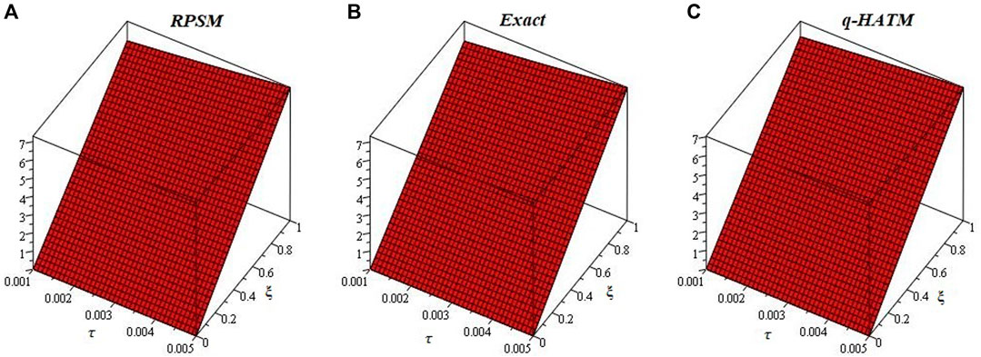
FIGURE 1. 3D plots of (A) RPSM (B) Exact (C) q-HATM-solutions at δ = 1 of Example 4.1.

FIGURE 2

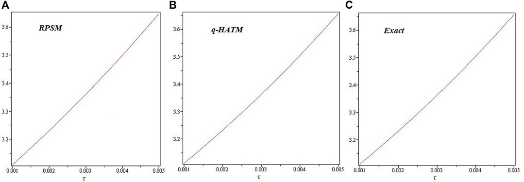
FIGURE 2. 2D plots of (A) RPSM (B) Exact (C) q-HATM-solutions at δ = 1 of Example 4.1.

FIGURE 3

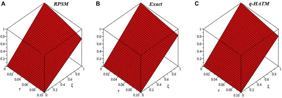
FIGURE 3. 3D plots of (A) RPSM (B) q-HATM-solutions at δ = 1, 0.9 of Example 4.1.

FIGURE 4

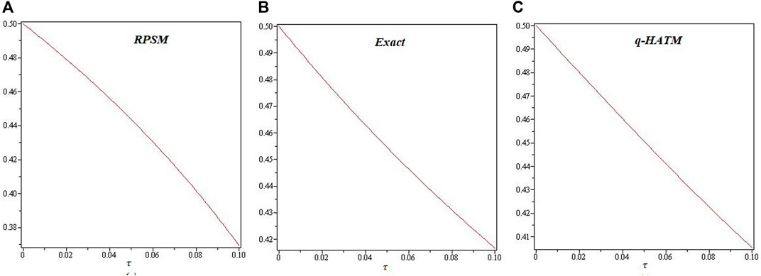
FIGURE 4. 3D plots of (A) RPSM (B) Exact (C) q-HATM-solutions at δ = 1 of Example 4.2.

FIGURE 5

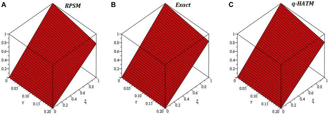
FIGURE 5. 2D plots of (A) RPSM (B) Exact (C) q-HATM-solutions at δ = 1 of Example 4.2.

FIGURE 6

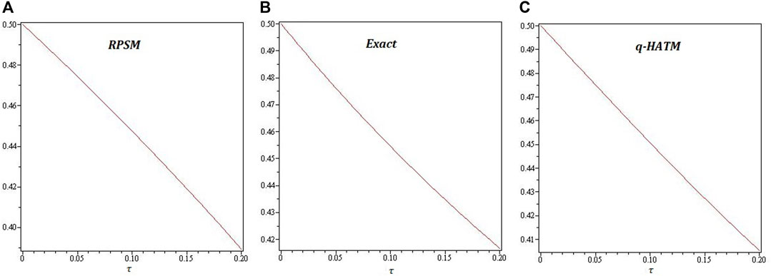
FIGURE 6. The 3D plots of (A) RPSM and (B) q-HATM solutions of example 4.2 at δ = 1 and δ = 0.9.

FIGURE 7

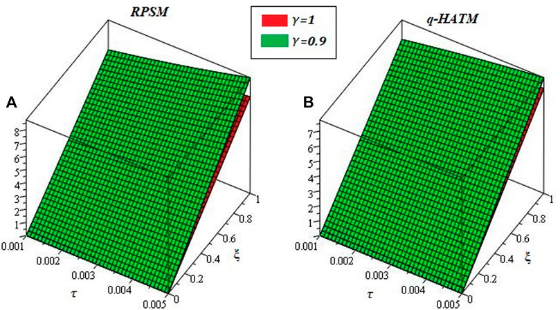
FIGURE 7. 3D plots of (A) RPSM (B) Exact (C) q-HATM-solutions at δ = 1 of Example 4.3.

FIGURE 8

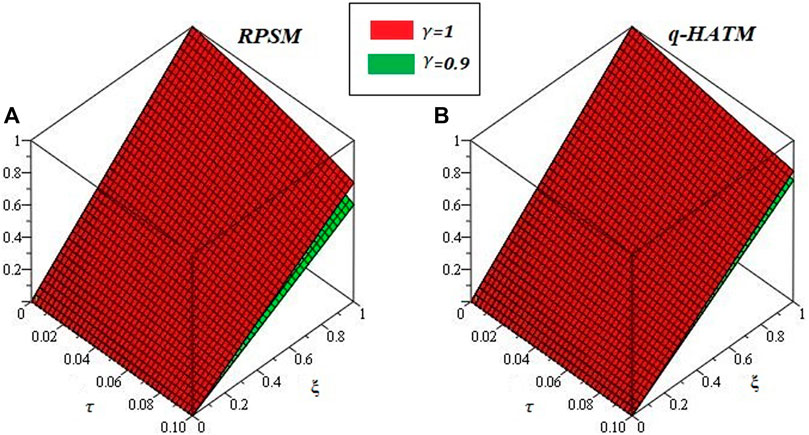
FIGURE 8. 2D plots of (A) RPSM (B) Exact (C) q-HATM-solutions at δ = 1 of Example 4.3.

FIGURE 9

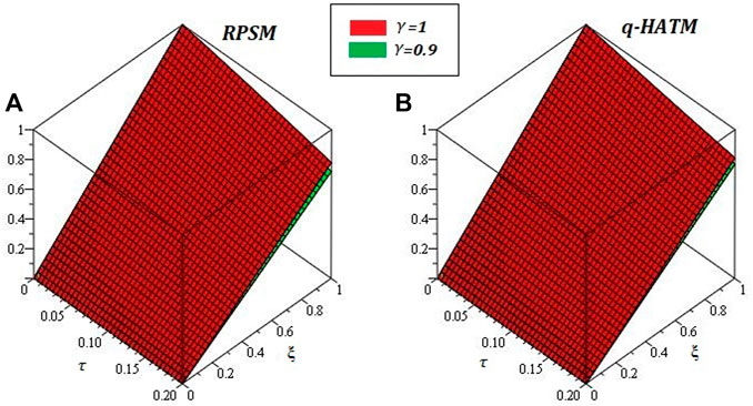
FIGURE 9. 3D plots of (A) RPSM (B) q-HATM-solutions at δ = 1, 0.9 of Example 4.3.

TABLE 1

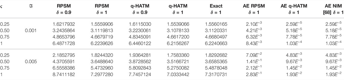
TABLE 1. A comparison of RPSM, q-HATM and exact for various values of ς and $\mathfrak{I}$.

TABLE 2

TABLE 2. A comparison of RPSM, q-HATM and exact for various values of ς and $\mathfrak{I}$.

TABLE 3

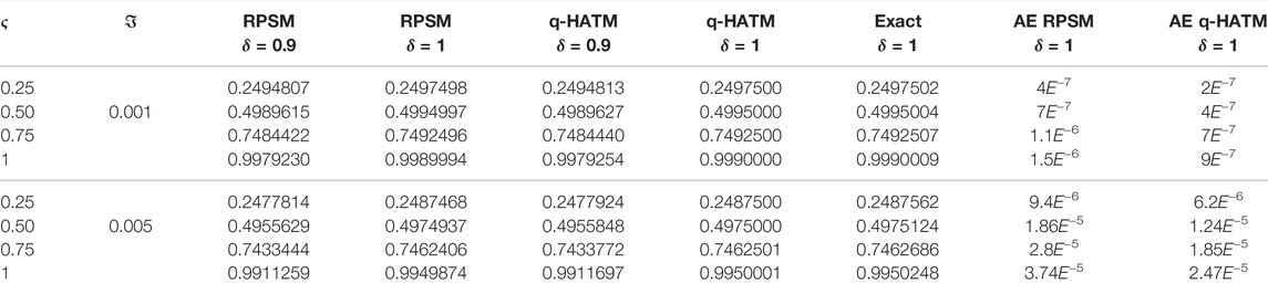
TABLE 3. A comparison of RPSM, q-HATM and exact for various values of ς and $\mathfrak{I}$.

6 Conclusion

In this paper, the solutions of various non-linear fractional KdV equations are presented using two innovative techniques. RPSM and q-HATM are the most simple and straightforward procedures which can be used effectively for the solutions FPDEs and their systems. The obtained solutions, using the proposed techniques are displayed through graphs and tables. The solutions comparison has shown a very close contact between the exact, RPSM and q-HATM solutions of the targeted problems. The fractional-order solutions of higher interest and provide the useful information about the dynamics of the targeted problems. The fractional solutions are found convergent towards the actual solution of the targeted problems. The present work fully supports the actual dynamics of the physical phenomena and can be extended for the solutions of other complex and non-linear FPDEs and their systems.

Data Availability Statement

The original contributions presented in the study are included in the article/supplementary material, further inquiries can be directed to the corresponding author.

Author Contributions

HK (Supervision), QK (Methodology), FT (Project administrator), PK (Funding, Draft Writing), GS (Investigation), IU (Methodology), KS (Funding, Draft Writing), FT (Draft writing, visualization).

Funding

The authors acknowledge the financial support provided by the Center of Excellence in Theoretical and Computational Science (TaCS-CoE), KMUTT. This research project is supported by Thailand Science Research and Innovation (TSRI) Basic Research Fund: Fiscal year 2022 under project number FRB650048/0164. Researchers Supporting Project number (RSP2022R440), King Saud University, Riyadh, Saudi Arabia.

Conflict of Interest

The authors declare that the research was conducted in the absence of any commercial or financial relationships that could be construed as a potential conflict of interest.

Publisher’s Note

All claims expressed in this article are solely those of the authors and do not necessarily represent those of their affiliated organizations, or those of the publisher, the editors and the reviewers. Any product that may be evaluated in this article, or claim that may be made by its manufacturer, is not guaranteed or endorsed by the publisher.

References

1. Longhi S. Fractional Schrödinger Equation in Optics. Opt Lett (2015) 40(6):1117–20. doi:10.1364/ol.40.001117

PubMed Abstract | CrossRef Full Text | Google Scholar

2. Din A, Khan A, Zeb A, Sidi Ammi MR, Tilioua M, Torres DFM. Hybrid Method for Simulation of a Fractional COVID-19 Model with Real Case Application. Axioms (2021) 10(4):290. doi:10.3390/axioms10040290

CrossRef Full Text | Google Scholar

3. Ullah S, Khan MA, Farooq M. A New Fractional Model for the Dynamics of the Hepatitis B Virus Using the Caputo-Fabrizio Derivative. The Eur Phys J Plus (2018) 133(6):1–14. doi:10.1140/epjp/i2018-12072-4

CrossRef Full Text | Google Scholar

4. Altaf Khan M, Ullah S, Farooq M. A New Fractional Model for Tuberculosis with Relapse via Atangana-Baleanu Derivative. Chaos, Solitons & Fractals (2018) 116:227–38. doi:10.1016/j.chaos.2018.09.039

CrossRef Full Text | Google Scholar

5. Mahmood S, Shah R, khan H, Arif M. Laplace Adomian Decomposition Method for Multi Dimensional Time Fractional Model of Navier-Stokes Equation. Symmetry (2019) 1111(22):149149. doi:10.3390/sym11020149

CrossRef Full Text | Google Scholar

6. He JH. Nonlinear Oscillation with Fractional Derivative and its Applications. Int Conf vibrating Eng (1998) 98:288–91.

Google Scholar

7. Fellah ZEA, Fellah M, Roncen R, Ongwen NO, Ogam E, Depollier C. Transient Propagation of Spherical Waves in Porous Material: Application of Fractional Calculus. Symmetry (2022) 14(2):233. doi:10.3390/sym14020233

CrossRef Full Text | Google Scholar

8. He JH. Homotopy Perturbation Technique. Comput Methods Appl Mech Eng (1999) 178(3-4):257–62. doi:10.1016/s0045-7825(99)00018-3

CrossRef Full Text | Google Scholar

9. Wu X, Lai D, Lu H. Generalized Synchronization of the Fractional-Order Chaos in Weighted Complex Dynamical Networks with Nonidentical Nodes. Nonlinear Dyn (2012) 69(1):667–83. doi:10.1007/s11071-011-0295-9

CrossRef Full Text | Google Scholar

10. Birajdar GA. Numerical Solution of Time Fractional Navier-Stokes Equation by Discrete Adomian Decomposition Method. Nonlinear Eng (2014) 3(1):21–6. doi:10.1515/nleng-2012-0004

CrossRef Full Text | Google Scholar

11. Momani S, Odibat Z. Analytical Solution of a Time-Fractional Navier-Stokes Equation by Adomian Decomposition Method. Appl Maths Comput (2006) 177(2):488–94. doi:10.1016/j.amc.2005.11.025

CrossRef Full Text | Google Scholar

12. Tarasov V. On History of Mathematical Economics: Application of Fractional Calculus. Mathematics (2019) 7(6):509. doi:10.3390/math7060509

CrossRef Full Text | Google Scholar

13. Veeresha P, Prakasha DG, Baskonus HM. New Numerical Surfaces to the Mathematical Model of Cancer Chemotherapy Effect in Caputo Fractional Derivatives. Chaos (2019) 29(1):013119. doi:10.1063/1.5074099

PubMed Abstract | CrossRef Full Text | Google Scholar

14. Nasrolahpour H. A Note on Fractional Electrodynamics. Commun Nonlinear Sci Numer Simulation (2013) 18(9):2589–93. doi:10.1016/j.cnsns.2013.01.005

CrossRef Full Text | Google Scholar

15. Yang XJ, Abdel-Aty M, Cattani C. A New General Fractional-Order Derivataive with Rabotnov Fractional-Exponential Kernel Applied to Model the Anomalous Heat Transfer. Therm Sci (2019) 23(3 Part A):1677–81. doi:10.2298/tsci180320239y

CrossRef Full Text | Google Scholar

16. Abdel-Aty A-H, Khater MMA, Attia RAM, Abdel-Aty M, Eleuch H. On the New Explicit Solutions of the Fractional Nonlinear Space-Time Nuclear Model. Fractals (2020) 28(08):2040035. doi:10.1142/s0218348x20400356

CrossRef Full Text | Google Scholar

17. Kang Y, Mao S, Zhang Y. Fractional Time-Varying Grey Traffic Flow Model Based on Viscoelastic Fluid and its Application. Transportation Res B: methodological (2022) 157:149–74. doi:10.1016/j.trb.2022.01.007

CrossRef Full Text | Google Scholar

18. Chaurasia VBL, Kumar D. Solution of the Time-Fractional Navier–Stokes Equation. Gen Math Notes (2011) 4(2):49–59.

Google Scholar

19. Khan MA, Ullah S, Okosun KO, Shah K. A Fractional Order pine Wilt Disease Model with Caputo–Fabrizio Derivative. Adv Difference Equations (2018) 2018(1):1–18. doi:10.1186/s13662-018-1868-4

CrossRef Full Text | Google Scholar

20. Singh J, Kumar D, Baleanu D. On the Analysis of Fractional Diabetes Model with Exponential Law. Adv Difference Equations (2018) 2018(1):1–15. doi:10.1186/s13662-018-1680-1

CrossRef Full Text | Google Scholar

21. Bertsias P, Kapoulea S, Psychalinos C, Elwakil AS. A Collection of Interdisciplinary Applications of Fractional-Order Circuits. In: Fractional Order Systems. Cambridge, MA, USA: Academic Press (2022). p. 35–69. doi:10.1016/b978-0-12-824293-3.00007-7

CrossRef Full Text | Google Scholar

22. Hilfer R. Applications of Fractional Calculus in Physics. Orlando: World Scientific (1999).

Google Scholar

23. Kilbas AA, Srivastava HM, Trujillo JJ. Theory and Applications of Fractional Differential Equations (Vol. 204). Amsterdam, Netherlands: Elsevier (2006).

Google Scholar

24. Das S. A Note on Fractional Diffusion Equations. Chaos, Solitons & Fractals (2009) 42(4):2074–9. doi:10.1016/j.chaos.2009.03.163

CrossRef Full Text | Google Scholar

25. Barbosa R, Tenreiro Machado JA, Ferreira IM. PID Controller Tuning Using Fractional Calculus Concepts. Fractional calculus Appl Anal (2004) 7:121–34.

Google Scholar

26. Machado JA. Analysis and Design of Fractional-Order Digital Control Systems. SAMS (1997) 27:107–22.

Google Scholar

27. Machado JA, Jesus IS, Cunha JB, Tar JK. Fractional Dynamics and Control of Distributed Parameter Systems. Intell Syst Serv Mankind (2004) 2014:295–305.

Google Scholar

28. Kumar D, Singh J, Kumar S. Numerical Computation of Nonlinear Fractional Zakharov-Kuznetsov Equation Arising in Ion-Acoustic Waves. J Egypt Math Soc (2014) 22(3):373–8. doi:10.1016/j.joems.2013.11.004

CrossRef Full Text | Google Scholar

29. Kumar R, Koundal R. Generalized Least Square Homotopy Perturbation for System FPDEs. arXiv preprint arXiv:1805.06650 (2018).

Google Scholar

30. Demir A, Erman S, Özgür B, Korkmaz E. Analysis of Fractional Partial Differential Equations by Taylor Series Expansion. Bound Value Probl (2013) 2013(1):68. doi:10.1186/1687-2770-2013-68

CrossRef Full Text | Google Scholar

31. Baleanu D, Tenerio Machado JA, Cattani c., Baleanu MC, Yang XJ. Local Fractional Variational Iteration and Decomposition Method for Wave Equation on Cantor Sets within Local Fractional Operators. Abstract Appl Anal (2013) 2014:535048. doi:10.1155/2014/535048

CrossRef Full Text | Google Scholar

32. Khan H, Shah R, Kumam P, Baleanu D, Arif M. Laplace Decomposition for Solving Nonlinear System of Fractional Order Partial Differential Equations. Adv Difference Equations (2020) 2020(1):1–18. doi:10.1186/s13662-020-02839-y

CrossRef Full Text | Google Scholar

33. Alderremy AA, Khan H, Shah R, Aly S, Baleanu D. The Analytical Analysis of Time-Fractional Fornberg-Whitham Equations. Mathematics (2020) 8(6):987. doi:10.3390/math8060987

CrossRef Full Text | Google Scholar

34. Shah R, Khan H, Baleanu D, Kumam P, Arif M. A Novel Method for the Analytical Solution of Fractional Zakharov–Kuznetsov Equations. Adv Difference Equations (2019) 2019(1):1–14. doi:10.1186/s13662-019-2441-5

CrossRef Full Text | Google Scholar

35. Srivastava HM, Shah R, Khan H, Arif M. Some Analytical and Numerical Investigation of a Family of Fractional‐order Helmholtz Equations in Two Space Dimensions. Math Meth Appl Sci (2020) 43(1):199–212. doi:10.1002/mma.5846

CrossRef Full Text | Google Scholar

36. Prakash A, Kaur H. Numerical Solution for Fractional Model of Fokker-Planck Equation by Using Q-HATM. Chaos, Solitons & Fractals (2017) 105:99–110. doi:10.1016/j.chaos.2017.10.003

CrossRef Full Text | Google Scholar

37. Singh J, Kumar D, Swroop R. Numerical Solution of Time- and Space-Fractional Coupled Burgers' Equations via Homotopy Algorithm. Alexandria Eng J (2016) 55:1753–63. doi:10.1016/j.aej.2016.03.028

CrossRef Full Text | Google Scholar

38. Jafari H, Nazari M, Baleanu D, Khalique CM. A New Approach for Solving a System of Fractional Partial Differential Equations. Comput Maths Appl (2013) 66(5):838–43. doi:10.1016/j.camwa.2012.11.014

CrossRef Full Text | Google Scholar

39. Mustahsan M, Younas HM, Iqbal S, Rathore S, Nisar KS, Singh J. An Efficient Analytical Technique for Time-Fractional Parabolic Partial Differential Equations. Front Phys (2020) 8:131. doi:10.3389/fphy.2020.00131

CrossRef Full Text | Google Scholar

40. Wang Q. Numerical Solutions for Fractional KdV-Burgers Equation by Adomian Decomposition Method. Appl Maths Comput (2006) 182(2):1048–55. doi:10.1016/j.amc.2006.05.004

CrossRef Full Text | Google Scholar

41. Daftardar-Gejji V, Bhalekar S. Solving Multi-Term Linear and Non-linear Diffusion-Wave Equations of Fractional Order by Adomian Decomposition Method. Appl Maths Comput (2008) 202(1):113–20. doi:10.1016/j.amc.2008.01.027

CrossRef Full Text | Google Scholar

42. Ismail GM, Abdl-Rahim HR, Abdel-Aty A, Kharabsheh R, Alharbi W, Abdel-Aty M. An Analytical Solution for Fractional Oscillator in a Resisting Medium. Chaos, Solitons & Fractals (2020) 130:109395. doi:10.1016/j.chaos.2019.109395

CrossRef Full Text | Google Scholar

43. Chamekh M, Elzaki TM. Explicit Solution for Some Generalized Fluids in Laminar Flow with Slip Boundary Conditions. J Math Comput Sci. (2018) 18:272–81. doi:10.22436/jmcs.018.03.03

CrossRef Full Text | Google Scholar

44. Liu H, Khan H, Shah R, Alderremy AA, Aly S, Baleanu D. On the Fractional View Analysis of Keller–Segel Equations with Sensitivity Functions. Complexity (2020) 2020:2371019. doi:10.1155/2020/2371019

CrossRef Full Text | Google Scholar

45. Abdulaziz O, Hashim I, Ismail ES. Approximate Analytical Solution to Fractional Modified KdV Equations. Math Comput Model (2009) 49(1-2):136–45. doi:10.1016/j.mcm.2008.01.005

CrossRef Full Text | Google Scholar

46. Srivastava HM, Saad KM, Hamanah WM. Certain New Models of the Multi-Space Fractal-Fractional Kuramoto-Sivashinsky and Korteweg-De Vries Equations. Mathematics (2022) 10(7):1089. doi:10.3390/math10071089

CrossRef Full Text | Google Scholar

47. Wang Q. Homotopy Perturbation Method for Fractional KdV Equation. Appl Maths Comput (2007) 190(2):1795–802. doi:10.1016/j.amc.2007.02.065

CrossRef Full Text | Google Scholar

48. Ali KK, Dutta H, Yilmazer R, Noeiaghdam S. On the New Wave Behaviors of the Gilson-Pickering Equation. Front Phys (2020) 8:54. doi:10.3389/fphy.2020.00054

CrossRef Full Text | Google Scholar

49. Korpinar Z, Tchier F, Inc M. On Optical Solitons of the Fractional (3+1)-Dimensional NLSE with Conformable Derivatives. Front Phys (2020) 8:87. doi:10.3389/fphy.2020.00087

CrossRef Full Text | Google Scholar

50. Uddin MF, Hafez MG, Hwang I, Park C. Effect of Space Fractional Parameter on Nonlinear Ion Acoustic Shock Wave Excitation in an Unmagnetized Relativistic Plasma. Front Phys (2022) 2022:766. doi:10.3389/fphy.2021.766035

CrossRef Full Text | Google Scholar

51. Rehman Mu., Khan RA. Numerical Solutions to Initial and Boundary Value Problems for Linear Fractional Partial Differential Equations. Appl Math Model (2013) 37(7):5233–44. doi:10.1016/j.apm.2012.10.045

CrossRef Full Text | Google Scholar

52. Akinlar MA, Secer A, Bayram M. Numerical Solution of Fractional Benney Equation. Appl Math Inf Sci (2014) 8(4):1633–7. doi:10.12785/amis/080418

CrossRef Full Text | Google Scholar

53. Secer A, Akinlar MA, Cevikel A. Similarity Solutions for Multiterm Time-Fractional Diffusion Equation. Adv Differ Equ (2012) 2012:7304659. doi:10.1155/2016/7304659

CrossRef Full Text | Google Scholar

54. Kurulay M, Bayram M. Approximate Analytical Solution for the Fractional Modified KdV by Differential Transform Method. Commun nonlinear Sci Numer simulation (2010) 15(7):1777–82. doi:10.1016/j.cnsns.2009.07.014

CrossRef Full Text | Google Scholar

55. Kurulay M, Akinlar MA, Ibragimov R. Computational Solution of a Fractional Integro-Differential Equation. Abstract Appl Anal (2013) 2013:865952. doi:10.1155/2013/865952

CrossRef Full Text | Google Scholar

56. Srivastava HM, Saad KM. Some New and Modified Fractional Analysis of the Time-Fractional Drinfeld-Sokolov-Wilson System. Chaos (2020) 30(11):113104. doi:10.1063/5.0009646

PubMed Abstract | CrossRef Full Text | Google Scholar

57. Khader MM, Saad KM. Numerical Studies of the Fractional Korteweg-De Vries, Korteweg-De Vries-Burgers' and Burgers' Equations. Proc Natl Acad Sci India, Sect A Phys Sci (2021) 91(1):67–77. doi:10.1007/s40010-020-00656-2

CrossRef Full Text | Google Scholar

58. Shah R, Khan H, Baleanu D, Kumam P, Arif M. A Semi-analytical Method to Solve Family of Kuramoto-Sivashinsky Equations. J Taibah Univ Sci (2020) 14(1):402–11. doi:10.1080/16583655.2020.1741920

CrossRef Full Text | Google Scholar

59. Abu O. Arqub, Series Solution of Fuzzy Differential Equation under Strongly Generalized Differentiability. J Adv Res Appl Maths (2013) 5:31. doi:10.5373/jaram.1447.051912

CrossRef Full Text | Google Scholar

60. Caputo M. Elasticita e Dissipazione. Bologna: Zanichelli (1969).

Google Scholar

61. Caputo M. Linear Models of Dissipation Whose Q Is Almost Frequency Independent--II. Geophys J Int (1967) 13:529–39. doi:10.1111/j.1365-246x.1967.tb02303.x

CrossRef Full Text | Google Scholar

62. Miller KS, Ross B. An Introduction to the Fractional Calculus and Fractional Differential Equation. New York: Wiley (1993).

Google Scholar

63. Tchier F, Inc M, Korpinar ZS, Baleanu D. Solution of the Time Fractional Reaction-Diffusion Equations with Residual Power Series Method. Adv Mech Eng (2016) 8:1–10. doi:10.1177/1687814016670867

CrossRef Full Text | Google Scholar

64. Prakasha DG, Veeresha P, Baskonus HM. Residual Power Series Method for Fractional Swift-Hohenberg Equation. Fractal Fract (2019) 3(1):9. doi:10.3390/fractalfract3010009

CrossRef Full Text | Google Scholar

65. Abu Arqub O. Series Solution of Fuzzy Differential Equations under Strongly Generalized Differentiability. J Adv Res Appl Maths (2013) 5(1):31–52. doi:10.5373/jaram.1447.051912

CrossRef Full Text | Google Scholar

66. Abu Arqub O, El-Ajou A, Bataineh AS, Hashim I. A Representation of the Exact Solution of Generalized Lane-Emden Equations Using a New Analytical Method. Abstract Appl Anal (2013) 2013:378593. doi:10.1155/2013/378593

CrossRef Full Text | Google Scholar

67. Prakash A, Kaur H. Q-Homotopy Analysis Transform Method for Space and Time-Fractional KdV-Burgers Equation. Nonlinear Sci Lett A (2018) 9(1):44–61.

Google Scholar

68. Sontakke B, Shaikh A. The New Iterative Method for Approximate Solutions of Time Fractional Kdv, K(2,2), Burgers, and Cubic Boussinesq Equations. Arjom (2016) 1:1–10. doi:10.9734/arjom/2016/29279

CrossRef Full Text | Google Scholar