New concepts on level graphs of vague graphs with application in medicine

Shi, Xiaolong; Jiang, Wubian; Khan, Aysha; Akhoundi, Maryam

doi:10.3389/fphy.2023.1130765

ORIGINAL RESEARCH article

Front. Phys., 21 February 2023

Sec. Statistical and Computational Physics

Volume 11 - 2023 | https://doi.org/10.3389/fphy.2023.1130765

New concepts on level graphs of vague graphs with application in medicine

Xiaolong Shi¹

Wubian Jiang²*

Aysha Khan³

Maryam Akhoundi⁴

¹Institute of Computing Science and Technology, Guangzhou University, Guangzhou, China
²Renmin Hospital of Wuhan University Outpatient Management Service Department, Wuhan, China
³Department of Mathematics, Prince Sattam Bin Abdulaziz University, Al-Kharj, Saudi Arabia
⁴Clinical Research Development Unit of Rouhani Hospital, Babol University of Medical Sciences, Babol, Iran

Vague graphs (VGs), belonging to the fuzzy graph (FG) family, have good capabilities when facing problems that cannot be expressed by FGs. When an element membership is unclear, neutrality is a good option that can be well-supported by a VG. The previous definitions limitations in FG have led us to offer new definitions in VGs. Therefore, this study introduces the notion of vague edge graph (VEG) $\hat{ζ} = (V, N)$ , in which V is a crisp vertex set and N is a vague relation (VR) on M, presenting some of its properties. Using λ-level graphs (LGs) and (λ, δ)-LGs, we characterize VG ζ = (M, N), where M is a vague set (VS) on V and N is a VR on V. Medical diagnosis is one of the most sensitive and important issues in the medical sciences. If it is not done properly, the patient will suffer irreparable damage. Therefore, an application of VG in the diagnosis of the disease is expressed.

1 Introduction

After the introduction of fuzzy sets (FSs) [1], the fuzzy set theory is included as a large research field. Since then, the theory of FSs has become a vigorous area of research in different disciplines, including life sciences, management science, statistic, graph theory, and automata theory. Graphs from ancient times to the present day have played a very important role in various fields, including computer science and social networks, so that, with the help of the nodes and edges of a graph, the relationships between objects and elements in a social group can be easily introduced.

A fuzzy graph (FG) is one of the most widely used topics in fuzzy theory, which has been studied by many researchers. One of the advantages of FG is its flexibility in reducing time and costs in economic issues, which has been welcomed by all managers of institutions and companies. Gau and Buehrer [2] organized the FS theory by presenting the VS notion by changing the value of an element in a set with a subinterval of [0,1]. A VS is more initiative and helpful due to the existence of false membership degrees. Kauffman [3] introduced FGs using Zadeh’s fuzzy relation (FR) [4, 5]. However, Rosenfeld [6] presented another detailed definition, such as paths, cycles, and connectedness. Mordeson and Chang-Shyh [7] defined operations on FGs. References [8, 9] introduced certain types of product bipolar FGs and some operations and densities of m-polar FGs. Das et al. [10] presented generalized neutrosophic competition graphs. Bhattacharya [11] identified some remarks on FGs. Mordeson and Nair [12] studied several concepts of FGs. Mahapatra [13] introduced radio FGs and frequency assignment in radio stations. References [14–16] investigated new definitions of vague graphs, and references [17–20] defined several concepts on VGs and neutrosophic competition graphs. Shoaib et al. [21] studied complex Pythagorean FGs.

VG is a type of FG. VGs have a variety of applications in other sciences, including biology, psychology, management, and medicine. They are used to find the most effective person in an organization or institution. Likewise, a VG can focus on determining the uncertainty combined with the inconsistent and indeterminate information of any real-world problem in which FGs may not lead to adequate results. The nodes in this graph represent the individuals, and the edges show the extent of the relationship between employees. Furthermore, VGs play a very important role in the field of medical sciences and are used to diagnose diseases and reduce the costs of hospitals and medical clinics using the concept of domination and covering. Ramakrishna [22] recommended the VG notion and evaluated some of its features. Borzooei and Rashmanlou [23, 24] introduced new concepts in VGs. Sunitha and Vijayakumar [25] presented a complement of FGs. Kosari et al. and Kou et al. [26, 27] studied new results in VG structures. References [28–30] defined dominating and equitable dominating sets in VGs. Shi and Kosari [31] investigated the global dominating set in product-VGs. Shao et al. [32] introduced a bondage set and bondage number in intuitionistic FG. VG is used to illustrate real-world phenomena using vague models in a variety of fields, including technology, social networking, and biological networks. Therefore, in this study, we presented the notion of VEG and introduced some of its properties. Likewise, we characterized VG ζ = (M, N), where M is a VS and N is a VR. Some operations, including CP, LP, SP, and cross-product on VGs, have been defined. Finally, an application of VG in medical diagnosis has been given.

2 Preliminaries

In this section, we introduce some basic concepts of VGs.

A graph is an ordered pair ζ* = (V, E), where V is the set of nodes of ζ* and $E \in \tilde{V^{2}}$ is the set of edges of ζ*. Two nodes p and q in a graph $G^{*}$ are said to be neighbors in $G^{*}$ , if {p, q} is in an edge of $G^{*}$ .

Definition 2.1. A fuzzy graph (FG) is a pair ς = (τ, ν) with a set X [12]; then τ is a fuzzy set (FS) in X, and ν is a fuzzy relation (FR) in X × X, so that

$γ (p q) \leq \min {τ (p), τ (q)},$

for all pq ∈ X × X.

Definition 2.2. A VS is a pair (t_M, f_M) on set X [2], where t_M and f_M are real-valued functions, which can be presented on V → [0, 1] so that t_M(p) + f_M(p) ≤ 1 and ∀p ∈ X.

Definition 2.3. A VG is defined as a pair ζ = (M, N) [22],where M = (t_M, f_M) is a VS on V and N = (t_N, f_N) is a VS on E ⊆ V × V so that for each pq ∈ E, t_N (pq) ≤ t_M(p) ∧ t_M(q) and f_N (pq) ≥ f_N(p) ∨ f_N(q).

Definition 2.4. A VEG on a non-empty set V is an ordered pair of the form $\hat{ζ} = (V, N)$ , where V is a crisp vertex set (CVS) and N is a VR on V so that t_N (pq) ≤ min{t_M(p), t_M(q)}, f_N (pq) ≥ max{f_M(p), f_M(q)}, and 0 ≤ t_N (pq) + f_N (pq) ≤ 1, for all pq ∈ E.

We consider VEGs with CVS, that is, VGs $\hat{ζ} = (V, N)$ , that is, t_M(p) = 1, f_M(p) = 0, ∀p ∈ V, and edges with true membership and false membership degrees in [0,1].

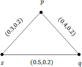
Example 2.5. Consider a simple graph (SG) ζ* = (V, E) [24]so that V = {p, q, s} and E = {pq, qs, ps}. Let N be a VR on V described by N = {(pq, 0.4, 0.2), (qs, 0.5, 0.2), (ps, 0.3, 0.2)}. Clearly, $\hat{ζ} = (V, N)$ is a VEG with CVS and VS of edges (see Figure 1).

FIGURE 1

FIGURE 1. Vague edge graph $\hat{ζ} = (V, N)$ .

3 Vague graphs by level graphs

Definition 3.1. Suppose that M = (t_m, f_M) is a VS on V. Then, the set M_(λ,δ) = {p ∈ V|t_M(p) ≥ λ, f_M(p) ≤ δ}, where (λ, δ) ∈ [0, 1] × [0, 1] and λ + δ ≤ 1 is named the (λ, δ)-level set of M. Let N = (t_N, f_N) be a VR on V. Then, the set N_(λ,δ) = {pq ∈ V × V|t_N (pq) ≥ λ, f_M(pq) ≤ δ}, where (λ, δ) ∈ [0, 1] × [0, 1] and λ + δ ≤ 1 is called (λ, δ)-LG. In the case of λ = δ, where λ ≤ 1, we write LG by ζ_α instead of ζ_(λ,δ). Note that

$\begin{matrix} M_{(λ, δ)} = {p \in V | t_{M} (p) \geq λ} \cap {p \in V | f_{M} (p) \leq δ} = U (t; λ) \cap L (f; δ), \\ N_{(λ, δ)} = {p q \in V \times V | t_{N} (p q) \geq λ} \cap {p q \in V \times V | f_{N} (p q) \leq δ} = U (t; λ) \cap L (f; δ) . \end{matrix}$

Remark 3.2. The level graph ζ_(λ,δ) = (M_(λ,δ), N_(λ,δ)) is a subgraph of ζ* = (V, E).

Example 3.3. Consider an SG ζ* = (V, E) so that V = {p, q, r, s} and E = {pq, qr, rs, ps, pr, qs}. From Figure 2, we get that ζ = (M, N) is a VG.Take λ = 0.5. We have M_0.5 = {s, r} and N_0.5 = {rs}. Obviously, the 0.5-LG ζ_0.5 is a subgraph of ζ*.Now, we take λ = 0.2 and δ = 0.3. By Definition 3.1, we have M_(0.2,0.3) = {p, r, s} and N_(0.2,0.3) = {ps}. Clearly, (0.2,0.3)-LG ζ_(0.2,0.3) is a subgraph of ζ*.

FIGURE 2

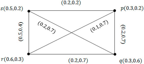
FIGURE 2. Vague graph ζ.

Theorem 3.4. ζ = (M, N) is a VG if ζ_(λ,δ) is a crisp graph for each pair (λ, δ) ∈ [0, 1] × [0, 1] and λ + δ ≤ 1.Proof. Suppose ζ is a VG. For each (λ, δ) ∈ [0, 1] × [0, 1], we take pq ∈ N_(λ,δ). Then, t_N (pq) ≥ λ and f_N (pq) ≤ δ. Since ζ is a VG, it follows that

$\begin{matrix} λ \leq t_{N} (p q) \leq \min (t_{M} (p), t_{M} (q)), \\ δ \geq f_{N} (p q) \geq \max (f_{M} (p), f_{M} (q)) . \end{matrix}$

It shows that λ ≤ t_M(p), λ ≤ t_M(q), δ ≥ f_M(p), and δ ≥ f_M(q); that is, p, q ∈ M_(λ,δ). Hence, ζ_(λ,δ) is a graph for each (λ, δ) ∈ [0, 1] × [0, 1]. Conversely, suppose ζ_(λ,δ) is a graph for all (λ, δ) ∈ [0, 1] × [0, 1]. For each $p q \in \tilde{V^{2}}$ , let f_N (pq) = δ and t_N (pq) = λ. Then, pq ∈ N_(λ,δ). Since ζ_(λ,δ) is a graph, we have p, q ∈ M_(λ,δ), so t_M(p) ≥ λ, t_M(q) ≥ λ, f_M(p) ≤ δ, and f_M(q) ≤ δ. Therefore,

$\begin{matrix} t_{N} (p q) = λ \leq \min (t_{M} (p), t_{M} (q)), \\ f_{N} (p q) = δ \geq \max (f_{M} (p), f_{M} (q)), \end{matrix}$

that is, ζ = (M, N) is a VG. Definition 3.5. Suppose ζ₁ = (M₁, N₁) and ζ₂ = (M₂, N₂) are two VGs of $ζ_{1}^{*} = (V_{1}, E_{1})$ and $ζ_{2}^{*} = (V_{2}, E_{2})$ , respectively. The Cartesian product (CP) ζ₁ × ζ₂ is the pair (M, N) of VSs defined on the CP $ζ_{1}^{*} \times ζ_{2}^{*}$ so that

$\begin{matrix} (i) \{\begin{cases} t_{M} (p_{1}, p_{2}) = \min (t_{M_{1}} (p_{1}), t_{M_{2}} (p_{2})) \\ f_{M} (p_{1}, p_{2}) = \max (f_{M_{1}} (p_{1}), f_{M_{2}} (p_{2})), \forall (p_{1}, p_{2}) \in V_{1} \times V_{2}, \end{cases} \\ (i i) \{\begin{cases} t_{N} ((p, p_{2}) (p, q_{2})) = \min (t_{M_{1}} (p), t_{N_{2}} (p_{2} q_{2})) \\ f_{M} ((p, p_{2}) (p, q_{2})) = \max (f_{M_{1}} (p), f_{N_{2}} (p_{2} q_{2})), \forall p \in V_{1} a n d p_{2} q_{2} \in E_{2}, \end{cases} \\ (i i i) \{\begin{cases} t_{N} ((p_{1}, r) (q_{1}, r)) = \min (t_{N_{1}} (p_{1} q_{1}), t_{M_{2}} (r)) \\ f_{M} ((p_{1}, r) (q_{1}, r)) = \max (f_{N_{1}} (p_{1} q_{1}), f_{M_{2}} (r)), \forall r \in V_{2} a n d p_{1} q_{1} \in E_{1} . \end{cases} \end{matrix}$

Theorem 3.6. ζ = (M, N) is the CP of ζ₁ and ζ₂ if and only if each pair (λ, δ) ∈ [0, 1] × [0, 1] and λ + δ ≤ 1, (λ, δ)-LG ζ_(λ,δ) is the CP of ${(ζ_{1})}_{(λ, δ)}$ and ${(ζ_{2})}_{(λ, δ)}$ .Proof. Assume ζ = (M, N) is the CP of ζ₁ and ζ₂. For each (λ, δ) ∈ [0, 1] × [0, 1], if (p, q) ∈ M_(λ,δ), then

$\min (t_{M_{1}} (p), t_{M_{2}} (q)) = t_{M} (p, q) \geq δ$

and

$\max (f_{M_{1}} (p), f_{M_{2}} (q)) = f_{M} (p, q) \leq λ .$

Hence, $p \in {(M_{1})}_{(λ, δ)}$ and $q \in {(M_{2})}_{(λ, δ)}$ ; that is $(p, q) \in {(M_{1})}_{(λ, δ)} \times {(M_{2})}_{(λ, δ)}$ . Therefore, $M_{(λ, δ)} \subseteq {(M_{1})}_{(λ, δ)} \times {(M_{2})}_{(λ, δ)}$ .Now if $(p, q) \in {(M_{1})}_{(λ, δ)} \times {(M_{2})}_{(λ, δ)}$ , then $p \in {(M_{1})}_{(λ, δ)}$ and $q \in {(M_{2})}_{(λ, δ)}$ . It follows $\min (t_{M_{1}} (p), t_{M_{2}} (q)) \geq δ$ and $\max (f_{M_{1}} (p), f_{M_{2}} (q)) \leq λ$ . Since (M, N) is the CP of ζ₁ and ζ₂, t_M(p, q) ≥ δ and f_M(p, q) ≤ λ; that is, (p, q) ∈ M_(λ,δ). So, ${(M_{1})}_{(λ, δ)} \times {(M_{2})}_{(λ, δ)} \subseteq M_{(λ, δ)}$ . Thus, ${(M_{1})}_{(λ, δ)} \times {(M_{2})}_{(λ, δ)} = M_{(λ, δ)}$ . Now, we prove N_(λ,δ) = E, where E is the edge set of the CP of ${(ζ_{1})}_{(λ, δ)} \times {(ζ_{2})}_{(λ, δ)}$ and ∀(λ, δ) ∈ [0, 1] × [0, 1]. Suppose (p₁, p₂) (q₁, q₂) ∈ N_(λ,δ). Then, $t_{N} ((p_{1}, p_{2}) (q_{1}, q_{2})) \geq δ$ and $t_{N} ((p_{1}, p_{2}) (q_{1}, q_{2})) \leq λ$ . Since (M, N) is the CP of ζ₁ and ζ₂, one of the following cases holds:(i) p₁ = q₁ and p₂q₂ ∈ E₂.(ii) p₂ = q₂ and p₁q₁ ∈ E₁.For case (i), we have

$\begin{matrix} t_{N} ((p_{1}, p_{2}) (q_{1}, q_{2})) = \min (t_{M_{1}} (p_{1}), t_{M_{2}} (p_{2} q_{2})) \geq δ, \\ f_{N} ((p_{1}, p_{2}) (q_{1}, q_{2})) = \max (f_{M_{1}} (p_{1}), f_{N_{2}} (p_{2} q_{2})) \leq λ . \end{matrix}$

So, $t_{M_{1}} (p_{1}) \geq δ$ , $f_{M_{1}} (p_{1}) \leq λ$ , $t_{N_{2}} (p_{2} q_{2}) \geq δ$ , and $f_{N_{2}} (p_{2} q_{2}) \leq λ$ . It follows that $p_{1} = q_{1} \in {(M_{1})}_{(λ, δ)}$ and $p_{2} q_{2} \in {(N_{2})}_{(λ, δ)}$ ; that is, (p₁, p₂) (q₁, q₂) ∈ E.Similarly, for case (ii), we get (p₁, p₂) (q₁, q₂) ∈ E. Thus, N_(λ,δ) ⊆ E. For each (p, p₂) (p, q₂) ∈ E, $t_{M_{1}} (p) \geq δ$ , $f_{M_{1}} (p) \leq λ$ , $t_{N_{2}} (p_{2} q_{2}) \geq δ$ , and $f_{N_{2}} (p_{2} q_{2}) \leq λ$ . Since (M, N) is the CP of ζ₁ and ζ₂, we have

$\begin{matrix} t_{N} ((p, p_{2}) (p, q_{2})) = \min (t_{M_{1}} (p), t_{N_{2}} (p_{2} q_{2})) \geq δ, \\ f_{M} ((p, p_{2}) (p, q_{2})) = \max (f_{M_{1}} (p), f_{N_{2}} (p_{2} q_{2})) \leq λ . \end{matrix}$

Therefore, (p, p₂) (p, q₂) ∈ N_(λ,δ).In the same way, for each (p₁, r) (q₁, r) ∈ E, we get (p₁, r) (q₁, r) ∈ N_(λ,δ). So, E ⊆ N_(λ,δ) and N_(λ,δ) = E.The converse part is obvious.Definition 3.7. Let ζ₁ and ζ₂ be two VGs of $ζ_{1}^{*} = (V_{1}, E_{1})$ and $ζ_{2}^{*} = (V_{2}, E_{2})$ , respectively. The composition (Co) ζ₁ [ζ₂] is the pair (M, N) of VSs defined on the Co $ζ_{1}^{*} [ζ_{2}^{*}]$ so that

$\begin{matrix} (i) \{\begin{cases} t_{M} (p_{1}, p_{2}) = \min (t_{M_{1}} (p_{1}), t_{M_{2}} (p_{2})), \\ f_{M} (p_{1}, p_{2}) = \max (f_{M_{1}} (p_{1}), f_{M_{2}} (p_{2})), \forall (p_{1}, p_{2}) \in V_{1} \times V_{2} . \end{cases} \\ (i i) \{\begin{cases} t_{N} ((p, p_{2}) (p, q_{2})) = \min (t_{M_{1}} (p), t_{N_{2}} (p_{2} q_{2})), \\ f_{N} ((p, p_{2}) (p, q_{2})) = \max (f_{M_{1}} (p), f_{N_{2}} (p_{2} q_{2})), \forall p \in V_{1} a n d \forall p_{2} q_{2} \in E_{2} . \end{cases} \\ (i i i) \{\begin{cases} t_{N} ((p_{1}, r) (q_{1}, r)) = \min (t_{N_{1}} (p_{1} q_{1}), t_{M_{2}} (r)), \\ f_{N} ((p_{1}, r) (q_{1}, r)) = \max (f_{N_{1}} (p_{1} q_{1}), f_{M_{2}} (r)), \forall r \in V_{2} a n d \forall p_{1} q_{1} \in E_{1} . \end{cases} \\ (i v) \{\begin{cases} t_{N} ((p_{1}, p_{2}) (q_{1}, q_{2})) = \min (t_{M_{2}} (p_{2}), t_{M_{2}} (q_{2}), t_{N_{1}} (p_{1} q_{1})), \\ f_{N} ((p_{1}, p_{2}) (q_{1}, q_{2})) = \max (f_{M_{2}} (p_{2}), f_{M_{2}} (q_{2}), f_{N_{1}} (p_{1} q_{1})), \forall p_{2}, q_{2} \in V_{2} a n d \forall p_{1} q_{1} \in E_{1} t h a t p_{2} \neq q_{2} . \end{cases} \end{matrix}$

Theorem 3.8. ζ = (M, N) is the Co of VGs ζ₁ and ζ₂ if, for every (λ, δ) ∈ [0, 1] × [0, 1] and λ + δ ≤ 1, (λ, δ)-LG ζ_(λ,δ) is the Co of ${(ζ_{1})}_{(λ, δ)}$ and ${(ζ_{2})}_{(λ, δ)}$ .Proof. Let ζ = (M, N) be the Co of ζ₁ and ζ₂. By the definition of ζ₁ [ζ₂] and the same argument as in the proof of Theorem 3.6, we have $M_{(λ, δ)} = {(M_{1})}_{(λ, δ)} \times {(M_{2})}_{(λ, δ)}$ . Now, we prove N_(λ,δ) = E, where E is the edge set of the co ${(ζ_{1})}_{(λ, δ)} [{(ζ_{2})}_{(λ, δ)}]$ , for all (λ, δ) ∈ [0, 1] × [0, 1]. Assume (p₁, p₂) (q₁, q₂) ∈ N_(λ,δ). Then, t_N ((p₁, p₂) (q₁, q₂)) ≥ δ and f_N ((p₁, p₂) (q₁, q₂)) ≤ λ. Since ζ = (M, N) is the Co ζ[ζ₂], one of the following conditions hold:(i) p₁ = q₁ and p₂q₂ ∈ E₂.(ii) p₂ = q₂ and p₁q₁ ∈ E₁.(iii) p₂ ≠ q₂ and p₁q₁ ∈ E₁.For cases (i) and (ii), the same as cases (i) and (ii) in the proof of Theorem 3.6, we get (p₁, p₂) (q₁, q₂) ∈ E. For case (iii), we have

$\begin{matrix} t_{N} ((p_{1}, p_{2}) (q_{1}, q_{2})) = \min (t_{M_{2}} (p_{2}), t_{M_{2}} (q_{2}), t_{N_{1}} (p_{1} q_{1})) \geq δ, \\ f_{N} ((p_{1}, p_{2}) (q_{1}, q_{2})) = \max (f_{M_{2}} (p_{2}), f_{M_{2}} (q_{2}), f_{N_{1}} (p_{1} q_{1})) \leq λ . \end{matrix}$

So, $t_{M_{2}} (p_{2}) \geq δ$ , $t_{M_{2}} (q_{2}) \geq δ$ , $t_{N_{1}} (p_{1} q_{1}) \geq δ$ , $f_{M_{2}} (p_{2}) \leq λ$ , $f_{M_{2}} (q_{2}) \leq λ$ , and $f_{N_{1}} (p_{1} q_{1}) \leq λ$ . It follows that $p_{2} q_{2} \in {(M_{2})}_{(λ, δ)}$ and $p_{1} q_{1} \in {(N_{1})}_{(λ, δ)}$ ; that is, (p₁, p₂) (q₁, q₂) ∈ E. Thus, N_(λ,δ) ⊆ E. For each (p₁, p₂) (q₁, q₂) ∈ E, $t_{M_{1}} (p) \geq δ$ , $f_{M_{1}} (p) \leq λ$ , $t_{N_{2}} (p_{2} q_{2}) \geq δ$ , and $f_{N_{2}} (p_{2} q_{2}) \leq λ$ . Since ζ = (M, N) is the Co of ζ₁ [ζ₂], we get

So, (p, p₂) (p, q₂) ∈ N_(λ,δ). Similarly, for each (p₁, r) (q₁, r) ∈ E, we get (p, p₂) (p, q₂) ∈ N_(λ,δ). For each (p₁, p₂) (q₁, q₂) ∈ E, where p₂ ≠ q₂ and p₁ ≠ q₁, $t_{N_{1}} (p_{1} q_{1}) \geq δ$ , $f_{N_{1}} (p_{1} q_{1}) \leq λ$ , $t_{M_{2}} (q_{2}) \geq δ$ , $f_{M_{2}} (q_{2}) \leq λ$ , $t_{M_{2}} (p_{2}) \geq δ$ , and $f_{M_{2}} (p_{2}) \geq λ$ . Since ζ = (M, N) is the Co of $G_{1} [G_{2}]$ , we have

and then (p₁, p₂) (q₁, q₂) ∈ N_(λ,δ). Hence, E ⊆ N_(λ,δ). Thus, E = N_(λ,δ).Conversely, suppose (M_(λ,δ), N_(λ,δ)), where (λ, δ) ∈ [0, 1] × [0, 1], is the Co of ${(ζ_{1})}_{(λ, δ)}$ and $({(M_{2})}_{(λ, δ)}, {(N_{2})}_{(λ, δ)})$ . In the same way, by the same arguments as in the proof of Theorem 3.6, we get

$\begin{matrix} t_{N} ((p_{1}, p_{2}) (q_{1}, q_{2})) = \min (t_{M_{2}} (p_{2}), t_{M_{2}} (q_{2}), t_{N_{1}} (p_{1} q_{1})), \\ f_{N} ((p_{1}, p_{2}) (q_{1}, q_{2})) = \max (f_{M_{2}} (p_{2}), f_{M_{2}} (q_{2}), f_{N_{1}} (p_{1} q_{1})), \end{matrix}$

∀p₂, q₂ ∈ V₂ (p₂ ≠ q₂) and ∀ p₁q₁ ∈ E₁.This completes the proof.Definition 3.9. Let ζ₁ = (M₁, N₁) and ζ₂ = (M₂, N₂) be two VGs. The union ζ₁ ∪ ζ₂ is defined as the pair (M, N) of VSs described on the union of graphs $ζ_{1}^{*}$ and $ζ_{2}^{*}$ so that

$\begin{matrix} (i) t_{M} (p) = \{\begin{cases} t_{M_{1}} (p) & i f p \in V_{1}, p \notin V_{2}, \\ t_{M_{2}} (p) & i f p \in V_{2}, p \notin V_{1}, \\ \max (t_{M_{1}} (p), t_{M_{2}} (p)) & i f p \in V_{1} \cap V_{2}, \end{cases} \\ (i i) f_{M} (p) = \{\begin{cases} f_{M_{1}} (p) & i f p \in V_{1}, p \notin V_{2}, \\ f_{M_{2}} (p) & i f p \in V_{2}, p \notin V_{1}, \\ \min (f_{M_{1}} (p), f_{M_{2}} (p)) & i f p \in V_{1} \cap V_{2}, \end{cases} \\ (i i i) t_{N} (p q) = \{\begin{cases} t_{N_{1}} (p q) & i f p q \in E_{1}, p q \notin E_{2}, \\ t_{N_{2}} (p q) & i f p q \in E_{2}, p q \notin E_{1}, \\ \max (t_{N_{1}} (p q), t_{N_{2}} (p q)) & i f p q \in E_{1} \cap E_{2}, \end{cases} \\ (i v) f_{N} (p q) = \{\begin{cases} f_{N_{1}} (p q) & i f p q \in E_{1}, p q \notin E_{2}, \\ f_{N_{2}} (p q) & i f p q \in E_{2}, p q \notin E_{1}, \\ \min (f_{N_{1}} (p q), f_{N_{2}} (p q)) & i f p q \in E_{1} \cap E_{2} . \end{cases} \end{matrix}$

Theorem 3.10. Let ζ₁ = (M₁, N₁) and ζ₂ = (M₂, N₂) be two VGs and V₁ ∩ V₂ =∅. Then, ζ = (M, N) is the union of ζ₁ and ζ₂ if each (λ, δ)-LG ζ_(λ,δ) is the union of ${(ζ_{1})}_{(λ, δ)}$ and ${(ζ_{2})}_{(λ, δ)}$ .Proof. Let ζ = (M, N) be the union of VGs ζ₁ and ζ₂. We show that $M_{(λ, δ)} = {(M_{1})}_{(λ, δ)} \cup {(M_{2})}_{(λ, δ)}$ , for each (λ, δ) ∈ [0, 1] × [0, 1]. Suppose p ∈ M_(λ,δ). Then, p ∈ V₁ − V₂ or p ∈ V₂ − V₁. If p ∈ V₁ − V₂, then $t_{M_{1}} (p) = t_{M} (p) \geq δ$ and $f_{M_{1}} (p) = f_{M} (p) \leq λ$ , which shows $p \in {(M_{1})}_{(λ, δ)}$ . Similarly, p ∈ V₂ − V₁ shows $p \in {(M_{2})}_{(λ, δ)}$ . Hence, $p \in {(M_{1})}_{(λ, δ)} \cup {(M_{2})}_{(λ, δ)}$ . Therefore, $M_{(λ, δ)} \subseteq {(M_{1})}_{(λ, δ)} \cup {(M_{2})}_{(λ, δ)}$ .Now, let $p \in {(M_{1})}_{(λ, δ)} \cup {(M_{2})}_{(λ, δ)}$ . Then, $p \in {(M_{1})}_{(λ, δ)}$ , $p \notin {(M_{2})}_{(λ, δ)}$ , or $p \in {(M_{2})}_{(λ, δ)}$ , $p \notin {(M_{1})}_{(λ, δ)}$ . For the first case, we get $t_{M_{1}} (p) = t_{M} (p) \geq δ$ and $f_{M_{1}} (p) = f_{M} (p) \leq λ$ , which shows p ∈ M_(λ,δ). For the second case, we get $t_{M_{2}} (p) = t_{M} (p) \geq δ$ and $f_{M_{2}} (p) = f_{M} (p) \leq λ$ . Hence, p ∈ M_(λ,δ). Thus, ${(M_{1})}_{(λ, δ)} \cup {(M_{2})}_{(λ, δ)} \subseteq M_{(λ, δ)}$ .To prove $N_{(λ, δ)} = {(N_{1})}_{(λ, δ)} \cup {(N_{2})}_{(λ, δ)}$ , for all (λ, δ) ∈ [0, 1] × [0, 1], suppose pq ∈ N_(λ,δ). Then, pq ∈ E₁ − E₂ or pq ∈ E₂ − E₁. For pq ∈ E₁ − E₂, we get $t_{N_{1}} (p q) = t_{N} (p q) \geq δ$ and $f_{N_{1}} (p q) = f_{N} (p q) \leq λ$ . Hence, $p q \in {(N_{1})}_{(λ, δ)}$ . Similarly, pq ∈ E₂ − E₁ gives $p q \in {(N_{2})}_{(λ, δ)}$ . So, $N_{(λ, δ)} \subseteq {(N_{1})}_{(λ, δ)} \cup {(N_{2})}_{(λ, δ)}$ . If $p q \in {(N_{1})}_{(λ, δ)} \cup {(N_{2})}_{(λ, δ)}$ , then $p q \in {(N_{1})}_{(λ, δ)} - {(N_{2})}_{(λ, δ)}$ or $p q \in {(N_{2})}_{(λ, δ)} - {(N_{1})}_{(λ, δ)}$ . For the first case, $t_{N_{1}} (p q) = t_{N} (p q) \geq δ$ and $f_{N_{1}} (p q) = f_{N} (p q) \leq λ$ . Therefore, pq ∈ N_(λ,δ). In the second case, we get pq ∈ N_(λ,δ). Thus, ${(N_{1})}_{(λ, δ)} \cup {(N_{2})}_{(λ, δ)} \subseteq N_{(λ, δ)}$ . The converse part is clear.Definition 3.11. Let ζ₁ = (M₁, N₁) and ζ₂ = (M₂, N₂) be two VGs. The join ζ₁ + ζ₂ is the pair (A, B) of VSs defined on $ζ_{1}^{*} + ζ_{2}^{*}$ so that

$\begin{matrix} (i) t_{M} (p) = \{\begin{cases} t_{M_{1}} (p) & i f p \in V_{1} a n d p \notin V_{2}, \\ t_{M_{2}} (p) & i f p \in V_{2} a n d p \notin V_{1}, \\ \max (t_{M_{1}} (p), t_{M_{2}} (p)) & i f p \in V_{1} \cap V_{2}, \end{cases} \\ (i i) f_{M} (p) = \{\begin{cases} f_{M_{1}} (p) & i f p \in V_{1} a n d p \notin V_{2}, \\ f_{M_{2}} (p) & i f p \in V_{2} a n d p \notin V_{1}, \\ \min (f_{M_{1}} (p), f_{M_{2}} (p)) & i f p \in V_{1} \cap V_{2}, \end{cases} \\ (i i i) t_{N} (p q) = \{\begin{cases} t_{N_{1}} (p q) & i f p q \in E_{1} a n d p q \notin E_{2}, \\ t_{N_{2}} (p q) & i f p q \in E_{2} a n d p q \notin E_{1}, \\ \max (t_{N_{1}} (p q), t_{N_{2}} (p q)) & i f p q \in E_{1} \cap E_{2}, \\ \min (t_{M_{1}} (p), t_{M_{2}} (q)) & i f p q \in E^{'}, \end{cases} \\ (i v) f_{N} (p q) = \{\begin{cases} f_{N_{1}} (p q) & i f p q \in E_{1} a n d p q \notin E_{2}, \\ f_{N_{2}} (p q) & i f p q \in E_{2} a n d p q \notin E_{1}, \\ \min (f_{N_{1}} (p q), f_{N_{2}} (p q)) & i f p q \in E_{1} \cap E_{2}, \\ \max (f_{N_{1}} (p), f_{N_{2}} (q)) & i f p q \in E^{'} . \end{cases} \end{matrix}$

Theorem 3.12. Suppose ζ₁ = (M₁, N₁) and ζ₂ = (M₂, N₂) are two VGs and V₁ ∩ V₂ =∅. Then, ζ = (M, N) is the join of ζ₁ and ζ₂ if each (λ, δ)-LG ζ_(λ,δ) is the of ${(ζ_{1})}_{(λ, δ)}$ and ${(ζ_{2})}_{(λ, δ)}$ .Proof. Let ζ = (M, N) be the join of VGs ζ₁ and ζ₂. Then, by the definition and the proof of Theorem 3.10, $M_{(λ, δ)} = {(M_{1})}_{(λ, δ)} \cup {(M_{2})}_{(λ, δ)}$ , for all (λ, δ) ∈ [0, 1] × [0, 1]. We prove that $N_{(λ, δ)} = {(N_{1})}_{(λ, δ)} \cup {(N_{2})}_{(λ, δ)} \cup E_{(λ, δ)}^{'}$ , for all (λ, δ) ∈ [0, 1] × [0, 1], where $E_{(λ, δ)}^{'}$ is the set of all edges joining the nodes of ${(M_{1})}_{(λ, δ)}$ and ${(M_{2})}_{(λ, δ)}$ .From the proof of Theorem 3.10, it follows that ${(N_{1})}_{(λ, δ)} \cup {(N_{2})}_{(λ, δ)} \subseteq N_{(λ, δ)}$ . If $p q \in E_{(λ, δ)}^{'}$ , then $t_{M_{1}} (p) \geq δ$ , $f_{M_{1}} (p) \leq λ$ , $t_{M_{2}} (q) \geq δ$ , and $f_{M_{2}} (q) \leq λ$ . So,

$t_{N} (p q) = \min (t_{M_{1}} (p), t_{M_{2}} (q)) \geq δ$

and

$f_{N} (p q) = \max (f_{M_{1}} (p), f_{M_{2}} (q)) \leq λ .$

It follows that pq ∈ N_(λ,δ). Thus, ${(N_{1})}_{(λ, δ)} \cup {(N_{2})}_{(λ, δ)} \cup E_{(λ, δ)}^{'} \subseteq N_{(λ, δ)}$ . For each pq ∈ N_(λ,δ), if pq ∈ E₁ ∪ E₂, then $p q \in {(N_{1})}_{(λ, δ)} \cup {(N_{2})}_{(λ, δ)}$ , by the proof of Theorem 3.10. If p ∈ V₁ and q ∈ V₂, then

$\min (t_{M_{1}} (p), t_{M_{2}} (q)) = t_{N} (p q) \geq δ .$

Moreover,

$\max (f_{M_{1}} (p), f_{M_{2}} (q)) = f_{N} (p q) \leq λ .$

So, $p \in {(M_{1})}_{(λ, δ)}$ and $q \in {(M_{2})}_{(λ, δ)}$ . Thus, $p q \in E_{(λ, δ)}^{'}$ . Hence, $N_{(λ, δ)} \subseteq {(N_{1})}_{(λ, δ)} \cup {(N_{2})}_{(λ, δ)} \cup E_{(λ, δ)}^{'}$ . Conversely, suppose every LG ζ_(λ,δ) is the join of ${(ζ_{1})}_{(λ, δ)}$ and $({(M_{2})}_{(λ, δ)}, {(N_{2})}_{(λ, δ)})$ . From the proof of Theorem 3.10, we have

$\begin{matrix} (i) \{\begin{cases} t_{M} (p) = t_{M_{1}} (p) & i f p \in V_{1} \\ t_{M} (p) = t_{M_{2}} (p) & i f p \in V_{2} \end{cases} \\ (i i) \{\begin{cases} f_{M} (p) = f_{M_{1}} (p) & i f p \in V_{1} \\ f_{M} (p) = f_{M_{2}} (p) & i f p \in V_{2} \end{cases} \\ (i i i) \{\begin{cases} t_{N} (p q) = t_{N_{1}} (p q) & i f p q \in E_{1} \\ t_{N} (p q) = t_{N_{2}} (p q) & i f p q \in E_{2} \end{cases} \\ (i v) \{\begin{cases} f_{N} (p q) = f_{N_{1}} (p q) & i f p q \in E_{1} \\ f_{N} (p q) = f_{N_{2}} (p q) & i f p q \in E_{2} . \end{cases} \end{matrix}$

Assume p ∈ V₁, q ∈ V₂, $\min (t_{M_{1}} (p), t_{M_{2}} (q)) = r$ , $\max (f_{M_{1}} (p), f_{M_{2}} (q)) = s$ , t_N (pq) = t, and f_N (pq) = w. Then, $p \in {(M_{1})}_{(λ, δ)}$ , $q \in {(M_{2})}_{(λ, δ)}$ , and pq ∈ N_(w,t). It shows pq ∈ N_(λ,δ), $p \in {(M_{1})}_{(w, t)}$ , and $q \in {(M_{2})}_{(w, t)}$ . Hence, t_N (pq) ≥ r, f_N (pq) ≤ λ, $t_{M_{1}} (p) \geq t$ , $f_{M_{1}} (p) \leq w$ , $t_{M_{2}} (q) \geq t$ , and $f_{M_{2}} (q) \geq w$ . Thus,

$\begin{matrix} t_{N} (p q) \geq δ = \min (t_{M_{1}} (p), t_{M_{2}} (q)) \geq t = t_{N} (p q), \\ f_{N} (p q) \geq λ = \max (f_{M_{1}} (p), f_{M_{2}} (q)) \leq w = f_{N} (p q) . \end{matrix}$

So, $t_{N} (p q) = \min (t_{M_{1}} (p), t_{M_{2}} (q))$ , and $f_{w} (p q) = \max (f_{M_{1}} (p), f_{M_{2}} (q))$ , as described.Definition 3.13. Let ζ₁ = (M₁, N₁) and ζ₂ = (M₂, N₂) be two VGs. The cross product ζ₁∗ζ₂ is the pair (M, N) of VSs defined on the cross product $ζ_{1}^{*} * ζ_{2}^{*}$ so that

$\begin{matrix} (i) \{\begin{cases} t_{A} (p_{1}, p_{2}) = \min (t_{A_{1}} (p_{1}), t_{A_{2}} (p_{2})), \\ f_{A} (p_{1}, p_{2}) = \max (f_{A_{1}} (p_{1}), f_{A_{2}} (p_{2})), \forall (p_{1}, p_{2}) \in V_{1} \times V_{2}, \end{cases} \\ (i i) \{\begin{cases} t_{N} ((p_{1}, p_{2}) (q_{1}, q_{2})) = \min (t_{N_{1}} (p_{1} q_{1}), t_{N_{2}} (p_{2} q_{2})), \\ f_{N} ((p_{1}, p_{2}) (q_{1}, q_{2})) = \max (f_{N_{1}} (p_{1} q_{1}), f_{N_{2}} (p_{2} q_{2})), \\ \forall p_{1} q_{1} \in E_{1}, a n d \forall p_{2} q_{2} \in E_{2} . \end{cases} \end{matrix}$

Theorem 3.14. Suppose ζ₁ = (M₁, N₁) and ζ₂ = (M₂, N₂) are two VGs. Then, ζ = (M, N) is the cross product of ζ₁ and ζ₂ if each LG ζ_(λ,δ) is the cross product of ${(ζ_{1})}_{(λ, δ)}$ and ${(ζ_{2})}_{(λ, δ)}$ .Proof. Let ζ = (M, N) be the cross product of ζ₁ and ζ₂. Then, by the definition of the CP and the proof of Theorem 3.6, we have $M_{(λ, δ)} = {(M_{1})}_{(λ, δ)} \times {(M_{2})}_{(λ, δ)}$ and ∀(λ, δ) ∈ [0, 1] × [0, 1]. We prove that

$N_{(λ, δ)} = {(p_{1}, p_{2}) (q_{1}, q_{2}) | p_{1} q_{1} \in {(N_{1})}_{(λ, δ)}, p_{2} q_{2} \in {(N_{2})}_{(λ, δ)}},$

∀(λ, δ) ∈ [0, 1] × [0, 1]. If (p₁, p₂) (q₁, q₂) ∈ N_(λ,δ), then

$\begin{matrix} t_{N} ((p_{1}, p_{2}) (q_{1}, q_{2})) = \min (t_{N_{1}} (p_{1} q_{1}), t_{N_{2}} (p_{2} q_{2})) \geq δ, \\ f_{N} ((p_{1}, p_{2}) (q_{1}, q_{2})) = \max (f_{N_{1}} (p_{1} q_{1}), f_{N_{2}} (p_{2} q_{2})) \leq λ . \end{matrix}$

Hence, $t_{N_{1}} (p_{1} q_{1}) \geq δ$ , $t_{N_{2}} (p_{2} q_{2}) \geq δ$ , $f_{N_{1}} (p_{1} q_{1}) \leq λ$ , and $f_{N_{2}} (p_{2} q_{2}) \leq λ$ . Thus, $p_{1} q_{1} \in {(N_{1})}_{(λ, δ)}$ and $p_{2} q_{2} \in {(N_{2})}_{(λ, δ)}$ . Now, if $p_{1} q_{1} \in {(N_{1})}_{(λ, δ)}$ and $p_{2} q_{2} \in {(N_{2})}_{(λ, δ)}$ , then $t_{N_{1}} (p_{1} q_{1}) \geq δ$ , $f_{N_{1}} (p_{1} q_{1}) \leq λ$ , $t_{N_{2}} (p_{2} q_{2}) \geq δ$ , and $f_{N_{2}} (p_{2} q_{2}) \leq λ$ . So, we have

because ζ = (M, N) is the cross product of ζ₁∗ζ₂. Therefore, (p₁, p₂) (q₁, q₂) ∈ N_(λ,δ). The converse part is clear. Definition 3.15. Let ζ₁ = (M₁, N₁) and ζ₂ = (M₂, N₂) be two VGs. The lexicographic product (LP) ζ₁•ζ₂ is the pair (M, N) of VSs defined on the LP $G_{1}^{*} • G_{2}^{*}$ so that

$\begin{matrix} (i) \{\begin{cases} t_{M} (p_{1}, p_{2}) = \min (t_{M_{1}} (p_{1}), t_{M_{2}} (p_{2})), \\ f_{M} (p_{1}, p_{2}) = \max (f_{M_{1}} (p_{1}), f_{M_{2}} (p_{2})), \forall (p_{1}, p_{2}) \in V_{1} \times V_{2}, \end{cases} \\ (i i) \{\begin{cases} t_{N} ((p, p_{2}) (p, q_{2})) = \min (t_{M_{1}} (p), t_{N_{2}} (p_{2} q_{2})), \\ f_{N} ((p, p_{2}) (p, q_{2})) = \max (f_{M_{1}} (p), f_{N_{2}} (p_{2} q_{2})), \\ \forall p \in V_{1}, a n d \forall p_{2} q_{2} \in E_{2}, \end{cases} \\ (i i i) \{\begin{cases} t_{N} ((p_{1}, p_{2}) (q_{1}, q_{2})) = \min (t_{N_{1}} (p_{1} q_{1}), t_{N_{2}} (p_{2} q_{2})), \\ f_{N} ((p_{1}, p_{2}) (q_{1}, q_{2})) = \max (f_{N_{1}} (p_{1} q_{1}), f_{N_{2}} (p_{2} q_{2})), \\ \forall p_{1} q_{1} \in E_{1}, a n d \forall p_{2} q_{2} \in E_{2} . \end{cases} \end{matrix}$

Theorem 3.16. Suppose ζ₁ = (M₁, N₁) and ζ₂ = (M₂, N₂) are two VGs. Then, ζ = (M, N) is LP of ζ₁ and ζ₂ if $ζ_{(λ, δ)} = {(ζ_{1})}_{(λ, δ)} • {(ζ_{2})}_{(λ, δ)}$ , ∀(λ, δ) ∈ [0, 1] × [0, 1] and λ + δ ≤ 1.Proof. Let ζ = (M, N) = G₁•G₂. According to the definition of CP ζ₁ × ζ₂ and the proof of Theorem 3.6, we get $M_{(λ, δ)} = {(M_{1})}_{(λ, δ)} \times {(M_{2})}_{(λ, δ)}$ and ∀(λ, δ) ∈ [0, 1] × [0, 1]. We prove that $N_{(λ, δ)} = E_{(λ, δ)} \cup E_{(λ, δ)}^{'}$ , ∀(λ, δ) ∈ [0, 1] × [0, 1], where $E_{(λ, δ)} = {(p, p_{2}) (p, q_{2}) | p \in V_{1}, p_{2} q_{2} \in {(N_{2})}_{(λ, δ)}}$ is the subset of the edge set of the direct product (DP) $ζ_{(λ, δ)} = {(ζ_{1})}_{(λ, δ)} \times {(ζ_{2})}_{(λ, δ)}$ , and $E_{(λ, δ)}^{'} = {(p_{1}, p_{2}) (q_{1}, q_{2}) | p_{1} q_{1} \in {(N_{1})}_{(λ, δ)}, p_{2} q_{2} \in {(N_{2})}_{(λ, δ)}}$ is the edge set of the cross product ${(ζ_{1})}_{(λ, δ)} * {(ζ_{2})}_{(λ, δ)}$ . For each (p₁, p₂) (q₁, q₂) ∈ N_(λ,δ), p₁ = q₁, p₂q₂ ∈ E₂, or p₁q₁ ∈ E₁, p₂q₂ ∈ E₂. If p₁ = q₁ and p₂q₂ ∈ E₂, then (p₁, p₂) (q₁, q₂) ∈ E_(λ,δ), by the definition of the CP and the proof of Theorem 3.6. If p₁q₁ ∈ E₁ and p₂q₂ ∈ E₂, then $(p_{1}, p_{2}) (q_{1}, q_{2}) \in E_{(λ, δ)}^{'}$ , by the definition of cross product and the proof of Theorem 3.14. Hence, $N_{(λ, δ)} \subseteq E_{(λ, δ)} \cup E_{(λ, δ)}^{'}$ . From the definition of CP and the proof of Theorem 3.6, we get E_(λ,δ) ⊆ N_(λ,δ). In addition, from definition of cross product and proof of Theorem 3.14, we get $E_{(λ, δ)}^{'} \subseteq N_{(λ, δ)}$ . Thus, $E_{(λ, δ)} \cup E_{(λ, δ)}^{'} \subseteq N_{(λ, δ)}$ .Conversely, assume $ζ_{(λ, δ)} = (M_{(λ, δ)}, N_{(λ, δ)}) = {(ζ_{1})}_{(λ, δ)} • {(ζ_{2})}_{(λ, δ)})$ and ∀(λ, δ) ∈ [0, 1] × [0, 1]. It is clear that ${(ζ_{1})}_{(λ, δ)} • {(ζ_{2})}_{(λ, δ)})$ has the same vertex set as the CP ${(ζ_{1})}_{(λ, δ)} \times {(ζ_{2})}_{(λ, δ)})$ . Now, by the proof of Theorem 3.6, we get

$\begin{matrix} t_{M} ((p_{1}, p_{2})) = \min (t_{M_{1}} (p_{1}), t_{M_{2}} (p_{2})), \\ f_{M} ((p_{1}, p_{2})) = \max (f_{M_{1}} (p_{1}), f_{M_{2}} (p_{2})), \end{matrix}$

∀(p₁, p₂) ∈ V₁ × V₂. For p ∈ V₁ and p₂q₂ ∈ E₂, let $\min (t_{M_{1}} (p), t_{N_{2}} (p_{2} q_{2})) = δ$ , $\max (f_{M_{1}} (p), f_{N_{2}} (p_{2} q_{2})) = λ$ , t_N ((p, p₂) (p, q₂)) = δ₁, and f_N ((p, p₂) (p, q₂)) = λ₁. Then, according to the definitions of CP and LP, we have

$(p, p_{2}) (p, q_{2}) \in {(N_{1})}_{(λ, δ)} • {(N_{2})}_{(λ, δ)} \Leftrightarrow (p, p_{2}) (p, q_{2}) \in {(N_{1})}_{(λ, δ)} \times {(N_{2})}_{(λ, δ)} .$

By the same reasoning as proof of Theorem 3.6, we get

$\begin{matrix} t_{N} ((p, p_{2}) (p, q_{2})) = \min (t_{M} (p), t_{N_{2}} (p_{2} q_{2})), \\ f_{N} ((p, p_{2}) (p, q_{2})) = \max (f_{M} (p), f_{N_{2}} (p_{2} q_{2})) . \end{matrix}$

Now, assume that t_N ((p₁, p₂) (q₁, q₂)) = δ₁, f_N ((p₁, p₂) (q₁, q₂)) = λ₁, $\min (t_{N_{1}} (p_{1} q_{1}), t_{N_{2}} (p_{2} q_{2})) = δ$ , and $\max (f_{N_{1}} (p_{1} q_{1}), f_{N_{2}} (p_{2} q_{2})) = λ$ , for p₁q₁ ∈ E₁ and p₂q₂ ∈ E₂. Then, according to the definitions of the cross product and LP, we derive

$(p_{1}, p_{2}) (q_{1}, q_{2}) \in {(N_{1})}_{(λ, δ)} • {(N_{2})}_{(λ, δ)} \Leftrightarrow (p_{1}, p_{2}) (q_{1}, q_{2}) \in {(N_{1})}_{(λ, δ)} * {(N_{2})}_{(λ, δ)} .$

Similar to the proof of Theorem 3.14, we have

$\begin{matrix} t_{N} ((p_{1}, p_{2}) (q_{1}, q_{2})) = \min (t_{N_{1}} (p_{1} q_{1}), t_{N_{2}} (p_{2} q_{2})), \\ f_{N} ((p_{1}, p_{2}) (q_{1}, q_{2})) = \max (f_{N_{1}} (p_{1} q_{1}), f_{N_{2}} (p_{2} q_{2})), \end{matrix}$

which completes the proof.

Lemma 3.17. Let ζ₁ = (M₁, N₁) and ζ₂ = (M₂, N₂) be two VGs so that V₁ = V₂, M₁ = M₂, and E₁ ∩ E₂ =∅. Then, ζ = (M, N) is the union of ζ₁ and ζ₂ if ζ_(λ,δ) is the union of ${(ζ_{1})}_{(λ, δ)}$ and ${(ζ_{2})}_{(λ, δ)}$ , ∀(λ, δ) ∈ [0, 1] × [0, 1].Proof. Assume ζ = (M, N) is the union of VGs ζ₁ and ζ₂. Then, according to the definition of union and as V₁ = V₂ and M₁ = M₂, we get M = M₁ = M₂. Then, $M_{(λ, δ)} = {(M_{1})}_{(λ, δ)} \cup {(M_{2})}_{(λ, δ)}$ . Now, we prove that $N_{(λ, δ)} = {(N_{1})}_{(λ, δ)} \cup {(N_{2})}_{(λ, δ)}$ , for all (λ, δ) ∈ [0, 1] × [0, 1]. For each $p q \in {(N_{1})}_{(λ, δ)}$ , we get $t_{N} (p q) = t_{N_{1}} (p q) \geq δ$ and $f_{N} (p q) = f_{N_{1}} (p q) \leq λ$ . So, pq ∈ N_(λ,δ). Thus, ${(N_{1})}_{(λ, δ)} \subseteq N_{(λ, δ)}$ . In the same way, we get ${(N_{2})}_{(λ, δ)} \subseteq N_{(λ, δ)}$ . Then, $({(N_{1})}_{(λ, δ)} \cup {(N_{2})}_{(λ, δ)}) \subseteq N_{(λ, δ)}$ . For each pq ∈ N_(λ,δ), pq ∈ E₁, or pq ∈ E₂. If pq ∈ E₁, then $f_{N_{1}} (p q) = f_{N} (p q) \leq λ$ . Thus, $p q \in {(N_{1})}_{(λ, δ)}$ . If pq ∈ E₂, then we get $p q \in {(N_{2})}_{(λ, δ)}$ . Therefore, $N_{(λ, δ)} \subseteq {(N_{1})}_{(λ, δ)} \cup {(N_{2})}_{(λ, δ)}$ .Conversely, assume (λ, δ)-LG ζ_(λ,δ) is the union of ${(ζ_{1})}_{(λ, δ)}$ and $({(M_{2})}_{(λ, δ)}, {(N_{2})}_{(λ, δ)})$ . Let t_M(p) = δ, f_M(p) = λ, $t_{M_{1}} (p) = δ_{1}$ , and $f_{M_{1}} (p) = λ_{1}$ , for some p ∈ V₁ = V₂. Then, p ∈ M_(λ,δ) and $p \in {(M_{1})}_{(λ, δ)}$ . So, $p \in {(M_{1})}_{(λ, δ)}$ and p ∈ M_(λ,δ) because $M_{(λ, δ)} = {(M_{1})}_{(λ, δ)}$ and ${(M_{1})}_{(λ, δ)} = M_{(λ, δ)}$ . Thus, $t_{M_{1}} (p) \geq r$ , $f_{M_{1}} (p) \leq α$ , t_M(p) ≥ t, and f_M(p) ≤ w. Hence, $t_{M_{1}} (p) \geq t_{M} (p)$ , $f_{M_{1}} (p) \leq f_{M} (p)$ , $t_{M} (p) \geq t_{M_{1}} (p)$ , and $f_{M} (p) \leq f_{M_{1}} (p)$ . Therefore, $t_{M} (p) = t_{M_{1}} (p)$ and $f_{M} (p) = f_{M_{1}} (p)$ because M₁ = M₂, V₁ = V₂, and M = M₁ = M₁ ∪ M₂. In the same way, we derive

$\begin{matrix} (i) \{\begin{cases} t_{N} (p q) = t_{N_{1}} (p q) & i f p q \in E_{1} \\ t_{N} (p q) = t_{N_{2}} (p q) & i f p q \in E_{2} \end{cases} \\ (i i) \{\begin{cases} f_{N} (p q) = f_{N_{1}} (p q) & i f p q \in E_{1} \\ f_{N} (p q) = f_{N_{2}} (p q) & i f p q \in E_{2} . \end{cases} \end{matrix}$

Definition 3.18. Assume ζ₁ = (M₁, N₁) and ζ₂ = (M₂, N₂) are two vague pair of graphs $ζ_{1}^{*}$ and $ζ_{2}^{*}$ , respectively. The strong product (SP) ζ₁ ⊠ ζ₂ is the pair (M, N) of VSs defined on the SP $ζ_{1}^{*} ⊠ ζ_{2}^{*}$ so that

$\begin{matrix} (i) \{\begin{cases} t_{M} (p_{1}, p_{2}) = \min (t_{M_{1}} (p_{1}), t_{M_{2}} (p_{2})), \\ f_{M} (p_{1}, p_{2}) = \max (f_{M_{1}} (p_{1}), f_{M_{2}} (p_{2})), \forall (p_{1}, p_{2}) \in V_{1} \times V_{2}, \end{cases} \\ (i i) \{\begin{cases} t_{N} ((p, p_{2}) (p, q_{2})) = \min (t_{M_{1}} (p), t_{N_{2}} (p_{2} q_{2})), \\ f_{N} ((p, p_{2}) (p, q_{2})) = \max (f_{M_{1}} (p), f_{N_{2}} (p_{2} q_{2})), \\ \forall p \in V_{1} a n d \forall p_{2} q_{2} \in E_{2}, \end{cases} \\ (i i i) \{\begin{cases} t_{N} ((p_{1}, r) (q_{1}, r)) = \min (t_{N_{1}} (p_{1} q_{1}), t_{M_{2}} (r)), \\ f_{N} ((p_{1}, r) (q_{1}, r)) = \max (f_{N_{1}} (p_{1} q_{1}), f_{M_{2}} (r)), \\ \forall r \in V_{2} a n d \forall p_{1} q_{1} \in E_{1}, \end{cases} \\ (i v) \{\begin{cases} t_{N} ((p_{1}, p_{2}) (q_{1}, q_{2})) = \min (t_{N_{1}} (p_{1} q_{1}), t_{N_{2}} (p_{2} q_{2})), \\ f_{N} ((p_{1}, p_{2}) (q_{1}, q_{2})) = \max (f_{N_{1}} (p_{1} q_{1}), f_{N_{2}} (p_{2} q_{2})), \\ \forall p_{1} q_{1} \in E_{1} a n d \forall p_{2} q_{2} \in E_{2} . \end{cases} \end{matrix}$

Theorem 3.19. Let ζ₁ = (M₁, N₁) and ζ₂ = (M₂, N₂) be two VGs. Then, ζ = (M, N) is the SP of ζ₁ and ζ₂ if ζ_(λ,δ), where (λ, δ) ∈ [0, 1] × [0, 1] and λ + δ ≤ 1 is the SP of ${(ζ_{1})}_{(λ, δ)}$ and ${(ζ_{2})}_{(λ, δ)}$ .Proof. By definitions of SP, cross product, and CP, we get ζ₁ ⊠ ζ₂ = (ζ₁ × ζ₂) ∪ (ζ₁∗ζ₂) and ${(ζ_{1})}_{(λ, δ)} ⊠ {(ζ_{2})}_{(λ, δ)} = ({(ζ_{1})}_{(λ, δ)} \times {(ζ_{2})}_{(λ, δ)}) \cup ({(ζ_{1})}_{(λ, δ)} * {(ζ_{2})}_{(λ, δ)})$ , and ∀(λ, δ) ∈ [0, 1] × [0, 1]. By Theorems 3.14 and 3.6, and Lemma 3.17, we have

$\begin{matrix} ζ = ζ_{1} ⊠ ζ_{2} \Leftrightarrow ζ = (ζ_{1} \times ζ_{2}) \cup (ζ_{1} * ζ_{2}) \\ \Leftrightarrow ζ_{(λ, δ)} = {(ζ_{1} \times ζ_{2})}_{(λ, δ)} \cup {(ζ_{1} * ζ_{2})}_{(λ, δ)} \\ \Leftrightarrow ζ_{(λ, δ)} = ({(ζ_{1})}_{(λ, δ)} \times {(ζ_{2})}_{(λ, δ)}) \cup ({(ζ_{1})}_{(λ, δ)} * {(ζ_{2})}_{(λ, δ)}) \\ \Leftrightarrow ζ_{(λ, δ)} = {(ζ_{1})}_{(λ, δ)} ⊠ {(ζ_{2})}_{(λ, δ)}, \forall (λ, δ) \in [0,1] \times [0,1] . \end{matrix}$

4 Application of vague graph in medical sciences

In this section, we introduce a distance measure on a VS and use it to diagnose a disease for a group of people who suffer from certain symptoms.

Definition 4.1. Suppose that Z = {q₁, q₂, … , q_n} is the universe of discourse. Let M = {(q_i, t_M(q_i), f_M(q_i): q_i ∈ Z} and N = {(q_i, t_N (q_i), f_N (q_i): q_i ∈ Z} be two VSs. The new distance measure is defined as

$D (M, N) = \frac{2}{n} \sum_{i = 1}^{n} \frac{\sin {\frac{π}{6} | t_{M} (q_{i}) - t_{N} (q_{i}) |} + \sin {\frac{π}{6} | f_{M} (q_{i}) - f_{N} (q_{i}) |}}{1 + \sin {\frac{π}{6} | t_{M} (q_{i}) - t_{N} (q_{i}) |} + \sin {\frac{π}{6} | f_{M} (q_{i}) - f_{N} (q_{i}) |}} .$

Clearly, D (M, N) has all four conditions of a distance measure.

Assume {E₁, E₂, … , E_n} is a set of diseases and {T₁, T₂, … , T_n} is a set of n number of patients. Suppose that ${R_{1} (t_{1}^{E_{i}}, f_{1}^{E_{j}}), R_{2} (t_{2}^{E_{i}}, f_{2}^{E_{j}}), \dots, R_{l} (t_{l}^{E_{i}}, f_{l}^{E_{j}})}$ is the symptoms of the diseases E_i, and ${R_{1} (t_{1}^{T_{j}}, f_{1}^{T_{j}}), R_{2} (t_{2}^{T_{j}}, f_{2}^{T_{j}}), \dots, R_{l} (t_{l}^{T_{j}}, f_{l}^{T_{j}})}$ is the symptoms of patient T_j given in VSs. So, we have

$d (E_{i}, T_{j}) = \frac{2}{l} \sum_{h = 1}^{l} \frac{\sin {\frac{π}{6} | t_{h}^{E_{i}} - t_{h}^{T_{j}}} + \sin {\frac{π}{6} | f_{h}^{E_{i}} - f_{h}^{T_{j}}}}{1 + \sin {\frac{π}{6} | t_{h}^{E_{i}} - t_{h}^{T_{j}}} + \sin {\frac{π}{6} | f_{h}^{E_{i}} - f_{h}^{T_{j}}}},$

where i = 1, 2, … , m and j = 1, 2, … , n. The distance between each pair of diseases and patients can be expressed as the following matrix:

$\begin{matrix} \begin{matrix} T_{1} & T_{2} & \dots & T_{n} \end{matrix} \\ \begin{matrix} E_{1} \\ E_{2} \\ ⋮ \\ E_{m} \end{matrix} (\begin{matrix} d (E_{1}, T_{1}) & d (E_{1}, T_{2}) & \dots & d (E_{1}, T_{n}) \\ d (E_{2}, T_{1}) & d (E_{2}, T_{2}) & \dots & d (E_{2}, T_{n}) \\ ⋮ \\ d (E_{m}, T_{1}) & d (E_{m}, T_{2}) & \dots & d (E_{m}, T_{n}) \end{matrix}) \end{matrix}$

Note that if the distance between the two VSs is less, their similarity will be greater. This is true for a patient and the type of illness they have.

Consider a set of symptoms R, a set of diagnoses E, and a set of patients T. Assume that T = {Safari, Najafi, Ahmadi, Rahmani}, R = {Jaundice, Nausea, Heart Burn, Constipation, Chronic Diarrhea}, and E = {Cholecystitis, Migraine, Dyspepsia, Diverticulitis, Inflammatory bowel disease}. We intend to make the right diagnosis for each patient. Tables 1 and 2 show the relation between symptoms and diseases, as well as patients and symptoms, respectively.

TABLE 1

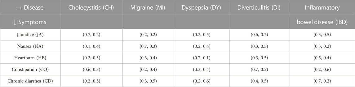
TABLE 1. Symptoms–diseases VR.

TABLE 2

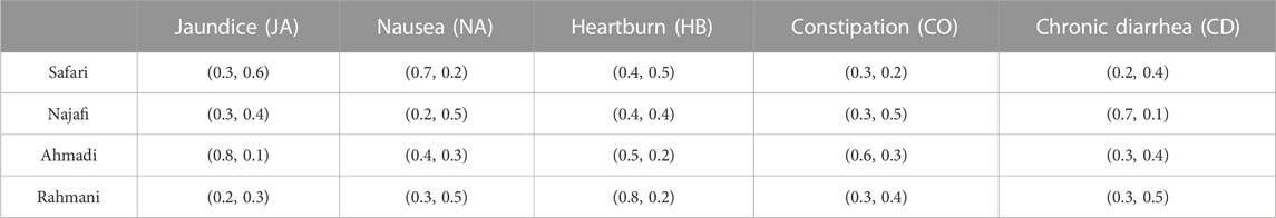
TABLE 2. Patient–symptoms VR.

Now, we show the patients and symptoms as VSs as follows:

$\begin{matrix} C H = {⟨ J A, (0.7, 0.2) ⟩, ⟨ N A, (0.1, 0.4) ⟩, ⟨ H B, (0.2, 0.3) ⟩, ⟨ C O, (0.6, 0.3) ⟩, ⟨ C D, (0.2, 0.3) ⟩} \\ M I = {⟨ J A, (0.2, 0.2) ⟩, ⟨ N A, (0.7, 0.3) ⟩, ⟨ H B, (0.3, 0.4) ⟩, ⟨ C O, (0.2, 0.4) ⟩, ⟨ C D, (0.3, 0.5) ⟩} \\ D Y = {⟨ J A, (0.2, 0.5) ⟩, ⟨ N A, (0.2, 0.4) ⟩, ⟨ H B, (0.7, 0.1) ⟩, ⟨ C O, (0.3, 0.4) ⟩, ⟨ C D, (0.2, 0.6) ⟩} \\ D I = {⟨ J A, (0.6, 0.2) ⟩, ⟨ N A, (0.3, 0.5) ⟩, ⟨ H B, (0.3, 0.5) ⟩, ⟨ C O, (0.7, 0.2) ⟩, ⟨ C D, (0.4, 0.5) ⟩} \\ I B D = {⟨ J A, (0.3, 0.5) ⟩, ⟨ N A, (0.3, 0.2) ⟩, ⟨ H B, (0.5, 0.4) ⟩, ⟨ C O, (0.2, 0.6) ⟩, ⟨ C D, (0.7, 0.2) ⟩} . \end{matrix}$

$\begin{matrix} S a f a r i = {〈 J A, (0.3, 0.6) 〉, 〈 N A, (0.7, 0.2) 〉, 〈 H B, (0.4, 0.5) 〉, 〈 C O, (0.3, 0.2) 〉, 〈 C D, (0.2, 0.4) 〉} \\ N a j a f i = {〈 J A, (0.3, 0.4) 〉, 〈 N A, (0.2, 0.5) 〉, 〈 H B, (0.4, 0.4) 〉, 〈 C O, (0.3, 0.5) 〉, 〈 C D, (0.7, 0.1) 〉} \\ A h m a d i = {〈 J A, (0.8, 0.1) 〉, 〈 N A, (0.4, 0.3) 〉, 〈 H B, (0.5, 0.2) 〉, 〈 C O, (0.6, 0.3) 〉, 〈 C D, (0.3, 0.4) 〉} \\ R a h m a n i = {〈 J A, (0.2, 0.3) 〉, 〈 N A, (0.3, 0.5) 〉, 〈 H B, (0.8, 0.2) 〉, 〈 C O, (0.3, 0.4) 〉, 〈 C D, (0.3, 0.5) 〉} . \end{matrix}$

Here, we calculate the vague distance between the disease and the patients based on their symptoms.

$\begin{matrix} d (C H, S a f a r i) = \frac{2}{5} \{\frac{\sin \frac{π}{6} | 0.7 - 0.3 | + \sin \frac{π}{6} | 0.2 - 0.6 |}{1 + \sin \frac{π}{6} | 0.7 - 0.3 | + \sin \frac{π}{6} | 0.2 - 0.6 |} \\ + \frac{\sin \frac{π}{6} | 0.1 - 0.7 | + \sin \frac{π}{6} | 0.4 - 0.2 |}{1 + \sin \frac{π}{6} | 0.1 - 0.7 | + \sin \frac{π}{6} | 0.4 - 0.2 |} \\ + \frac{\sin \frac{π}{6} | 0.2 - 0.4 | + \sin \frac{π}{6} | 0.3 - 0.5 |}{1 + \sin \frac{π}{6} | 0.2 - 0.4 | + \sin \frac{π}{6} | 0.3 - 0.5 |} \\ + \frac{\sin \frac{π}{6} | 0.6 - 0.3 | + \sin \frac{π}{6} | 0.3 - 0.2 |}{1 + \sin \frac{π}{6} | 0.6 - 0.3 | + \sin \frac{π}{6} | 0.3 - 0.2 |} \\ + \frac{\sin \frac{π}{6} | 0.2 - 0.2 | + \sin \frac{π}{6} | 0.3 - 0.4 |}{1 + \sin \frac{π}{6} | 0.2 - 0.2 | + \sin \frac{π}{6} | 0.3 - 0.4 |}\} \\ = \frac{2}{5} \{0.2875 + 0.2857 + 0.1666 + 0.1666 + 0.0476\} = 0.3808 . \end{matrix}$

$\begin{matrix} d (C H, N a j a f i) = \frac{2}{5} \{\frac{\sin \frac{π}{6} | 0.7 - 0.3 | + \sin \frac{π}{6} | 0.2 - 0.4 |}{1 + \sin \frac{π}{6} | 0.7 - 0.3 | + \sin \frac{π}{6} | 0.2 - 0.4 |} \\ + \frac{\sin \frac{π}{6} | 0.1 - 0.2 | + \sin \frac{π}{6} | 0.4 - 0.5 |}{1 + \sin \frac{π}{6} | 0.1 - 0.2 | + \sin \frac{π}{6} | 0.4 - 0.5 |} \\ + \frac{\sin \frac{π}{6} | 0.2 - 0.4 | + \sin \frac{π}{6} | 0.3 - 0.4 |}{1 + \sin \frac{π}{6} | 0.2 - 0.4 | + \sin \frac{π}{6} | 0.3 - 0.4 |} \\ + \frac{\sin \frac{π}{6} | 0.6 - 0.3 | + \sin \frac{π}{6} | 0.3 - 0.5 |}{1 + \sin \frac{π}{6} | 0.6 - 0.3 | + \sin \frac{π}{6} | 0.3 - 0.5 |} \\ + \frac{\sin \frac{π}{6} | 0.2 - 0.7 | + \sin \frac{π}{6} | 0.3 - 0.1 |}{1 + \sin \frac{π}{6} | 0.2 - 0.7 | + \sin \frac{π}{6} | 0.3 - 0.1 |}\} \\ = \frac{2}{5} \{0.2307 + 0.0909 + 0.1304 + 0.2 + 0.2592\} = 0.3644 . \end{matrix}$

$\begin{matrix} d (C H, A h m a d i) = \frac{2}{5} \{\frac{\sin \frac{π}{6} | 0.7 - 0.8 | + \sin \frac{π}{6} | 0.2 - 0.1 |}{1 + \sin \frac{π}{6} | 0.7 - 0.8 | + \sin \frac{π}{6} | 0.2 - 0.1 |} \\ + \frac{\sin \frac{π}{6} | 0.1 - 0.4 | + \sin \frac{π}{6} | 0.4 - 0.3 |}{1 + \sin \frac{π}{6} | 0.1 - 0.4 | + \sin \frac{π}{6} | 0.4 - 0.3 |} \\ + \frac{\sin \frac{π}{6} | 0.2 - 0.5 | + \sin \frac{π}{6} | 0.3 - 0.2 |}{1 + \sin \frac{π}{6} | 0.2 - 0.5 | + \sin \frac{π}{6} | 0.3 - 0.2 |} \\ + \frac{\sin \frac{π}{6} | 0.6 - 0.6 | + \sin \frac{π}{6} | 0.3 - 0.3 |}{1 + \sin \frac{π}{6} | 0.6 - 0.6 | + \sin \frac{π}{6} | 0.3 - 0.3 |} \\ + \frac{\sin \frac{π}{6} | 0.2 - 0.3 | + \sin \frac{π}{6} | 0.3 - 0.4 |}{1 + \sin \frac{π}{6} | 0.2 - 0.3 | + \sin \frac{π}{6} | 0.3 - 0.4 |}\} \\ = \frac{2}{5} \{0.0909 + 0.1666 + 0.1666 + 0.0909\} = 0.206 . \end{matrix}$

$\begin{matrix} d (C H, R a h m a n i) = \frac{2}{5} \{\frac{\sin \frac{π}{6} | 0.7 - 0.2 | + \sin \frac{π}{6} | 0.2 - 0.3 |}{1 + \sin \frac{π}{6} | 0.7 - 0.2 | + \sin \frac{π}{6} | 0.2 - 0.3 |} \\ + \frac{\sin \frac{π}{6} | 0.1 - 0.3 | + \sin \frac{π}{6} | 0.4 - 0.5 |}{1 + \sin \frac{π}{6} | 0.1 - 0.3 | + \sin \frac{π}{6} | 0.4 - 0.5 |} \\ + \frac{\sin \frac{π}{6} | 0.2 - 0.8 | + \sin \frac{π}{6} | 0.3 - 0.2 |}{1 + \sin \frac{π}{6} | 0.2 - 0.8 | + \sin \frac{π}{6} | 0.3 - 0.2 |} \\ + \frac{\sin \frac{π}{6} | 0.6 - 0.3 | + \sin \frac{π}{6} | 0.3 - 0.4 |}{1 + \sin \frac{π}{6} | 0.6 - 0.3 | + \sin \frac{π}{6} | 0.3 - 0.4 |} \\ + \frac{\sin \frac{π}{6} | 0.2 - 0.3 | + \sin \frac{π}{6} | 0.3 - 0.5 |}{1 + \sin \frac{π}{6} | 0.2 - 0.3 | + \sin \frac{π}{6} | 0.3 - 0.5 |}\} \\ = \frac{2}{5} \{0.2307 + 0.1304 + 0.2592 + 0.1666 + 0.1304\} = 0.3669 . \end{matrix}$

In the same way, we have

$\begin{matrix} d (M I, S a f a r i) = 0.2239, d (M I, N a j a f i) = 0.3255 \\ d (M I, A h m a d i) = 0.3215, d (M I, R a h m a n i) = 0.2340, \\ d (D Y, S a f a r i) = 0.3164, d (D Y, N a j a f i) = 0.300, \\ d (D Y, A h m a d i) = 0.3564, d (D Y, R a h m a n i) = 0.1454, \\ d (D I, S a f a r i) = 0.3452, d (D I, N a j a f i) = 0.3427, \\ d (D I, A h m a d i) = 0.2570, d (D I, R a h m a n i) = 0.3056, \\ d (I B D, S a f a r i) = 0.3057, d (I B D, N a j a f i) = 0.1601, \\ d (I B D, A h m a d i) = 0.3928, d (I B D, R a h m a n i) = 0.3401 . \end{matrix}$

The distance matrix for the aforementioned values is as follows:

$\begin{matrix} \begin{matrix} S a f a r i & N a j a f i & A h m a d i & R a h m a n i \end{matrix} \\ \begin{matrix} C h o l e c y s t i t i s \\ M i g r a i n e \\ D y s p e p s i a \\ D i v e r t i c u l i t i s \\ I n f l a m m a t o r y b o w l d i s e a s e \end{matrix} (\begin{matrix} 0.3808 & 0.3644 & 0.206 & 0.3669 \\ 0.2239 & 0.3255 & 0.3215 & 0.3240 \\ 0.3164 & 0.300 & 0.3564 & 0.1454 \\ 0.3452 & 0.3427 & 0.2570 & 0.3056 \\ 0.3057 & 0.1601 & 0.3928 & 0.3401 \end{matrix}) \end{matrix}$

As the distance between the patient and the mentioned diseases decreases, the probability of the patient suffering from that disease increases, so we conclude that Safari suffers from migraine, Najafi suffers from inflammatory bowel disease, Ahmadi suffers from cholecystitis, and Rahmani suffers from dyspepsia.

5 Conclusion

VGs are important in other sciences, including psychology, life sciences, medicine, and social studies, and can help researchers with optimization and save time and money. Likewise, VGs, belonging to the FG family, have good abilities because they face problems that cannot be explained by FGs. Hence, in this study, we introduced the notion of VEG and presented some of its properties. Moreover, we characterized VG ζ = (M, N), where M is a VS and N is a VR. Some operations have been defined, such as CP, cross product, LP, and SP on VGs. Finally, an application of VG in medical sciences has been presented. In our future work, we will introduce some connectivity indices, such as the Wiener index, harmonic index, Zagreb index, and Randic index in VGs, and investigate some of their properties.

Data availability statement

The original contributions presented in the study are included in the article/Supplementary Material. Further inquiries can be directed to the corresponding author.

Author contributions

All authors have made a substantial, direct, and intellectual contribution to the work and approved it for submission.

Funding

This work was supported by the National Key R and D Program of China (Grant 2019YFA0706 338402) and the National Natural Science Foundation of China under grants 62172302, 62072129, and 61876047.

Conflict of interest

The authors declare that the research was conducted in the absence of any commercial or financial relationships that could be construed as a potential conflict of interest.

Publisher’s note

All claims expressed in this article are solely those of the authors and do not necessarily represent those of their affiliated organizations, or those of the publisher, the editors, and the reviewers. Any product that may be evaluated in this article, or claim that may be made by its manufacturer, is not guaranteed or endorsed by the publisher.

References

1. Zadeh LA. Fuzzy sets. Fuzzy sets, Inf Control (1965) 8:338–53. doi:10.1016/s0019-9958(65)90241-x

CrossRef Full Text | Google Scholar

2. Gau WL, Buehrer DJ. Vague sets. IEEE Trans Syst Man, Cybernetics (1993) 23(2):610–4. doi:10.1109/21.229476

CrossRef Full Text | Google Scholar

3. Kauffman A. Introduction a la theories des sous-emsembles 503 ous. Masson Cie (1973) 1:607–18.

Google Scholar

4. Zadeh LA. Similarity relations and fuzzy orderings. Inf Sci (1971) 3:177–200. doi:10.1016/s0020-0255(71)80005-1

CrossRef Full Text | Google Scholar

5. Zadeh LA. Is there a need for fuzzy logical. Inf Sci (2008) 178:2751–79. doi:10.1016/j.ins.2008.02.012

CrossRef Full Text | Google Scholar

6. Rosenfeld A. In: LA Zadeh, KS Fu, and M Shimura, editors. Fuzzy graphs, fuzzy sets and their applications. New York, NY, USA: Academic Press (1975). p. 77–95.

CrossRef Full Text | Google Scholar

7. Mordeson JN, Chang-Shyh P. Operations on fuzzy graphs. Inf Sci (1994) 79:159–70. doi:10.1016/0020-0255(94)90116-3

CrossRef Full Text | Google Scholar

8. Ghorai G, Pal M. Certain types of product bipolar fuzzy graphs. Int J Appl Comput Math (2017) 3(2):605–19. doi:10.1007/s40819-015-0112-0

CrossRef Full Text | Google Scholar

9. Ghorai G, Pal M. On some operations and density of m-polar fuzzy graphs. Pac Sci Rev A: Nat Sci Eng (2015) 17(1):14–22. doi:10.1016/j.psra.2015.12.001

CrossRef Full Text | Google Scholar

10. Das K, Samanta S, De K. Generalized neutrosophic competition graphs. Neutrosophic Sets Syst (2020) 31:156–71.

Google Scholar

11. Bhattacharya P. Some remarks on fuzzy graphs. Pattern Recognition Lett (1987) 6(5):297–302. doi:10.1016/0167-8655(87)90012-2

CrossRef Full Text | Google Scholar

12. Mordeson JN, Nair PS. Fuzzy graphs and fuzzy hypergraphs. 2nd ed. Physica, Heidelberg, Germany: Springer (2001).

Google Scholar

13. Mahapatra R, Samanta S, Allahviranloo T, Pal M. Radio fuzzy graphs and assignment of frequency in radio stations. Comput Appl Math (2019) 38(3):117–20. doi:10.1007/s40314-019-0888-3

CrossRef Full Text | Google Scholar

14. Akram M, Gani N, Borumand Saeid A. Vague hyper graphs. J Int Fuzzy Syst (2014) 26:647–53. doi:10.3233/ifs-120756

CrossRef Full Text | Google Scholar

15. Akram M, Samanta S, Pal M. Cayley vague graphs. J Fuzzy Math (2017) 25(2):1–14.

Google Scholar

16. Akram M, Feng F, Sarwar S, Jun YB. Certain types of vague graphs. U.P.B Sci Bull Ser A (2014) 76(1):141–54.

Google Scholar

17. Rashmanlou H, Samanta S, Pal M, Borzooei RA. A study on vague graphs. SpringerPlus (2016) 5(1):1234–12. doi:10.1186/s40064-016-2892-z

PubMed Abstract | CrossRef Full Text | Google Scholar

18. Samanta S, Pal M, Rashmanlou H, Borzooei RA. Vague graphs and strengths. J Intell Fuzzy Syst (2016) 30(6):3675–80. doi:10.3233/ifs-162113

CrossRef Full Text | Google Scholar

19. Samanta S, Pal M, Mahapatra R, Das K, Singh Bhadoria R. A study on semi-directed graphs for social media networks. Int J Comput Intelligence Syst (2021) 14(1):1034–41. doi:10.2991/ijcis.d.210301.001

CrossRef Full Text | Google Scholar

20. Samanta S, Kumar Dubey V, Sarkar B. Measure of influences in social networks. Appl Soft Comput (2021) 99:106858. doi:10.1016/j.asoc.2020.106858

CrossRef Full Text | Google Scholar

21. Shoaib M, Kosari S, Rashmanlou H, Aslam Malik M, Rao Y, Talebi Y, et al. Notion of complex pythagorean fuzzy graph with properties and application. J Multiple-Valued Logic Soft Comput (2020) 34:553–86.

Google Scholar

22. Ramakrishna N. Vague graphs. Int J Cogn Comput (2009) 7:51–8.

Google Scholar

23. Borzooei RA, Rashmanlou H. Domination in vague graphs and its applications. J Intell Fuzzy Syst (2015) 29:1933–40. doi:10.3233/IFS-151671

CrossRef Full Text | Google Scholar

24. Borzooei RA, Rashmanlou H. Degree of vertices in vague graphs. J Appl Math Inform (2015) 33(5):545–57. doi:10.14317/jami.2015.545

CrossRef Full Text | Google Scholar

25. Sunitha MS, Vijayakumar A. Complement of a fuzzy graph. Indian J Pure Appl Math (2002) 33:1451–64.

Google Scholar

26. Kosari S, Rao Y, Jiang H, Liu X, Wu P, Shao Z. Vague graph Structure with Application in medical diagnosis. Symmetry (2020) 12(10):1582. doi:10.3390/sym12101582

CrossRef Full Text | Google Scholar

27. Kou Z, Kosari S, Akhoundi M. A novel description on vague graph with application in transportation systems. J Math (2021) 2021:4800499. doi:10.1155/2021/4800499

CrossRef Full Text | Google Scholar

28. Rao Y, Kosari S, Shao Z. Certain Properties of vague Graphs with a novel application. Mathematics (2020) 8(10):1647. doi:10.3390/math8101647

CrossRef Full Text | Google Scholar

29. Rao Y, Kosari S, Shao Z, Cai R, Xinyue L. A Study on Domination in vague incidence graph and its application in medical sciences. Symmetry (2020) 12(11):1885. doi:10.3390/sym12111885

CrossRef Full Text | Google Scholar

30. Rao Y, Kosari S, Shao Z, Qiang X, Akhoundi M, Zhang X. Equitable domination in vague graphs with application in medical sciences. Front Phys (2021) 9:635642. doi:10.3389/fphy.2021.635642

CrossRef Full Text | Google Scholar

31. Shi X, Kosari S. Certain properties of domination in product vague graphs with an application in medicine. Front Phys (2021) 9:680634. doi:10.3389/fphy.2021.680634

CrossRef Full Text | Google Scholar

32. Shao Z, Kosari S, Rashmanlou H, Shoaib M. New concepts in intuitionistic fuzzy graph with application in water supplier systems. Mathematics (2020) 8(8):1241. doi:10.3390/math8081241

CrossRef Full Text | Google Scholar

Keywords: vague set, vague edge graph, (λ, δ)-level graph, lexicographic product, cross product, strong product

Citation: Shi X, Jiang W, Khan A and Akhoundi M (2023) New concepts on level graphs of vague graphs with application in medicine. Front. Phys. 11:1130765. doi: 10.3389/fphy.2023.1130765

Received: 23 December 2022; Accepted: 18 January 2023;
Published: 21 February 2023.

Edited by:

Yilun Shang, Northumbria University, United Kingdom

Reviewed by:

Sovan Samanta, Tamralipta Mahavidyalaya, India
Madhumangal Pal, Vidyasagar University, India

Copyright © 2023 Shi, Jiang, Khan and Akhoundi. This is an open-access article distributed under the terms of the Creative Commons Attribution License (CC BY). The use, distribution or reproduction in other forums is permitted, provided the original author(s) and the copyright owner(s) are credited and that the original publication in this journal is cited, in accordance with accepted academic practice. No use, distribution or reproduction is permitted which does not comply with these terms.

*Correspondence: Wubian Jiang, jwb65659@163.com

Disclaimer: All claims expressed in this article are solely those of the authors and do not necessarily represent those of their affiliated organizations, or those of the publisher, the editors and the reviewers. Any product that may be evaluated in this article or claim that may be made by its manufacturer is not guaranteed or endorsed by the publisher.