 Gaizhu Qu
 Mengmeng Wang2
- 1School of Mathematics and Physics, Weinan Normal University, Weinan, China
- 2Department of Mathematics, Hangzhou Zhongce Vocational School Qiantang, Hangzhou, China
- 3Department of Applied Mathematics, Zhejiang University of Technology, Hangzhou, China
We extend the invariant subspace method (ISM) to a class of Hamilton–Jacobi equations (HJEs) and a family of third-order time-fractional dispersive PDEs with the Caputo fractional derivative in this letter. More precisely, the complete classification is presented for such HJEs that admit invariant subspaces governed by solutions of the second-order and third-order linear ordinary differential equations (ODEs). Meanwhile, some concrete equations are derived for the construction of new exact solutions
1 Introduction
One of the recently invented methods to derive the explicit solution of NPDE is ISM, which was initiated by Galaktionov and Svirshchevskii in [1] and many researchers have illustrated its applicability in Refs. [2–6]. Specifically, Refs. [2, 3, 5, 6] have addressed the basic question of the dimension of invariant subspaces, which in addition to ISM is also relevant to Lie-B
In this paper, we analyze the following two families of special-type non-linear evolution equations.
1.1 Hamilton–Jacobi equations
Hamilton–Jacobi equations (HJEs) can be regarded as models for various processes in theoretical physics, quantum mechanics and contemporary problems of control, etc. In Refs. [24–28], the authors analyzed HJEs in different directions. References [29–32] have also indicated that these equations can be used to depict several properties including blow up behavior and the long time action of non-linear diffusion equations. We will consider the following HJEs
where u = u(t, x) and p(x), B(u), Q(x, u) are sufficiently smooth functions of indicated variables. Here we suppose that m ≠ − 1, −2. This assumption means that Eq. 1.1 is a fully non-linear HJE. In Ref. [7], Qu showed that Eq. 1.1 preserves the second-order CLBS with
1.2 Third-order time-fractional dispersive PDEs
The concept of fractional order derivative was initiated with the half-order derivative as considered by Leibniz and L’Hopital and many authors have generalized it to an arbitrary order derivative. Different concepts of fractional derivatives were proposed in [33–36]. Now fNPDEs have gained much attention because they can be utilized to represent a large number of physical processes. Some techniques have been employed to solve fNPDEs, but the study of fNPDEs has been still handicapped due to the limitations on dealing with more complex fNODEs.
We will study a family of third-order time-fractional dispersive PDEs
where u = u(t, x), 0 < α ≤ 1, t > 0, and
If
If α = δ2 = 2b2 = b3 = 1, σ = γ = b1 = 0, Eq. 1.2 becomes the Hunter-Saxton equation [1]:
These equations arise as asymptotic models in the theory of shallow water waves. Many authors have concentrated on studying the above special cases of Eq. 1.2.
The major contents of this paper are as follows. We recall the method of the invariant subspace, and also introduce several definitions and fundamental theorems on fractional derivatives and integrals in Section 2. In Section 3 we obtain the complete invariant subspace classification of Eq. 1.1 and derive the reductions and explicit solutions of several examples by utilizing ISM. In Section 4, combined with LTM and inspired by several properties of the well known ML function, we investigate exact solutions of different cases for Eq. 1.2. In the last section, we make some concluding remarks.
2 Preliminaries
First, we introduce ISM. Then, we give several definitions and properties.
2.1 Invariant subspace method
Now, we will present brief details of ISM for a kth-order NPDE
where
In [15], Gazizov and Kasatkin demonstrated that ISM can be used to reduce a fNPDE to a system of fNODEs.
We focus on the fNPDE of the form
where
Definition 2.1. If differential operator F satisfies F[Wn] ⊆ Wn, the subspace Wn is invariant under F.Let us suppose Eq. 2.2 preserves the subspace Wn, then
{Ci(t), (i = 1, 2, …, n)} satisfy the n-dimensional dynamical system
Observing that the subspace Wn is determined by a basic solution set of a linear nth-order ODE,
Therefore, the invariant condition F is
2.2 Some results on fractional calculus
Definition 2.2. The Riemann–Liouville fractional integral operator of order α > 0 is represented as the following expression:
Where
Definition 2.3. The Caputo fractional differential operator of order α > 0 is represented as the following expression:
When
When α ∈ (0, 1], the LT of Caputo fractional derivative has the following expression
where
Definition 2.4. A ML function is
Also, Eα,1(z) = Eα(z).We can see the γth order Caputo derivatives of the ML function are:
3 Exact solutions of HJEs
3.1 Invariant subspace classification of Eq. 1.1
For Eq. 1.1, we write it in the form
We investigate n = 2 first. After a straightforward calculation, we obtain that
where Ji(i = 1, 2, …, 8) have the following expressions:
Observing the above expression Eq. 3.1, we shall discuss four possibilities: m = −3, 1, 2 and m ≠ − 3, 1, 2. For the case of m = −3, we derive the following system
From the first equation of Eq. 3.3, it is apparent that B(u) = b1u + b2. By solving the fifth and sixth equations of Eq. 3.3, we obtain Q(x, u) = q1u + Q1(x), where b1, b2 and q1 are arbitrary constants and Q1(x) is a function of x. Inserting B(u) = b1u + b2 and Q(x, u) = q1u + Q1(x) into system Eq. 3.3, we have
Taking into account the assumption p(x) ≠ 0 and solving the system (3.4), the corresponding classifying equations and two-dimensional invariant subspaces are listed as the first three lines in Table 1 with the case m = −3. The cases of m = 1, 2 and m ≠ − 3, 1, 2 can be dealt in a similar way; therefore, we obtain the invariant subspace classification results, which are presented in Table 1.
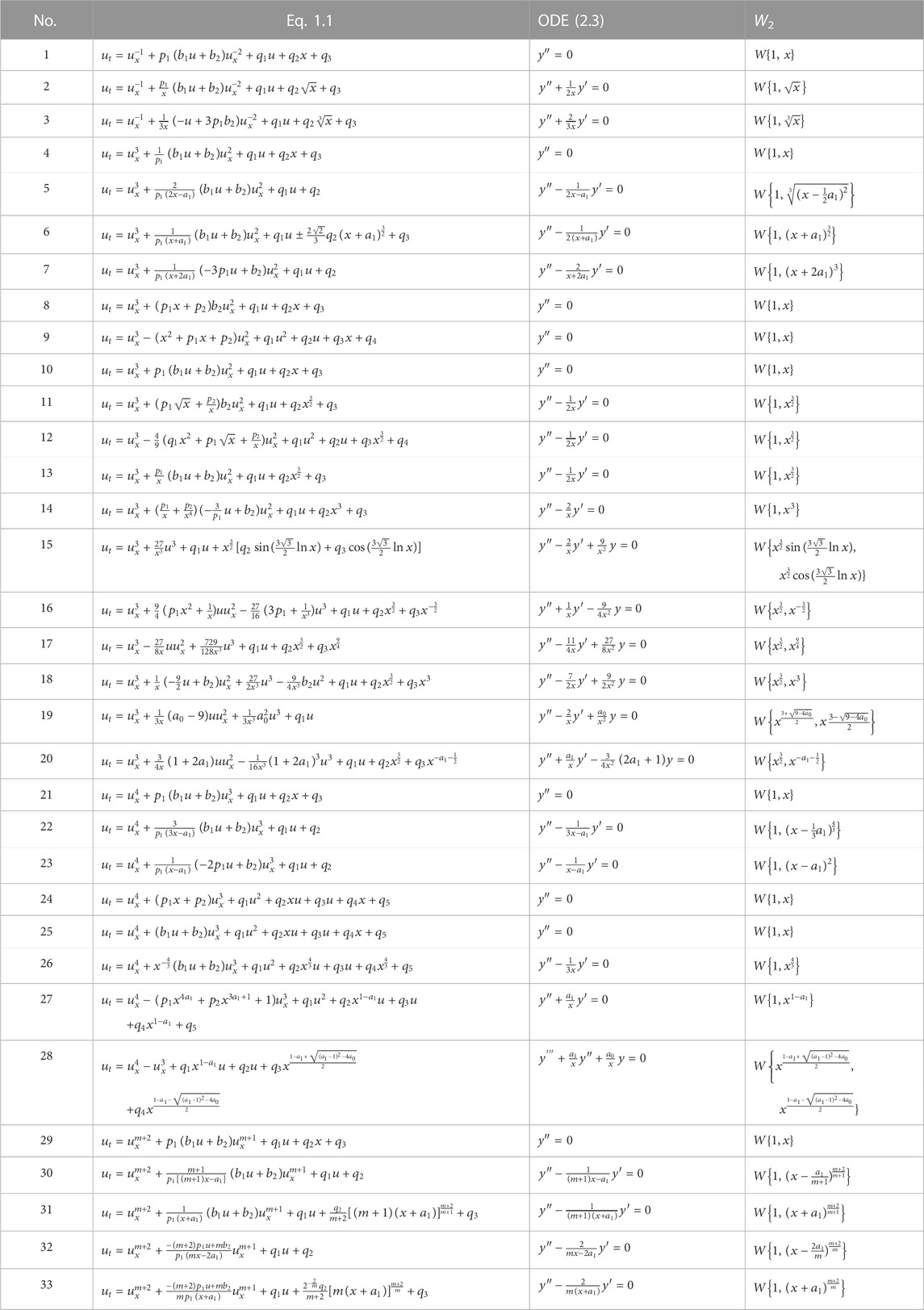
TABLE 1. Classifications of W2 governed by linear ODEs (2.3) of Eq. 1.1.
When n = 3, we find there is only one case: m = 0, and the corresponding results are listed in Table 2.
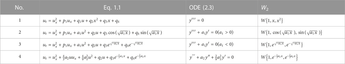
TABLE 2. Classifications of W3 governed by linear ODEs (2.3) of Eq. 1.1.
3.2 Applications
In this section, we provide a further discussion for addressing with the explicit solutions using the above classification results.
Example 1: The equation
admits the two-dimensional invariant subspace
As a result, we derive that
Substituting the above solution into Eq. 3.5, we obtain
For q1 = 0, we can see that
For q1 ≠ 0, we have
The corresponding solution shown in Figure 1
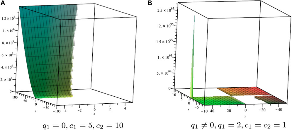
FIGURE 1. Solution profile of Eq. 3.5.
Example 2: The equation
admits the invariant subspace
Then, we arrive at
Inserting the above solution into Eq. 3.6, we obtain
For q1 = 0, we obtain
For q1 ≠ 0, we have
The corresponding solution shown in Figure 2
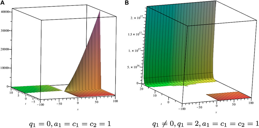
FIGURE 2. Solution profile of Eq. 3.6.
Example 3: The equation
admits the two-dimensional invariant subspace
Then we arrive at
Inserting the above solution into Eq. 3.7, we obtain
we can see that
The corresponding solution shown in Figure 3
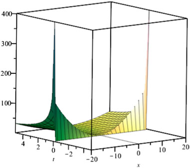
FIGURE 3. Solution profile of Eq. 3.7 with m = 2, c1 = c2 = 1.
Example 4: The equation
admits the three-dimensional trigonometric invariant subspace
Then we arrive at
Inserting the above solution into Eq. 3.8, we obtain
For q2 = 0, we can see that
For q2 ≠ 0, we have
The corresponding solution shown in Figure 4
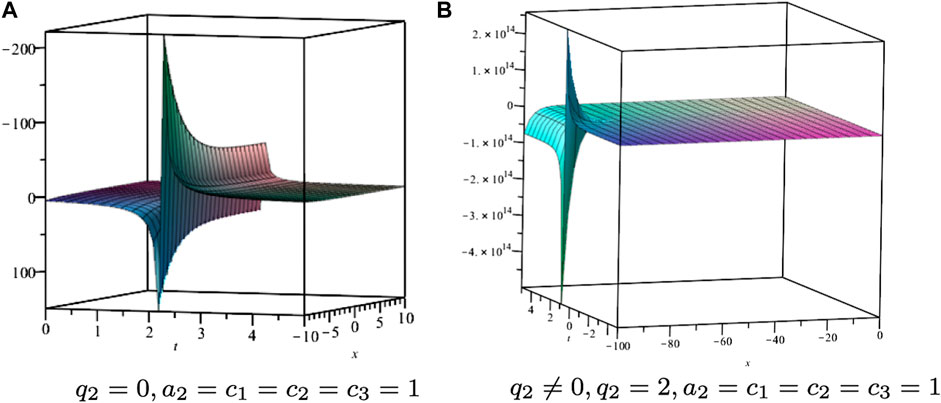
FIGURE 4. Solution profile of Eq. 3.8.
4 Exact solutions of a family of third-order time-fractional dispersive PDEs
Now, we will investigate the different invariant subspaces of non-linear differential operator F[u] and discuss explicit solutions of Eq. 1.2, see the following discussions.
Case 1. Let us consider the following equation
Here
This means that Eq. 4.1 has the following explicit solution:
Substituting the solution into Eq. 4.1, we have
and
Then
The corresponding solution shown in Figure 5
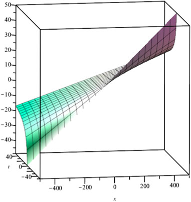
FIGURE 5. Solution profile of Eq. 4.1 with α = 1/3, b1 = 2.
Case 2. We consider the equation
α ∈ (0, 1], Eq. 4.4 preserves invariant subspace
which means that Eq. 4.4 has the solution
Plugging the solution into Eq. 4.4, we find
Solving Eq. 4.5, C1(t) = c1, c1 is an arbitrary constant, and when
Therefore, Eq. 4.6 becomes
Applying the LT to Eq. 4.7, we have
namely,
Here C2(0) = a, its inverse LT is
where Eα,1(.) is the ML function
Hence, we derive that
In the case of α = 1, it is a traveling wave solution
The corresponding solution shown in Figure 6
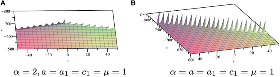
FIGURE 6. Solution profile of Eq. 4.4.
Case 3. We consider the equation
α ∈ (0, 1], Eq. 4.8 admits the two-dimensional invariant subspace
This indicates that Eq. 4.8 has the solution
Substituting the solution into Eq. 4.8, we have
Here,
Now we discuss the following Cauchy problem:
Then, define
At the same time, applying LT to the first equation of Eq. 4.11, we obtain
Inserting Eq. 4.12 into Eq. 4.13, we find
whose inverse LT is
where E2α,1(.) is the ML function
Substituting Eq. 4.14 in Eq. 4.10, we get
By applying Iα on both sides of Eq. 4.15, we obtain
For the sake of simplicity, we set the integration constant to zero. Assuming a = 1, the solution of Eq. 4.8 is
Note that for α = 1,
and the solution becomes
The corresponding solution shown in Figure 7
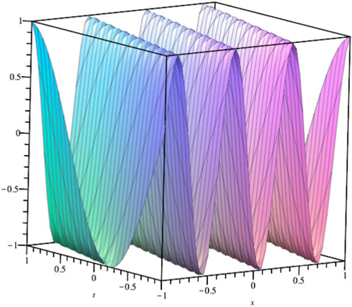
FIGURE 7. Solution profile of Eq. 4.8 with a0 = 100, σ = γ = 1, δ = 2.
Case 4. We consider the equation
α ∈ (0, 1], Eq. 4.16 admits the two-dimensional invariant subspace
This means that the explicit solution has the following form
Substituting the solution into Eq. 4.16, we have
where
Its inverse LT is
Utilizing C1(t) in Eq. 4.18, we obtain
However, while the ML function does not fulfill the following composition property
it should be noted that
which satisfies the composition property, that is,
Thus, we find
Taking Iα on Eq. 4.19 and applying the integration of the ML function relation, we derive the following result:
Here, we set C2(0) = 0. Hence, the exact solution of Eq. 4.16 associated with
Note that for α = 1,
The corresponding solution shown in Figure 8
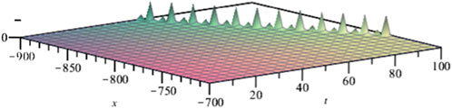
FIGURE 8. Solution profile of Eq. 4.16 with a1 = 1, λ1 = 1, λ2 = 2, δ = 2.
Case 5. We consider the equation
α ∈ (0, 1], Eq. 4.20 admits the three-dimensional invariant subspace
This means that the exact solution has the following form:
Substituting the solution into Eq. 4.20, we obtain
Solving Eq. 4.21, we obtain C1(t) = c1, inserting it into Eq. 4.22 and Eq. 4.23, we find
where
Note that for α = 1,
and the solution is
which is a compacton solution.The corresponding solution shown in Figure 9
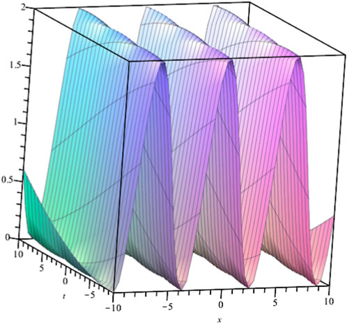
FIGURE 9. Solution profile of Eq. 4.20 with α = γ = b2 = b3 = c1 = 1, δ = 10.
Case 6. We consider the equation
This means that the exact solution has the following form
Substituting the solution into (4.24), we have
Solving this system, we derive that
Thus, Eq. 4.24 has the solution
where
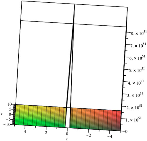
FIGURE 10. Solution profile of Eq. 4.24 with α = 1/3, b2 = b3 = 1, δ = 10.
5 Conclusion
In this work, a class of HJEs (1.1) and a family of third-order time-fractional dispersive PDEs (1.2) are investigated by utilizing ISM. All invariant subspaces for the considered HJEs are derived and displayed in Table 1 and Table 2. Meanwhile, some exact solutions to the equations are obtained due to the corresponding symmetry reductions. For the third-order time-fractional dispersive PDEs, the right-hand side of Eq. 1.2 is the derivative of a quadratic differential polynomial, therefore they preserve more than one invariant subspace, each of which generates a solution. Then, by employing the LT method and applying several properties of the well known ML function, the different kinds of explicit solutions of Eq. 1.2 are derived.
There are still some important problems to be considered. For instance, how does one use ISM to resolve initial value problems? How can we develop this method to investigate higher-dimensional non-linear equations and their discrete versions? This will be considered in the future. Moreover, in the extended version of this work, we will discuss more complicated fractional differential equations by using ISM.
Data availability statement
The original contributions presented in the study are included in the article/supplementary material, further inquiries can be directed to the corresponding authors.
Author contributions
GQ: Investigation, methodology, software, writing—original draft. MW: Writing—review and editing, software. SS: Formal analysis, writing—review and editing, supervision. All authors contributed to the article and approved the submitted version.
Funding
The work was supported by the National Natural Science Foundation of China (Grant No. 11501419), the Natural Science Foundation of Shaanxi Province, China (Grant No. 2021JM-521) and the Key Research Foundation of Weinan City, China (Grant No. 2019ZDYF-JCYJ-118).
Conflict of interest
The authors declare that the research was conducted in the absence of any commercial or financial relationships that could be construed as a potential conflict of interest.
Publisher’s note
All claims expressed in this article are solely those of the authors and do not necessarily represent those of their affiliated organizations, or those of the publisher, the editors and the reviewers. Any product that may be evaluated in this article, or claim that may be made by its manufacturer, is not guaranteed or endorsed by the publisher.
References
1. Galaktionov VA, Svirshchevskii SR. Exact solutions and invariant subspaces of nonlinear partial differential equations in mechanics and physics. London: Chapman and Hall/CRC (2007).
2. Qu CZ, Zhu CR. Classification of coupled systems with two-component nonlinear diffusion equations by the invariant subspace method. J Phys A Math Theor (2009) 42:475201. [27pp]. doi:10.1088/1751-8113/42/47/475201
3. Zhu CR, Qu CZ. Maximal dimension of invariant subspaces admitted by nonlinear vector differential operators. J Math Phys (2011) 52:043507. [15pp]. doi:10.1063/1.3574534
4. Ma WX. A refined invariant subspace method and applications to evolution equations. Sci China Math (2012) 55:1769–78. doi:10.1007/s11425-012-4408-9
5. Song JQ, Shen SF, Jin YY, Zhang J. New maximal dimension of invariant subspaces to coupled systems with two-component equations. Commun Nonlinear Sci Numer Simulat (2013) 18:2984–92. doi:10.1016/j.cnsns.2013.03.019
6. Shen SF, Qu CZ, Jin YY, Ji LN. Maximal dimension of invariant subspaces to systems of nonlinear evolution equations. Chin Ann Math Ser B (2012) 33:161–78. doi:10.1007/s11401-012-0705-4
7. Qu CZ. Conditional Lie Bäcklund symmetries of Hamilton-Jacobi equations. Nonlinear Anal (2009) 71:e243–e258.doi:10.1016/j.na.2008.10.045
8. Svirshchevskii SR. Lie Bäcklund symmetries of linear ODEs and generalized separation of variables in nonlinear equations. Phys Lett A (1995) 99:344–8.
9. King JR. Exact polynomial solutions to some nonlinear diffusion equations. Phys D (1993) 64:35–65. doi:10.1016/0167-2789(93)90248-y
10. Fokas AS, Liu QM. Nonlinear interaction of traveling waves of nonintegrable equations. Phys Rev Lett (1994) 72:3293–6. doi:10.1103/physrevlett.72.3293
11. Zhdanov RZ. Conditional Lie-Bäcklund symmetry and reductions of evolution equations. J Phys A Math Gen (1995) 28:3841–50.
12. Qu CZ. Group classification and generalized conditional symmetry reduction of the nonlinear diffusion-convection equation with a nonlinear source. Stud Appl Math (1997) 99:107–36. doi:10.1111/1467-9590.00058
13. Qu CZ. Exact solutions to nonlinear diffusion equations obtained by a generalized conditional symmetry method. IMA J Appl Math (1999) 62:283–302. doi:10.1093/imamat/62.3.283
14. Ji LN, Qu CZ. Conditional Lie Bäcklund symmetries and solutions to (n+1)-dimensional nonlinear diffusion equationscklund symmetries and solutions to (n + 1)-dimensional nonlinear diffusion equations. J Math Phys (2007) 48:103509. doi:10.1063/1.2795216
15. Gazizov RK, Kasatkin AA. Construction of exact solutions for fractional order differential equations by invariant subspace method. Comput Math Appl (2013) 66:576–84.doi:10.1016/j.camwa.2013.05.006
16. Sahadevan R, Bakkyaraj T. Invariant subspace method and exact solutions of certain nonlinear time fractional partial differential equations. Fract Calc Appl Anal (2015) 18:146–62. doi:10.1515/fca-2015-0010
17. Harris PA, Garra R. Analytic solution of nonlinear fractional Burgers-type equation by invariant subspace method. Nonlinear Stud (2013) 20:471–81. doi:10.48550/arXiv.1306.1942
18. Prakash P, Priyendhu KS, Lakshmanan M. Invariant subspace method for (m+1)-dimensional non-linear time-fractional partial differential equations. Commun Nonlinear Sci Numer Simulat (2022) 111:106436.doi:10.1016/j.cnsns.2022.106436
19. Prakash P, Priyendhu KS, Anjitha KM. Initial value problem for the (2+1)-dimensional time-fractional generalized convection-reaction-diffusion wave equation:invariant subspace and exact solutions. Comput Appl Math (2022) 41:1–55.
20. Sahadevan R, Prakash P. Exact solutions and maximal dimension of invariant subspaces of time fractional coupled nonlinear partial differential equations. Commun Nonlinear Sci Numer Simulat (2017) 42:158–77. doi:10.1016/j.cnsns.2016.05.017
21. Rui WG. Idea of invariant subspace combined with elementary integral method for investigating exact solutions of time-fractional NPDEs. Appl Math Comput (2018) 339:158–71. doi:10.1016/j.amc.2018.07.033
22. Feng W, Zhao SL. Time-fractional inhomogeneous nonlinear diffusion equation: Symmetries, conservation laws, invariant subspaces, and exact solutions. Mod Phys Lett B (2018) 32:1850401. doi:10.1142/s0217984918504018
23. Choudhary S, Prakash P, Varsha DG. Invariant subspaces and exact solutions for a system of fractional PDEs in higher dimensions. Comput Appl Math (2019) 38:126. doi:10.1007/s40314-019-0879-4
24. Crandall MG, Lions PL. Viscosity solutions of Hamilton-Jacobi equations. Trans Amer Math Soc (1983) 277:1–42. doi:10.1090/s0002-9947-1983-0690039-8
25. Crandall MG, Evans LC, Lions PL. Some properties of viscosity solutions of Hamilton-Jacobi equations. Trans Amer Math Soc (1984) 282:487–502. doi:10.1090/s0002-9947-1984-0732102-x
26. Crandall MG, Lions PL. On existence and uniqueness of solutions of Hamilton-Jacobi equations. Nonlinear Anal TMA (1986) 10:353–70. doi:10.1016/0362-546x(86)90133-1
27. Evans LC. Partial differential equations. In: Graduate studies in mathematics. Providence, RI: American Mathematical Society (1998).
28. Wei QL. Viscosity solution of the Hamilton-Jacobi equation by a limiting minimax method. Nonlinearity (2014) 27:17–41. doi:10.1088/0951-7715/27/1/17
29. Galaktionov VA. Gemetric sturmian theory of nonlinear parabolic equations and applications. Boca Raton, FL: Chapman and Hall/CRC (2004).
30. Galaktionov VA. Vẚzquez jl. A stability technique for evolution partial differential equations. In: A dynamical systems approach. Boston, MA: Birkhauser Boston, Inc (2004).
31. Galaktionov VA, Vazquez JL. Blow-up for quasilinear heat equations described by means of nonlinear Hamilton–Jacobi equationszquez JL. Blow-Up for quasilinear heat equations described by means of nonlinear Hamilton-Jacobi equations. J Differential Equations (1996) 127:1–40. doi:10.1006/jdeq.1996.0059
32. Galaktionov VA, Vazquez JL. Geometrical properties of the solutions of one-dimensional nonlinear parabolic equationszquez JL. Geometrical properties of the solutions of one-dimensional nonlinear parabolic equations. Math Ann (1995) 303:741–69. doi:10.1007/bf01461014
33. Podlubny I. Fractional differential equations: An introduction to fractional derivatives, fractional differential equations, to methods of their solution and some of their applications. New York: Academic Press (1999).
35. Miller KS, Ross B. An introduction to the fractional calculus and fractional differential equations. New York: John Wiley and Sons (1993).
36. Kilbas AA, Trujillo JJ, Srivastava HM. Theory and applications of fractional differential equations. Amsterdam: Elseiver (2006).
37. Degasperis A, Holm DD, Hone ANW. A new integrable equation with peakon solutions. Theor Math Phys (2002) 133:1463–74. doi:10.48550/arXiv.nlin/0205023
38. Rui WG, He B, Long Y, Chen C. The integral bifurcation method and its application for solving a family of third-order dispersive PDEs. Nonlinear Anal (2008) 69:1256–67. doi:10.1016/j.na.2007.06.027
39. Johnson RS. Camassa-Holm, Korteweg-de Vries and related models for water waves. J Fluid Mech (2002) 455:63–82. doi:10.1017/s0022112001007224
40. Camassa R, Holm D. An integrable shallow water equation with peaked solitons. Phys Rev Lett (1993) 71:1661–4. doi:10.1103/physrevlett.71.1661
41. Chen C, Tang M. A new type of bounded waves for Degasperis-Procesi equation. Chaos Soliton Fract (2006) 27:698–704. doi:10.1016/j.chaos.2005.04.040
Keywords: exact solution, Hamilton–Jacobi equation, complete classification, invariant subspace method, Laplace transform
Citation: Qu G, Wang M and Shen S (2023) Applications of the invariant subspace method on searching explicit solutions to certain special-type non-linear evolution equations. Front. Phys. 11:1160391. doi: 10.3389/fphy.2023.1160391
Received: 07 February 2023; Accepted: 22 February 2023;
Published: 28 March 2023.
Edited by:
Gangwei Wang, Hebei University of Economics and Business, ChinaCopyright © 2023 Qu, Wang and Shen. This is an open-access article distributed under the terms of the Creative Commons Attribution License (CC BY). The use, distribution or reproduction in other forums is permitted, provided the original author(s) and the copyright owner(s) are credited and that the original publication in this journal is cited, in accordance with accepted academic practice. No use, distribution or reproduction is permitted which does not comply with these terms.
*Correspondence: Gaizhu Qu, cXVnYWl6aHUuaGlAMTYzLmNvbQ==; Shoufeng Shen, bWF0aHNzZkB6anV0LmVkdS5jbg==