 Mubashir Qayyum1
 Hijaz Ahmad
- 1Department of Sciences and Humanities, National University of Computer and Emerging Sciences, Lahore, Pakistan
- 2Section of Mathematics, International Telematic University Uninettuno, Roma, Italy
- 3Operational Research Center in Healthcare, Near East University, Mersin, Turkey
- 4Department of Computer Science and Mathematics, Lebanese American University, Beirut, Lebanon
- 5Department of Statistics and Operations Research, College of Science, King Saud University, Riyadh, Saudi Arabia
Physical phenomena and natural disasters, such as tsunamis and floods, are caused due to dispersive water waves and shallow waves caused by earthquakes. In order to analyze and minimize damaging effects of such situations, mathematical models are presented by different researchers. The Wu–Zhang (WZ) system is one such model that describes long dispersive waves. In this regard, the current study focuses on a non-linear (2 + 1)-dimensional time-fractional Wu–Zhang (WZ) system due to its importance in capturing long dispersive gravity water waves in the ocean. A Caputo fractional derivative in the WZ system is considered in this study. For solution purposes, modification of the homotopy perturbation method (HPM) along with the Laplace transform is used to provide improved results in terms of accuracy. For validity and convergence, obtained results are compared with the fractional differential transform method (FDTM), modified variational iteration method (mVIM), and modified Adomian decomposition method (mADM). Analysis of results indicates the effectiveness of the proposed methodology. Furthermore, the effect of fractional parameters on the given model is analyzed numerically and graphically at both integral and fractional orders. Moreover, Caputo, Caputo–Fabrizio, and Atangana–Baleanu approaches of fractional derivatives are applied and compared graphically in the current study. Analysis affirms that the proposed algorithm is a reliable tool and can be used in higher dimensional fractional systems in science and engineering.
1 Introduction
The study of differential equations (DEs) is a pivotal topic as they capture most of the real-world phenomena, i.e., earthquakes [1, 2], natural gas consumption [3, 4], current flow [5], and cooking [6]. These equations can additionally be characterized into linear and non-linear differential equations. Many important and interesting phenomena like electrical circuits [7, 8], DNA sequencing [9, 10], disease modeling and analysis [11, 12], and food chain models [13, 14] are captured through differential equations. Since the order of a DE describes the nature and scope of the captured phenomena, it is therefore important for researchers to cater fractional-order derivatives for a more general study of the physical aspects of the considered phenomena. Fractional models allow better understanding of model dynamics and facilitate researchers to accurately predict changes in the physical systems. The chaos theory [15], nanotechnology [16], fluid flow [17], cosmology [18], and robotics [19] use differential equations for problem formulation. These equations also frequently appear in many branches of mathematics [20, 21], finance [22], economy [23], and biology [24].
The phrase “fractal” was first created in 1975 by mathematician Benoit Mandelbrot [25]. It is a geometric shape that exhibits the same level of non-regularity on all scales. Fractals are infinite patterns, which we frequently see in nature. Snowflakes, trees, mountains, clouds, and coastlines represent fractals as they are highly uneven at both large and small scales. Many important models including the diffusion model of red ink [26] and thin films [27], the vibration model for a concrete beam [28] and electronic devices [29], and the COVID-19 mathematical model [30] contain fractal geometry. The distinction between fractional and fractal is that the former is a statement of a fractional number, while the latter is a geometric figure that is similar at all scales.
The Wu–Zhang system [31] contains non-linear partial differential equations (PDEs) and deals with the motion of water waves in oceans. In 1996, three sets of model equations were first derived by Wu and Zhang and named the Wu–Zhang system of PDEs [31]. This system is used to customize several harbor and coastal designs. This non-linear (2 + 1)-dimensional fractional system describes shallow water dispersive long gravity waves in two horizontal directions, which are given as
where
In order to solve such highly non-linear fractional systems, many analytical and numerical methodologies are utilized by different researchers. Anjum et al. [44] applied Li–He’s modified homotopy perturbation approach to solve the microelectromechanical system. Baitiche et al. [45] used the monotone iterative method for fractional DEs with non-linearity at the boundary. Do et al. [46] extended Chebyshev wavelets to two-dimensional fractional DEs. Hashemi et al. [47] investigated multi-term FDEs using minimization techniques. Tian and Liu utilized the modified exp-function to fractional PDEs in [48]. Furthermore, to solve complex problems, the enhanced homotopy methods can be found in [49, 50]. In this study, a hybrid algorithm is proposed by mixing the classical homotopy perturbation method [51, 52] with the Laplace transform [53] along with different fractional derivatives (Atangana–Baleanu, Caputo–Fabrizio, and Caputo) for a highly non-linear time-fractional (2 + 1)-dimensional WZ system. In the rest of the paper, Section 2 contains preliminary definitions. Section 3 contains the proposed methodology for handling time-fractional (2 + 1)-dimensional WZ system, whereas proof of convergence and error analysis are given in Section 4. Solution and results and discussion are given in Sections 5 and 6, respectively, while a conclusion is given in Section 7.
2 Basic definitions
Definition 1: For a function
Definition 2: According to [55], one can express the Laplace transform L of the function
Definition 3: The Caputo–Fabrizio’s time-fractional derivative
Definition 4: The Laplace transform L of the Caputo–Fabrizio’s time-fractional derivative
Definition 5: A function
Here,
Definition 6: The Laplace transform L connected with Atangana–Baleanu time-fractional derivative
Here, AB(ζ) is a normalization function.
Definition 7: He’s fractional derivative of a function
Definition 8: The core idea behind the two-scale dimension [58, 59], which commonly arises in the non-linear problem, is that while self-similarity is difficult to uncover in practical applications, fractal structures self-assemble on all scales. Creating models with the two-scale dimension allows for the successful description of various physical events.
Definition 9: A Banach space
3 Hybrid algorithm for (2 + 1)-dimensional time-fractional systems
Consider a (2 + 1)-dimensional, time-fractional system as
that has initial conditions
where the unknown functions
The procedure will start by applying the Laplace transform on (9), which gives
Now, by utilizing the basic definitions given in Section 2, we can find the Laplace transform of the fractional derivative. Definition (2) gives
The homotopy of the system is
where
After substituting Eq. 14 in (13) and then comparing similar coefficients of s, we obtainAt s1
The inverse Laplace transform leads to
At sk
Operating the inverse Laplace transform gives the following:
The approximate solution of the given general time-fractional, (2 + 1)-dimensional PDE system is
Residual errors of the system are
The same procedure can be extended to a system that comprises more than three equations.
4 Convergence and error analysis of the hybrid algorithm for (2 + 1)-dimensional fractional systems
4.1 Convergence
Theorem 1: If a Banach space has
Proof: Let us define the sequence of partial sums of Eq. 19 as Qrn. To demonstrate that Qrn(t, x, y) forms a Cauchy sequence in the Banach space, we can proceed by using
If Qrn and Qrm are partial sums with n ≥ m and n, m ϵ N, then utilization of triangle inequality gives
From Eq. 21, we get
Given 0
Since
Thus, Qrn(t, x, y) is a Cauchy sequence in the Banach space, and hence, the given statement is proved.
4.2 Error estimation
Theorem 1: One can determine the maximum absolute truncation error of the solution (19) for a fractional (2 + 1)-dimensional system (9) by using the following expression:
Proof: From Eq. 23, we have
Since 0
5 Solution and analysis of the time-fractional Wu–Zhang system
Consider the following coupled time-fractional (2 + 1)-dimensional WZ system [39]:
that has the initial conditions
where
Solution: The initial step of the He–Laplace procedure is the application of the Laplace transform on both sides of Eq. 29, which gives
Utilization of the Laplace transform on the Caputo’s time-fractional derivative (2) leads to
We construct homotopies of the aforementioned system as
where
In the next step, we will expand
Substitution of Eq. 36 into Eq. 34 and then comparison of a similar coefficient with respect to p givesthe first-order problem
with the condition
By operating the inverse Laplace transform, the solution at first order is
The second-order problem is
that has the condition
The inverse of the Laplace transform gives
The same procedure is applied for higher-order problems. Thus, the approximate solution at the higher order of the (2 + 1)-dimensional Wu–Zhang system can be obtained by
By replacing the approximate solutions (43) in the given system (29), we obtain residual errors
6 Results and discussion
The objective of this study is to propose a new soliton solution of the non-linear time-fractional Wu–Zhang system. This (2 + 1)-dimensional system describes the phenomena of long dispersive waves. The current section is focused on the numerical and graphical results of the WZ system through a hybrid approach by using homotopy perturbation with the Laplace transform, which is known as the He–Laplace algorithm (method). Initially, solutions are captured through the He–Laplace algorithm, considering the fractional derivative in Caputo sense. The obtained results are then analyzed at both fractional and integral orders. Table 1 depicts the residual error at
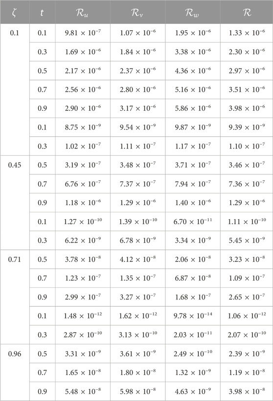
TABLE 1. He–Laplace errors for different values of ζ, when a = d = 0.13, b = 0.11, c = 0.12, x = 3, and y = 6. Here,
Table 2 shows the comparison of results obtained through He–Laplace and other methods at the integer order that is ζ = 1. This numerical comparison indicates that He–Laplace surpasses other mentioned schemes in terms of accuracy. Figure 1 depicts the He–Laplace solution of the WZ system in 3D at the integer order. This graphical illustration confirms that in the WZ system, surface water velocities in x and y directions are very high, while elevation in water waves decreases with time. Error analysis at ζ = 0.4, 0.8, and 1 as 3D structures can be seen from Figure 2 for
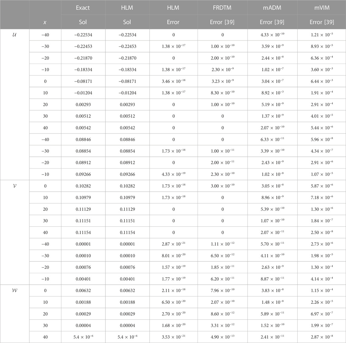
TABLE 2. Error comparison of the He–Laplace algorithm with other methods, when ζ = 1, a = b = 0.1, c = d = 0.01, t = 5, and y = 20.
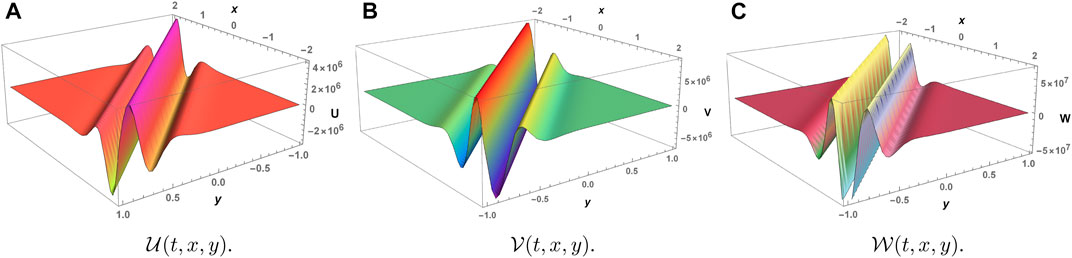
FIGURE 1. Graphical illustration of the He–Laplace solution at ζ = 1, a = c = 2, b = d = 1, and t = 2.
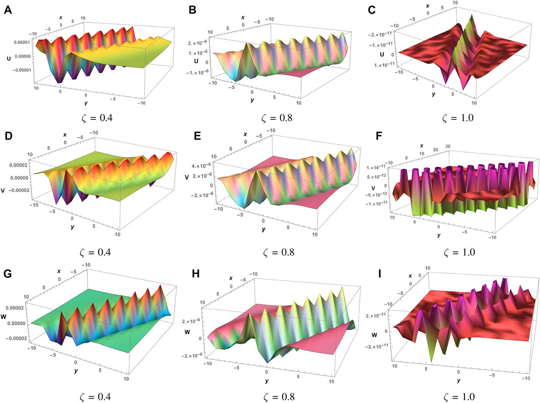
FIGURE 2. Error analysis at different values of the fractional parameter ζ, when a = c = 0.2, b = d = 0.1, and t = 2.
The impact of the fractional parameter on the water surface is depicted in Figure 3. Research findings indicate that a rise in ζ results in a reduction of the water surface velocity, in both the x and y directions. However, water wave elevation
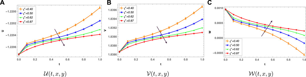
FIGURE 3. Effect of the fractional parameter ζ on the water surface level, when a = 0.8, c = 0.9, b = d = 0.7, y = 3, and x = 2.
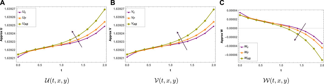
FIGURE 4. Comparison of Caputo, Caputo–Fabrizio, and Atangana–Baleanu fractional derivative approaches on the solution profile, when a = 0.6, b = 0.8, c = 0.9, d = 0.7, y = 2, and x = 5.
7 Conclusion
In this article , a hybrid approach is proposed to solve and analyze the highly non-linear time-fractional (2 + 1)-dimensional WZ system, which is famous for capturing long dispersive waves. A hybrid approach in which homotopy perturbation is combined with the Laplace transform along with different fractional derivatives is proposed for the solution and analysis of the fractional WZ system. Efficiency of the obtained solution is checked over the entire fractional domain to show the validity and convergence of the proposed methodology. Error analysis is also performed in comparison with other well-known numerical methods, which confirms the efficiency of the proposed approach. Graphical analysis shows that water surface velocities increase, while surface elevation decreases, when fractional parameter increases. Also, it is noted that the Atangana–Baleanu approach uplifts water velocities in x and y directions more than Caputo and Caputo–Fabrizio approaches. Analysis of the results also concludes that the proposed method is a reliable technique, which can be extended to more complex fractional systems.
Data availability statement
The original contributions presented in the study are included in the article/Supplementary Material; further inquiries can be directed to the corresponding author.
Author contributions
Conceptualization: MQ. Data curation: EA. Formal analysis: ST. Validation: EA. Writing—original draft: MQ and SS. Writing—review editing: HA and SA. All authors contributed to the article and approved the submitted version.
Funding
This Project is funded by King Saud University, Riyadh, Saudi Arabia.
Acknowledgments
Research Supporting Project number (RSP2023R167), King Saud University, Riyadh, Saudi Arabia.
Conflict of interest
The authors declare that the research was conducted in the absence of any commercial or financial relationships that could be construed as a potential conflict of interest.
Publisher’s note
All claims expressed in this article are solely those of the authors and do not necessarily represent those of their affiliated organizations, or those of the publisher, the editors, and the reviewers. Any product that may be evaluated in this article, or claim that may be made by its manufacturer, is not guaranteed or endorsed by the publisher.
Abbreviations
WZ, Wu–Zhang; DEs, differential equations; PDEs, partial differential equations; FDEs, fractional differential equations; HPM, homotopy perturbation method; HLM, He–Laplace method; mVIM, modified variation iteration method; mADM, modified Adomian decomposition method; FRDTM, fractional reduced differential transform method.
References
1. Dzerjinsky RI. The earthquake attributes disjunctive form analysis at the quickest form change directions. In: Lecture notes in networks and systems. Springer International Publishing (2021). p. 96–101.
2. Hirano S. Source time functions of earthquakes based on a stochastic differential equation. Scientific Rep (2022) 12(1):3936. doi:10.1038/s41598-022-07873-2
3. Zheng C, Wu W-Z, Xie W, Li Q. A MFO-based conformable fractional nonhomogeneous grey Bernoulli model for natural gas production and consumption forecasting. Appl Soft Comput (2021) 99:106891. doi:10.1016/j.asoc.2020.106891
4. Liu C, Wu W-Z, Xie W, Zhang T, Zhang J. Forecasting natural gas consumption of China by using a novel fractional grey model with time power term. Energ Rep (2021) 7(788–797):788–97. doi:10.1016/j.egyr.2021.01.082
5. Akbar MA, Abdul Kayum M, Osman MS, Abdel-Aty A-H, Eleuch H. Analysis of voltage and current flow of electrical transmission lines through mZK equation. Results Phys (2021) 20:103696. doi:10.1016/j.rinp.2020.103696
6. Bidkhori P, Karizaki VM. Diffusion and kinetic modeling of water absorption process during soaking and cooking of chickpea. Legume Sci (2021) 4(1). doi:10.1002/leg3.116
7. Ahmadova A, Mahmudov NI. Langevin differential equations with general fractional orders and their applications to electric circuit theory. J Comput Appl Math (2021) 388:113299. doi:10.1016/j.cam.2020.113299
8. Khader MM, Gómez-Aguilar JF, Adel M. Numerical study for the fractional RL, RC, and RLC electrical circuits using legendre pseudo-spectral method. Int J Circuit Theor Appl (2021) 49(10):3266–85. doi:10.1002/cta.3103
9. Caro LAP, Mendoza R, Mendoza VMP. Application of genetic algorithm with multi-parent crossover on an inverse problem in delay differential equations. In: PROCEEDINGS OF THE INTERNATIONAL CONFERENCE ON MATHEMATICAL SCIENCES AND TECHNOLOGY 2020 (MATHTECH 2020): Sustainable Development of Mathematics and Mathematics in Sustainability Revolution. AIP Publishing (2021).
10. Chen Y, Luo Y, Liu Q, Xu H, Zhang D. Any equation is a forest: Symbolic genetic algorithm for discovering open-form partial differential equations (sga-pde) (2021).
11. Salazar-Viedma M, Gabriel Vergaño-Salazar J, Pastenes L, D’Afonseca V. Simulation model for hashimoto autoimmune thyroiditis disease. Endocrinology (2021) 162(12):bqab190. doi:10.1210/endocr/bqab190
12. Guzzi PH, Petrizzelli F, Mazza T. Disease spreading modeling and analysis: A survey. Brief Bioinform (2022) 23(4). doi:10.1093/bib/bbac230
13. Sahoo D, Samanta GP. Comparison between two tritrophic food chain models with multiple delays and anti-predation effect. Int J Biomath (2021) 14(03). doi:10.1142/s1793524521500108
14. Mondal B, Ghosh U, Rahman MS, Saha P, Sarkar S. Studies of different types of bifurcations analyses of an imprecise two species food chain model with fear effect and non-linear harvesting. Math Comput Simul (2022) 192:111–35. doi:10.1016/j.matcom.2021.08.019
15. Ahmad Z, Ali F, Khan N, Khan I. Dynamics of fractal-fractional model of a new chaotic system of integrated circuit with mittag-leffler kernel. Chaos, Solitons and Fractals (2021) 153:111602. doi:10.1016/j.chaos.2021.111602
16. Ayub A, Sabir Z, Le D-N, Aly AA. Nanoscale heat and mass transport of magnetized 3-d chemically radiative hybrid nanofluid with orthogonal/inclined magnetic field along rotating sheet. Case Stud Therm Eng (2021) 26:101193. doi:10.1016/j.csite.2021.101193
17. Ali Abro K, Atangana A. Dual fractional modeling of rate type fluid through non-local differentiation. In: Numerical methods for partial differential equations (2020).
18. Shchigolev VK. Fractional-order derivatives in cosmological models of accelerated expansion. Mod Phys Lett A (2021) 36(14):2130014. doi:10.1142/s0217732321300147
19. Abed AM, Rashid ZN, Abedi F, Zeebaree SRM, Sahib MA, Mohamad Jawad AJ, et al. Trajectory tracking of differential drive mobile robots using fractional-order proportional-integral-derivative controller design tuned by an enhanced fruit fly optimization. Meas Control (2022) 55(3-4):209–26. doi:10.1177/00202940221092134
20. Shokhanda R, Goswami P, He J-H, Althobaiti A. An approximate solution of the time-fractional two-mode coupled Burgers equation. Fractal Fractional (2021) 5(4):196. doi:10.3390/fractalfract5040196
21. Habib S, Batool A, Islam A, Nadeem M, Gepreel KA, He J-H. Study of nonlinear Hirota-Satsuma coupled KdV and coupled mkdv system with time fractional derivative. Fractals (2021) 29(05):2150108. doi:10.1142/s0218348x21501085
22. Jin T, Yang X. Monotonicity theorem for the uncertain fractional differential equation and application to uncertain financial market. Math Comput Simul (2021) 190:203–21. doi:10.1016/j.matcom.2021.05.018
23. Lin Z, Wang H. Modeling and application of fractional-order economic growth model with time delay. Fractal Fractional (2021) 5(3):74. doi:10.3390/fractalfract5030074
24. Al-Nassir S. Dynamic analysis of a harvested fractional-order biological system with its discretization. Chaos, Solitons and Fractals (2021) 152:111308. doi:10.1016/j.chaos.2021.111308
26. He J-H, Qian M-Y. A fractal approach to the diffusion process of red ink in a saline water. Therm Sci (2022) 26:2447–51. doi:10.2298/tsci2203447h
27. Zhou W, Cao Y, Zhao H, Li Z, Feng P, Feng F. Fractal analysis on surface topography of thin films: A review. Fractal Fractional (2022) 6(3):135. doi:10.3390/fractalfract6030135
28. He C-H, Liu C, He J-H, Gepreel KA Low frequency property of a fractal vibration model for a concrete beam. Fractals (2021) 29(05):2150117. doi:10.1142/s0218348x21501176
29. Vu CC, Truong TTN, Kim JY. Fractal structures in flexible electronic devices. Mater Today Phys (2022) 27:100795. doi:10.1016/j.mtphys.2022.100795
30. Khan H, Ahmad F, Tunç O, Idrees M. On fractal-fractional Covid-19 mathematical model. Chaos, Solitons Fractals (2022) 157:111937. doi:10.1016/j.chaos.2022.111937
31. Wu TY, Zhang JE. On modeling nonlinear long waves. In: Mathematics is for solving problems (1996). p. 233–49.
32. Wang K-L, He C-H. A remark on wang’s fractal variational principle. Fractals (2019) 27(08):1950134. doi:10.1142/s0218348x19501342
33. Zayed EME, -Abdel Rahman HM. On solving the kay-burger’s equation and the Wu-zhang equations using the modified variational iteration method. Int J Nonlinear Sci Numer Simulation (2009) 10(9). doi:10.1515/ijnsns.2009.10.9.1093
34. Khater MMA, Attia RAM, Lu D. Numerical solutions of nonlinear fractional Wu-zhang system for water surface versus three approximate schemes. J Ocean Eng Sci (2019) 4(2):144–8. doi:10.1016/j.joes.2019.03.002
35. Aljahdaly NH, El-Tantawy SA, Wazwaz A-M, Ashi HA. Adomian decomposition method for modelling the dissipative higher-order rogue waves in a superthermal collisional plasma. J Taibah Univ Sci (2021) 15(1):971–83. doi:10.1080/16583655.2021.2012373
36. Asgari A, Ganji DD, Davodi AG. Extended tanh method and exp-function method and its application to(2+ 1)-dimensional dispersive long wave nonlinear equations. J Appl Math Stat Inform (Jamsi) (2010) 6.
37. Zheng H, Xia Y, Bai Y, Lei G. Travelling wave solutions of Wu-zhang system via dynamic analysis. Discrete Dyn Nat Soc (2020) , 2020:1–9. doi:10.1155/2020/2845841
38. Kaur B, Gupta RK. Time fractional (2+1)-dimensional Wu-zhang system: Dispersion analysis, similarity reductions, conservation laws, and exact solutions. Comput Math Appl (2020) 79(4):1031–48. doi:10.1016/j.camwa.2019.08.014
39. Patel T, Patel H. An analytical approach to solve the fractional-order (2 + 1)-dimensional Wu-zhang equation. Math Methods Appl Sci (2022) 46:479–89. doi:10.1002/mma.8522
40. Almeida R. A caputo fractional derivative of a function with respect to another function. Commun Nonlinear Sci Numer Simul (2017) 44:460–81. doi:10.1016/j.cnsns.2016.09.006
41. Atangana A, Baleanu D. New fractional derivatives with nonlocal and non-singular kernel: Theory and application to heat transfer model (2016).
42. Caputo M, Fabrizio M. A new definition of fractional derivative without singular kernel. Prog Fractional Differ Appl (2015) 1(2):73–85.
43. Anjum N, Ain QT. Application of He’s fractional derivative and fractional complex transform for time fractional Camassa-Holm equation. Therm Sci (2020) 24:3023–30. doi:10.2298/tsci190930450a
44. Anjum N, He J-H, Ain QT, Tian D. Li-He’s modified homotopy perturbation method for doubly-clamped electrically actuated microbeams-based microelectromechanical system. Facta Universitatis, Ser Mech Eng (2021) 19(4):601. doi:10.22190/fume210112025a
45. Baitiche Z, Derbazi C, Alzabut J, Esmael Samei M, Kaabar MKA, Siri Z. Monotone iterative method for caputo fractional differential equation with nonlinear boundary conditions. Fractal and Fractional (2021) 5(3):81. doi:10.3390/fractalfract5030081
46. Do QH, Ngo HTB, Razzaghi M. A generalized fractional-order Chebyshev wavelet method for two-dimensional distributed-order fractional differential equations. Commun Nonlinear Sci Numer Simul (2021) 95:105597. doi:10.1016/j.cnsns.2020.105597
47. Hashemi MS, Hajikhah S, Mustafa Inc. Generalized squared remainder minimization method for solving multi-term fractional differential equations. Nonlinear Anal Model Control (2021) 26(1):57–71. doi:10.15388/namc.2021.26.20560
48. Tian Y, Liu J. A modified exp-function method for fractional partial differential equations. Therm Sci (2021) 25:1237–41. doi:10.2298/tsci200428017t
49. He J-H, He C-H, Alsolami AA. A good initial guess for approximating nonlinear oscillators by the homotopy perturbation method. Facta Univ. Ser Mech Eng (2023) 21(1):21–9.
50. He J-H, El-Dib YO. The enhanced homotopy perturbation method for axial vibration of strings. Facta Univ. Ser Mech Eng (2021) 19(4):735–50. doi:10.22190/fume210125033h
51. He J-H. Homotopy perturbation technique. Comput Methods Appl Mech Eng (1999) 178(3-4):257–62. doi:10.1016/s0045-7825(99)00018-3
52. He C-H, El-Dib YO. A heuristic review on the homotopy perturbation method for non-conservative oscillators. J Low Frequency Noise, Vibration Active Control (2021) 41(2):572–603. doi:10.1177/14613484211059264
54. Ain QT, Anjum N, Din A, Zeb A, Djilali S, Khan ZA. On the analysis of Caputo fractional order dynamics of Middle East lungs coronavirus (MERS-CoV) model. Alexandria Eng J (2022) 61(7):5123–31. doi:10.1016/j.aej.2021.10.016
55. Tuan NH, Mohammadi H, Rezapour S. A mathematical model for COVID-19 transmission by using the caputo fractional derivative. Chaos, Solitons and Fractals (2020) 140:110107. doi:10.1016/j.chaos.2020.110107
56. Alizadeh S, Baleanu D, Rezapour S. Analyzing transient response of the parallel RCL circuit by using the caputo-fabrizio fractional derivative. Adv Differ. Equations (2020) 2020, 55, doi:10.1186/s13662-020-2527-0
57. Atangana A, Gómez-Aguilar JF. Decolonisation of fractional calculus rules: Breaking commutativity and associativity to capture more natural phenomena. The Eur Phys J Plus (2018) 133(4):166. doi:10.1140/epjp/i2018-12021-3
58. Ain QT, He J-H. On two-scale dimension and its applications. Therm Sci (2019) 23:1707–12. doi:10.2298/tsci190408138a
59. Anjum N, Ain QT, Li X-X. Two-scale mathematical model for tsunami wave. GEM - Int J Geomathematics (2021) 12(1):10. doi:10.1007/s13137-021-00177-z
Nomenclature
Keywords: Wu–Zhang system, fractional-order system, homotopy perturbation, Laplace transform, Caputo, Atangana–Baleanu, Caputo–Fabrizio
Citation: Qayyum M, Ahmad E, Tauseef Saeed S, Ahmad H and Askar S (2023) Homotopy perturbation method-based soliton solutions of the time-fractional (2+1)-dimensional Wu–Zhang system describing long dispersive gravity water waves in the ocean. Front. Phys. 11:1178154. doi: 10.3389/fphy.2023.1178154
Received: 02 March 2023; Accepted: 20 April 2023;
Published: 02 June 2023.
Edited by:
Ji-Huan He, Soochow University, ChinaReviewed by:
Guangqing Feng, Henan Polytechnic University, ChinaNaveed Anjum, Government College University, Faisalabad, Pakistan
Copyright © 2023 Qayyum, Ahmad, Tauseef Saeed, Ahmad and Askar. This is an open-access article distributed under the terms of the Creative Commons Attribution License (CC BY). The use, distribution or reproduction in other forums is permitted, provided the original author(s) and the copyright owner(s) are credited and that the original publication in this journal is cited, in accordance with accepted academic practice. No use, distribution or reproduction is permitted which does not comply with these terms.
*Correspondence: Hijaz Ahmad, YWhtYWQuaGlqYXpAdW5pbmV0dHVuby5pdA==