Equity and spatial accessibility of healthcare resources in online health community network

Introduction: This study investigates the geographical distribution and fractal characteristics of the medical service network in China, using the “Good Doctor website” as a case study.

Methods: Data for this study were extracted from the Good Doctor website Health Community. A two-tiered hierarchical network model was developed to analyze the geographical distribution and fractal characteristics of the medical service network in China.

Results: Results unveil the hierarchical nature of hospital distribution and the interconnectivity among healthcare institutions. Shandong Province as a central node within the national hospital network, and networks of secondary hospitals show significant self-similarity and scale-free properties.

Discussion: The small world and fractal characteristics shed light on the rapid dissemination of medical information and the robustness of the healthcare network. The results offer a novel perspective for understanding and optimizing the distribution of medical resources, and help improve the efficiency of healthcare services supply.

1 Introduction

With the rapid development of Internet technology, Online Health Communities (OHCs) have emerged as a crucial channel for the public to obtain medical information and services [1]. For instance, the American platform Patients Like Me has been instrumental in aiding patients to find personalized treatment plans through the sharing of experiences [2]. In China, platforms such as the Good Doctor website have gained increasing popularity, particularly during the coronavirus diseases, approximately 15% of the population turned to OHCs for healthcare information, diagnosis, and treatment [3]. The widespread adoption of OHCs has not only provided a more convenient platform for doctor-patient communication but has also transformed the conventional medical mode. This transformation enables individuals to access medical services anytime, anywhere, resulting in significant time and effort savings.

Ensuring equitable access to healthcare services is a primary goal of numerous health research endeavors. In China, given its large and unequal distribution of population, there are substantial regional disparities in the quality of medical services [4]. Despite its economic strides, typified by a remarkable 25-year streak of 9% annual per capita growth, China grapples with escalating healthcare disparities. Critical stakeholders in healthcare policy are increasingly concerned with multifaceted dimensions of equity, delineated by five core attributes: availability, accessibility, accommodation, affordability, and acceptability. The first two—availability and accessibility—are intricately linked to the geographical dispersion of healthcare facilities, while the latter three hinge on managerial practices, individual income levels, and cultural influences [5].

The concept of spatial justice has gained significant attention among geographers and urban planners, as it aligns with the advocacy for an equitable distribution of public resources across different geographic areas. This equitable spatial distribution plays a crucial role in determining the distribution of welfare within a society [6]. Geographic Information Systems (GIS) have been instrumental in quantifying healthcare accessibility spatially [7]. Analytical methodologies to assess spatial accessibility vary, encompassing distance-based methods [8], gravity models [9], and more nuanced approaches like the floating catchment area (FCA) and its derivative, the two-step floating catchment area (2SFCA) method [10, 11].

This study delves into the spatial patterns and network characteristics within Chinese healthcare distribution, by constructing a hierarchical, binary network from Good Doctor Health Community dataset. Good Doctor website is a leading online medical consultation platform in China [12]. The extensive data collection by the Good Doctor website, which maps the geographical distribution of medical resources in China. The results reveal a pronounced centrality of Shandong Province within the healthcare network, establishing it as an essential nexus within the most extensive connected subgraph. Additionally, the study casts light on the critical function of secondary hospitals, which displays characteristics of self-similarity, small-world connectivity, and scale-free distribution. Crucially, these secondary hospitals form the backbone of the network’s resilience, acting as pivotal junctions that uphold the system integrity and promote equitable access to healthcare services in alignment with the principles of spatial justice.

2 Related work

2.1 Fractal dimension for fractal structures

The concept of a “fractal,” as coined by Benoit B. Mandelbrot in 1975, describes geometric entities characterized by self-similar patterns—where each fragment, at any scale, mirrors the whole structure [13]. These entities are not easily encapsulated by traditional Euclidean geometry due to their intricate and irregular patterns. Fractals are defined by their recursive nature and their Hausdorff dimension, which exceeds their topological dimension, except in the case of space-filling curves like the Hilbert curve [14]. The creation of fractals employs techniques such as escape-time algorithms, iterative function systems, random fractals, and strange attractors [15, 16]. Based on self-similarity, fractals are categorized into exactly self-similar, quasi-self-similar, or statistically self-similar, with diverse applications in fields ranging from medicine to finance.

Incorporating fractal theory into complex network analysis has paved the way for exploring fractal structures and their relationships with network characteristics, like the small-world phenomenon. Song et al. [17] extended the use of the box-counting method to complex networks, revealing that entities such as the World Wide Web, social networks, and cellular networks exhibit fractal dimensions at specific scales, indicative of inherent self-similarity. This revelation has spurred further research into the self-similar nature of networks. Studies by Gallos et al. [18], for instance, highlight the delicate balance between robustness and versatility in various networks, ranging from biological to social systems. They observed a dichotomy wherein strong connections form a resilient fractal backbone, while weak connections facilitate the small-world phenomenon [19]. In neuroscience, the balance between strong and weak synaptic connections is crucial for complex cognitive functions, exemplifying the brain’s capacity for functional segregation and integrative cohesiveness. Similarly, in open-source community networks, the interplay of strong and weak links–evidenced by close collaboration between core developers (strong links) and sporadic contributions (weak links)–supports efficient local collaboration and rapid global information dissemination [19, 20].

The fractal dimension $d$ can be calculated by the box-counting method, which involves covering the network with boxes of size $ϵ$ and recording the minimum number of boxes $N_{\in }$ needed for complete coverage [21]. The box-counting method, originally applied in Euclidean spaces, is versatile for any geometry embeddable in a two-dimensional plane [3]. It not only identifies fractal characteristics but also computes fractal dimensions. The approach involves covering the shape with boxes of side length l and counting the minimum number of boxes N needed, with N being a function of l. The linear relationship between ln(N) and ln(l) in a double logarithmic coordinate system signifies the object’s fractal nature, with the slope of the line representing the fractal dimension. As the box size is systematically reduced, the growth in the number of required boxes is used to estimate the fractal dimension. This relationship is typically represented by the formula (1) [22]:

$d=\underset{\epsilon \to 0}{\lim }[\log N\left(\epsilon \right)/\log \left(\frac{1}{\epsilon }\right)(1)$

$d$ represents the fractal dimension, a measure quantifying the complexity of a network or a geometric shape. $\underset{\epsilon \to 0}{\lim }$ denotes the limit as the size of the cube (or box), denoted by $\epsilon$, approaches zero. $\epsilon$ is the length of the side of the small cube (or box). $N\left(\epsilon \right)$ is the total number of small cubes (or boxes) required to completely cover the object being measured. $\log N\left(\epsilon \right)$ is the logarithm of the number of boxes needed to cover the object. $\log \left(\frac{1}{\epsilon }\right)$ is the logarithm of the inverse of the box size.

In complex networks, which lack a natural Euclidean distance, the distance between nodes is defined as the number of edges on the shortest path. Adapting the box-counting method to this context, Song et al [23] redefined a box as a set of nodes where the distance between any two nodes $i$ and $j$ is less than $l$. This adaptation confirmed the self-similarity in actual networks and elucidated a power-law relationship between $N$ and $l$. Furthermore, their clustering generation method involved selecting a seed node and forming a cluster within a distance $l$, repeatedly done to determine the average cluster mass $M_c$ as a function of $l$, which follows $M_c\propto l^d$, where $d$ is the fractal cluster dimension.

2.2 Fractals in complex networks

Fractal analysis within complex networks predominantly utilizes two principal methodological paradigms, namely, geometric approaches, primarily centered around box-covering algorithms, and algebraic approaches, focusing largely on spectral analysis. The geometric method provides a direct avenue for analyzing fractal characteristics in networks. In contrast, algebraic methods, through the examination of network spectra, uncover the complex relationship between network topology and spectral characteristics.

Research in the field of complex networks are increasingly dedicating efforts to develop advanced algorithms that significantly improve the accuracy of fractal dimension estimations. Such as edge-covering box-counting algorithm [24], which refocuses attention on the edges, a critical component often underrepresented in traditional analyses. This method enhances the understanding of network structures by emphasizing the significance of edge interactions. Additionally, the box-covering method has been innovatively adapted into a graph vertex coloring problem. This adaptation, leveraging dual-network models and greedy algorithms, leads to greater computational efficiency and accuracy in fractal dimension calculations [17]. Moreover, the integration of machine learning techniques into network fractal analysis marks a significant stride towards automating and refining fractal dimension calculations [8]. This approach has opened up new avenues for algorithmic innovation, making the process more efficient and precise. Furthering, the incorporation of big data analytics into this domain has been instrumental in facilitating the analysis of large-scale networks [25]. This integration allows for the exploration of complex, intricate network structures.

In the healthcare sector, the application of fractal analysis techniques has become crucial for delineating the structure and dynamics of medical networks. Techniques such as lacunarity analysis and multifractal modeling have been effectively utilized in medical data analysis. For instance, the use of two fractal dimensions, namely, the capacity dimension and the mass dimension, has facilitated the determination of the boundaries of biological cells [26]. Fractal dimension estimation, with its statistical characteristics, has enabled clustering of areas with analogous epidemic patterns and provided a novel fractal-dimension perspective for evaluating COVID-19 case patterns across multiple regions [27]. The adoption of GIS-based fractal analysis has been instrumental in uncovering spatial disparities in the distribution of medical resources, thereby guiding the formulation of more equitable healthcare policies [28]. A comparative analysis of these methodologies reveals an evolving trend toward integrating geometric and algebraic fractal techniques.

This study employs the first paradigm of fractal technology, utilizing a centrality-based box-counting approach to construct a two-layer network model based on geographic locations with hospital levels as weights. By this way, an in-depth fractal analysis of the distribution of medical resources on Good Doctor website Health Community is conducted. Incorporating hospital tiers as network weights, the study enhances understanding of the efficiency of medical resource allocation and accessibility to healthcare services. This work offers new perspectives for evaluating and improving spatial accessibility to healthcare services, thereby supporting policy-making and healthcare provision.

3 Methods

3.1 Data collection and preprocessing

The datasets are collected from the Good Doctor website Health Community, a leading platform for online medical consultations in China. The platform contains over 10,000 hospitals and 820,000 practitioners, with a subset of 230,000 doctors affiliated with public hospitals [12]. Figure 1 shows the online consultation situation of the platform in the past 3 years. This study aims to analyze the fractal dimensions of the spatial distribution of hospitals within this digital healthcare network. The datasets are collected through application programming interfaces (API) with Python programming language. After data pre-processing and cleaning, a total of 10,660 data items are left as the major materials for this paper. The data item includes hospital names, tier classifications, and geolocations across provincial and district levels.

FIGURE 1

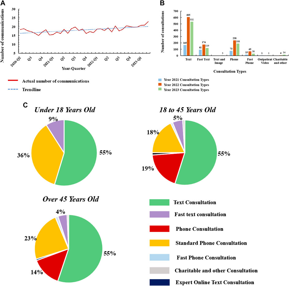
FIGURE 1. Good doctor online platform online consultation data (A), Quarterly consultation frequency data on the Good Doctor Online platform from 2020 to 2023. (B), Statistical analysis of consultation methods used by patients on the Good Doctor Online platform from 2020 to 2023. (C), Age distribution of patients consulting via the Good Doctor Online platform and the corresponding consultation methods.

3.2 The model

This network comprises a hierarchical, two-tiered network model that captures the geography, structure, and relationships within the Good Doctor website Health Community’s hospital distribution. Figure 2 is the structural framework of the network. This network model is constructed with three distinct nodes: hospital, city location, and province location, each representing different levels within the healthcare system’s geography. In this two-tiered network model, the first layer contains geographical locations of hospitals. The second layer further consider the number and weights of hospitals within a city or district, providing insight into the local healthcare infrastructure.

FIGURE 2

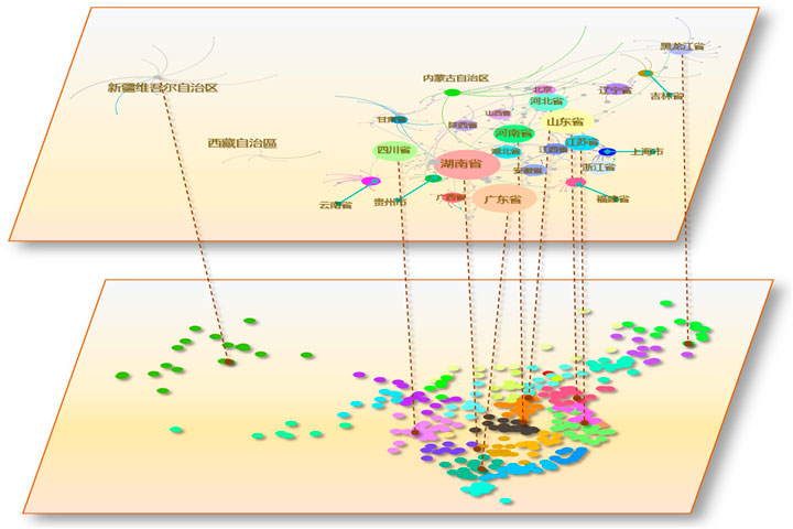
FIGURE 2. Structural framework of the two-tiered network model.

Table 1 show the tiered classification system for hospitals, as mandated by the administrative health departments of China, it provide a robust framework for assigning weights to nodes within the healthcare network. This system evaluates medical institutions across a three-tiered hierarchy, with each tier being further subdivided into ‘A' and ‘B' sublevels, signifying the institution’s caliber. Tier ‘3A’ representing the highest qualification achievable by mainland Chinese hospitals, they are predominantly located in major urban centers such as municipalities, provincial capitals, and large cities [29]. In accordance with the tiered classification system for hospitals, this study assigns distinct weights to various hospital tiers. The study use of these official tiers as nodes weights in the network analysis aptly reflects the role and significance of each hospital within the overarching healthcare delivery system.

TABLE 1

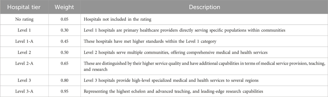
TABLE 1. Weight assignments for hospital tiers.

In the network’s architectural framework, each hospital is represented as a node, assigned a weight $W_h\left(i\right)$ that reflects its tier rating. This weight allocation is determined by a function $f$ based on Table 1 hospital tier. For the weighting of city location nodes, denoted as $W_{cl}$, the formula is structured as shown in Eq. 2:

$W_{cl}={\sum }_{i\in c}{W}_h\left(i\right)(2)$

the $W_{cl}$ of a city location node is the sum of the weights of all hospitals within the same location. $i\in C$ indicates all hospitals located within city $C$ .This hierarchical network edges include from hospital nodes to their respective location nodes, and edges between hospitals within the same Location.

In the second layer of our network model, we capture the broader regional and interurban dynamics by mapping the geographical affiliations between cities and provinces. In this layer, nodes representing provinces stand at the apex of the hierarchy, aggregating the data from subordinate city or district nodes. The formula is as follows (3):

$W_p={\sum }_{j\in p}{W}_{cl}\left(j\right)(3)$

where $W_p$ represents the weight of the province node. $i\in P$ indicates each city location node $j$ that falls within province $P$. $W_{cl}\left(j\right)$ is the weight of the city location node $j$, as defined in the first layer of the network. This hierarchical structure in the network allows for a comprehensive representation of the healthcare system’s physical and organizational structure. It incorporates the geographical affiliations and administrative boundaries of the provinces and their subordinate cities or districts. Notably, in this network model, all edges are considered unweighted, focusing solely on the relationships and connections among nodes.

4 Network analysis

4.1 Network visualization and characteristics analysis

Figure 3 exhibits the two-tiered network structural distribution, highlighting the China 34 provinces and cities and their significant nodes. Table 2 delineates the entire network characteristics, providing a comprehensive view of the network’s topology. The network, consisting of 10,365 nodes connected by 219,871 edges, exhibits an average degree of 42.426.

FIGURE 3

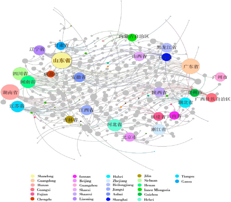
FIGURE 3. Structural distribution of the entire network.

TABLE 2

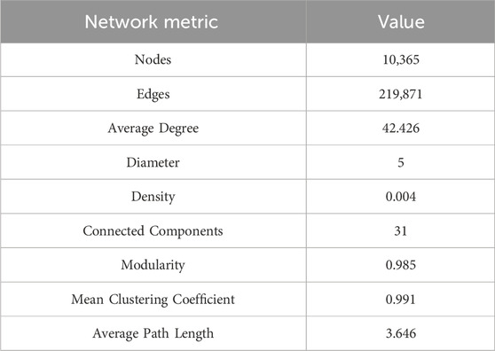
TABLE 2. Characteristics of the entire network.

This high average degree underlines a densely interconnected network, suggesting significant interaction and resource exchange among hospitals. The network maintains a diameter of 5, implying that the most distantly positioned nodes in the network can be connected via a relatively short path. This describes the rapid information transfer and coordination among hospitals, even though the distant geographical distance. The network density is 0.004, with many potential connections remaining unestablished. The structure features 31 connected components, and a high modularity score of 0.985. This modularity reflects the network’s organizational structure, mirroring administrative and geographical boundaries within the healthcare system. The mean clustering coefficient of 0.991 reflects a strong tendency for nodes to cluster together, indicating a tight-knit network with a high potential for collaboration and resource pooling among closely connected hospitals. The average path length 3.646 illustrates that the close connection of healthcare organizations. These topology characteristics point to the potential fractal nature of the network.

4.2 Scale-free and small-world properties analysis

4.2.1 Entire network analysis

Table 3 shows the entire network scale-free and small-world properties analysis result, and Figure 4 shows the entire network power-law fit of the degree distribution. Scale-free networks display a power-law degree distribution where few nodes serve as significant hubs, whereas small-world networks are characterized by short path lengths and high clustering, exemplifying the ‘six degrees of separation’ phenomena. This study examines these attributes through key metrics exploration of the network’s scale-free and small-world properties, including the Power-law Exponent (Table 3, Formula 6), Standard Error of the Power-law Exponent, Log-normal Mean (Table 3, Formula 7) and Standard Deviation (Table 3, Formula 8), Likelihood Ratio, and p-value. The Power-law Exponent highlights the network’s hub-centric nature, demonstrating a few nodes with extensive connections. Simultaneously, the Standard Error of this exponent offers a measure of estimation accuracy, enhancing the credibility of findings. To further dissect the network’s degree distribution, we employ the Log-normal Mean and Standard Deviation, providing insights into the central tendency and variability of connections on a logarithmic scale. The likelihood ratio and p-value are then compared to the fit of different distribution models, confirming the statistical robustness of our analysis. A power-law degree distribution is described by the formula [30]:

$P\left(k\right)\approx \mathrm{C}{k^{-}}^{\alpha }(4)$

where $P\left(k\right)$ denotes the probability of encountering a node with a degree $k$ within the network. $\mathrm{C}$ serves as a normalization constant to ensure that the total of the probability distribution sums to unity. $\alpha$ known as the power-law exponent, reflecting the structural heterogeneity of the network. $k$ symbolizes the degree of a node, signifying the count of its connections. This study employed Maximum Likelihood Estimation (MLE) for determining the power-law exponent ($\alpha$) [31]. MLE effectively aligns the power-law exponent with observed data, thereby capturing the scale-free nature of the network. The likelihood function for the power-law model is given by [32]:

$L\left(r;k\right)={\displaystyle \prod _{i=1}^n}p\left(k_i|\alpha \right)(5)$

TABLE 3

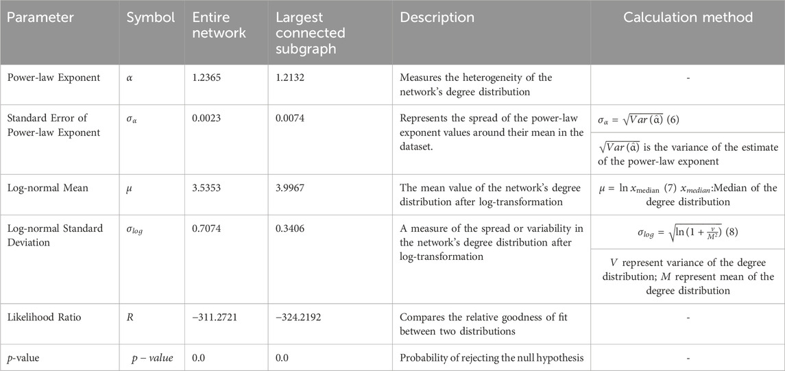
TABLE 3. Scale-free and small-world properties.

FIGURE 4

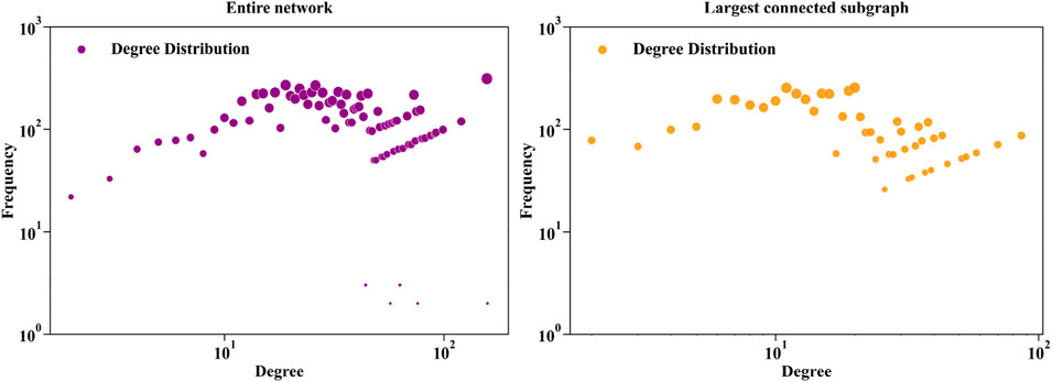
FIGURE 4. Power-law degree distribution in the entire network and largest connected subgraph.

The maximum likelihood function $L\left(\alpha ;k\right)$ is employed to estimate the optimal power-law exponent $\alpha$ in a given dataset. The exponent $\alpha$ is a key parameter in network analysis, reflecting how node connections are distributed and identifying whether the network exhibits scale-free characteristics and self-similarity. The degree $k_i$ of the $i^{th}$ node represents the number of connections it has, while $p\left(k_i|\alpha \right)$ denotes the probability of the $i^{th}$ node having a degree $k_i$ under the power-law distribution.

The power-law exponent $\alpha =1.2365$, although lower than the usual range of 2-3, highlights a notable feature of the network: a significant number of connections are concentrated among a small group of nodes. This suggests the presence of key ‘hub’ nodes within the network. The high average degree of 42.426 corroborates this, indicating that these hub nodes are extensively interconnected. This finding aligns with existing research on networks such as the Ythan Estuary and Silwood Park [33, 34]. The Standard Error of Power-law Exponent $\sigma =0.0023$, emphasizes the precision and reliability of the power-law exponent estimation. Log-normal Mean $\mu =3.5353$ and Standard Deviation ${\sigma }_{\mathit{log}}=0.7074$ indicate the central tendency and variability of the degree distribution on a logarithmic scale. The dispersion highlights the presence of both highly connected hubs and numerous lower-degree nodes, characteristic of scale-free networks. The negative Likelihood Ratio $R=-311.2721$ and the significant $p-value=0.0$ collectively suggest that the power-law distribution aptly models the network’s degree distribution, further supporting its scale-free nature.

4.2.2 Largest connected subgraph analysis

Figure 4 shows largest connected subgraph network power-law fit of degree distribution. Tables 3–5 show the network structure and various parameters of the largest connected subgraph (Shandong Province). These results show the largest connected subgraph network characteristics and parameter results of small-world and scale-free characteristics. The largest connected subgraph comprises 820 nodes and 12,976 edges. This indicates a substantial network size, signifying extensive healthcare connectivity within the province. Average Degree (28.202) demonstrates that each node in the network is directly connected to around 28 other nodes. It reflects a high level of direct interconnectivity among the nodes, indicative of a densely knit network. The small diameter (4) suggests small-world properties that the longest path between any two nodes in the network is relatively short. The network’s density (0.034), while indicative of a sparse overall structure, shows a reasonable level of connectivity given the network’s size. While not all possible connections are present, the existing ones form a coherent network. The high modularity (0.908) reflects a strong community structure within the network. This can imply a network division into sub-networks with dense internal connections. The Mean Clustering Coefficient (0.499) shows a moderate tendency of nodes to cluster together. It indicates the presence of localized groups or communities within the network. The short average path length (1.267) signals efficient information or resource transfer across the network, essential for quick response and coordination in healthcare services.

TABLE 4

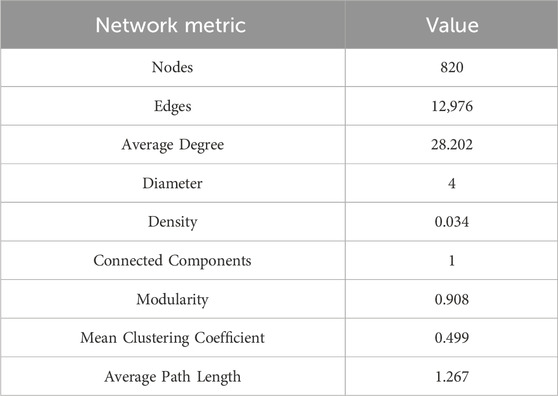
TABLE 4. Network characteristics of the largest connected subgraph.

TABLE 5

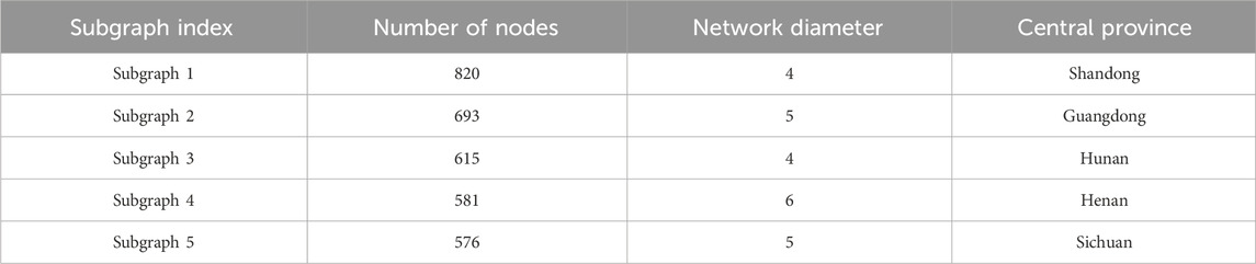
TABLE 5. Connectivity and diameter metrics of network subgraphs.

In further network feature analysis, the power-law exponent $\alpha =1.2132$ (1.2132) indicates a certain level of inhomogeneity in the network’s connectivity, with some nodes having significantly more connections than others. Standard Error of Power-law Exponent $\sigma =0.0074$ lending credibility to the scale-free nature of the network. Log-normal Mean $\mu =3.9967$ and Standard Deviation ${\sigma }_{\mathit{log}}=0.3406$ are indicates a degree distribution with a broad range of node connectivity. The log-normal mean of 3.9967 reflects that the central tendency of node connections, when transformed to a logarithmic scale, leans towards a higher value. This suggests that while there are nodes with an extensive number of connections, a significant portion of the network comprises nodes with relatively fewer connections. The standard deviation of 0.3406, being a measure of spread on the log scale, shows that the degree distribution has some variability but not extremely wide-ranging. The negative Likelihood Ratio $R=-324.2192$ and the significant $p-value=0.0$ , these statistics support the suitability of the log-normal distribution for modeling the network’s degree distribution, suggesting that the degree distribution follows a log-normal pattern more closely than a power-law. Given these observations, the Largest connected subgraph exhibits properties conducive to fractal analysis.

As illustrated in Table 5 and Figure 5, in this model the provinces such as Shandong, Guangdong, Hunan, Henan, and Sichuan have substantial medical network sizes. As reflected by the number of network connectivity results, highlighting their significance within the national medical network. Notably, Shandong Province, with the largest connected subgraph, demonstrates it provides essential services to the Large base population. Given the requirements for network connectivity and representativeness in subsequent research, the largest connected subgraphs were chosen as the basis for fractal analysis. This choice is grounded not only on the consideration of node quantity but also on the importance of this subgraphs within the overall network structure.

FIGURE 5

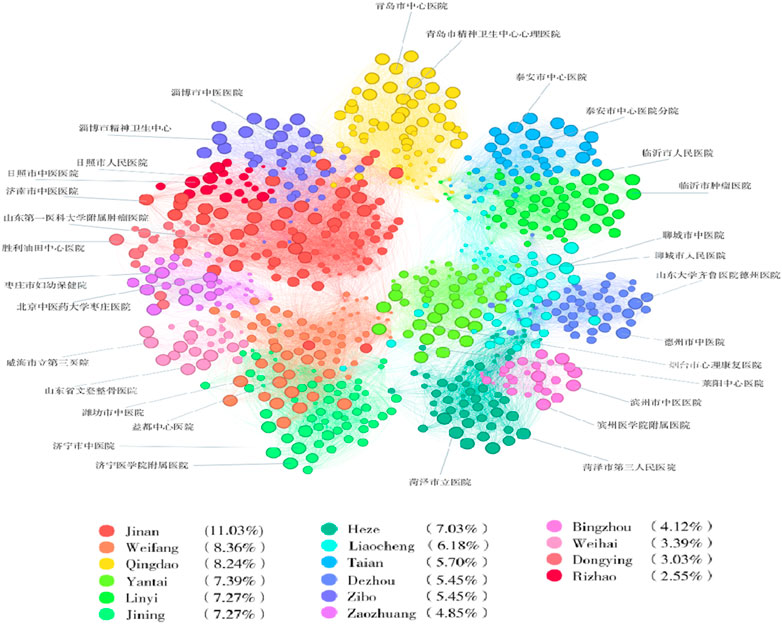
FIGURE 5. Structural network of the largest connected subgraph (shandong province).

4.2.3 Largest connected subgraph assortativity coefficient analysis

To gain a deeper understanding of the network’s connectivity patterns and their self-similar characteristics across different scales, we further computed the assortativity coefficient of the largest connected subgraph. It is calculated by comparing the degree distribution of nodes in the network to the degree distribution of their neighbors. The formula for calculating the assortative coefficient, as shown in 9, is as follows [35]:

$r=\frac{\frac{1}{E}{\sum }_i{j}_i{k}_i-{\left[\frac{1}{2E}{\sum }_i\left(j_i+k_i\right)\right]}^2}{\frac{1}{2E}{\sum }_i\left(j_i^2-k_i^2\right)-{\left[\frac{1}{2E}{\sum }_i\left(j_i+k_i\right)\right]}^2}(9)$

Here, $E$ represents the total number of edges, $j_i$ and $k_i$ are the degrees of the nodes at either end of edge $i$. The assortative coefficient r ranges from $-1$ to $+1$, where $+1$ indicates perfect assortative mixing, $-1$ indicates perfect disassortative mixing, and 0 indicates no assortative, implying random connections between nodes. In this study, the calculated result revealed a high positive assortative, the assortativity coefficient of the network is $r=0.998$. This suggests that nodes of high degree tend to connect with other high-degree nodes, while low-degree nodes tend to connect with other low-degree nodes. Such a pronounced pattern of assortative may indicate a strong community structure within the network, an important marker of fractal properties, suggesting consistency in connectivity patterns across different scales.

Furthermore, the power-law distribution analysis for the entire network and the largest connected subgraphs has highlighted the presence of hub nodes within the network. These nodes possess unusually high connections, serving as central pivots around the network. Such a structural configuration suggests that similar connectivity patterns may be observed across different scales, indicating the potential fractal nature of the network.

5 Experimental results

5.1 Calculation of fractal dimension

In the quest to quantify the fractal dimension of the Good Doctor website Health Community’s hospital distribution network, the Compact Box Burning (CBB) [36] algorithm offers a viable approach. However, the inherent randomness in the node selection process for box occupation within the CBB algorithm can inadvertently disrupt the structural integrity of the network. This is particularly problematic in geographical or social network, where nodes exhibit complex dependency relations, necessitating a higher number of boxes to achieve comprehensive network coverage [37]. Such randomness can decrease the accuracy of node coverage within boxes and fail to preserve network connectivity. To address the limitations of the CBB method, this study employs a centrality-based box-counting approach to calculate the fractal dimension of the network structure [37, 38]. The methodology unfolds as follows:

Define the box size $l_b$, and construct a set $\mathit{C}$ containing all uncovered nodes.

Select the node $i$ with the highest centrality and include all nodes within a shortest path distance $l_i<l_b$ as part of the box.

Count the number of boxes $N_b\left(l_b\right)$ required to cover the entire network at box size $l_b$.

Repeat steps 2 and 3 until the set $\mathit{C}$ is empty, culminating in the calculation of the fractal dimension $d_b$ as a characteristic feature of the network’s fractal structure. The fractal dimension is estimated as follows (10) [22]:

$d_b=\frac{\ln N_b\left(l_b\right)}{\ln \left(l_b\right)}(10)$

Here, $d_b$ represents the fractal dimension of box $b$, $l_b$ is the size of the box, and $N_b\left(l_b\right)$ is the minimum number of boxes of size $l_b$ required to cover the entire network. Furthermore, to accurately quantify the network’s fractal dimension, our study employed a linear regression analysis on the outcomes of the centrality-based box-counting method. By analyzing the logarithmic relationship between box sizes and the count of boxes required for coverage, we determined the network’s fractal dimension. This centrality-based methodology not only mitigates the issue of structural integrity loss but also enhances the precision of network coverage, thus providing a more accurate representation of the network’s fractal nature.

5.2 Renormalization group analysis

This study employed the hospital node weights (0.05, 0.5, 0.65, 0.8) as varied thresholds network and calculated fractal dimensions. Networks $G_{wn}$ at each threshold were defined by removing edges with weights below the specified value $w_n$. To preserve the network’s structural integrity and connectivity, we concentrated our analysis on the largest connected subgraph. In this study, we concentrated on three primary parameters for fractal analysis: Fractal Dimension, Regression Coefficient, and Regression Intercept. The Fractal Dimension serves as a metric to characterize fractal patterns or sets, quantifying complexity as the ratio of change in detail relative to scale change. Typically, a fractal dimension approaching or exceeding 2 indicates a network structure of high complexity and interconnectivity [22]. The Regression Coefficient reveals the network’s complexity variation across different scales, determined through logarithmic transformations of box sizes and counts. A coefficient near −1 suggests a proportional relationship between these log-transformed values, while significant deviations from −1 indicate a more intricate relationship, highlighting the scale-dependent nature of the network’s complexity. Meanwhile, the Regression Intercept provides an initial complexity measure at the smallest scale analyzed, with higher values generally pointing to increased complexity at these smaller scales. Applying renormalization group analysis to this subgraph across the range of threshold weights unveiled distinct power-law decays.

Figure 6 and Table 6 present the network’s fractal dimension and regression analysis. These findings underscore that at a threshold weight of 0.5, the network’s fractal characteristics are most pronounced. At threshold 0.05 ($w_n=0.05$): The fractal dimension is 0.426, indicating relatively low structural complexity when including the weakest connections. The regression coefficient of −0.426 suggests a straightforward relationship between box size and count after logarithmic transformation, with network complexity not significantly varying across scales. A higher regression intercept of 5.694 indicates a certain level of structural complexity even at the smallest scale, suggesting that even weak connections play a role in the network structure at smaller scales.

FIGURE 6

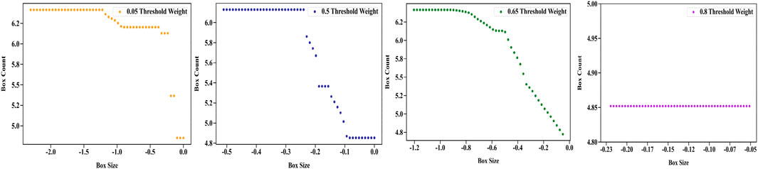
FIGURE 6. Fractal dimension analysis at multiple thresholds.

TABLE 6

TABLE 6. Fractal dimension and regression analysis results at multiple thresholds.

Elevating the threshold to 0.50 ($w_n=0.5$): The fractal dimension increases significantly to 3.197, demonstrating pronounced fractal properties and dense connectivity when considering Level 2 hospitals after excluding lower-weight nodes. The regression coefficient of −3.197 indicates a significant increase in network complexity with scale. The regression intercept of 4.865, lower than that at 0.05 threshold, suggests that although overall complexity is high, complexity at the smallest scale is relatively lower.

At threshold 0.65 ($w_n=0.65$): The fractal dimension stands at 2.211, maintaining relatively high structural complexity while considering higher-tier (Level 2A–3A) hospitals. The regression coefficient of −2.211 reflects significant but less pronounced changes in network complexity across scales compared to the threshold to 0.50 ($w_n=0.5$). The regression intercept at 4.612 indicates further reduced complexity at the smallest scale, showing that as the threshold increases, the network tends toward a more simplified structure.

At threshold 0.80 ($w_n=0.80$): The fractal dimension reduces to 0.345, suggesting the loss of most fractal characteristics and a shift towards a more simplified and centralized structure when focusing on the highest-tier (Level 3-3A) hospitals. The regression coefficient of −0.345 implies a simpler relationship between complexity and scale changes, predominantly influenced by strong connections among top-tier hospitals. The regression intercept of 4.815, slightly higher than at the 0.65 threshold, indicates a tendency towards a more centralized network structure at the highest threshold.

The fractal analysis of the network, particularly at the threshold weight of 0.5, unveils a pronounced fractal nature, marking it as a pivotal point for capturing the network’s structural dynamics. Here, the network demonstrates a dense and interconnected fabric. This complexity signifies a resilient system, particularly evident when considering secondary (Level 2) hospitals. As the threshold weight increases beyond this point, there is a noticeable shift in the network’s fractal characteristics. This transition is marked by a decrease in fractal properties, leading to a more centralized and simplified structure, suggesting that the network’s intricacy is most optimally represented at the mid-level threshold.

5.3 Self-similarity and assortativity coefficient analysis

This research conducts an in-depth analysis of secondary and higher-level network hospitals in Shandong Province, emphasizing the shifts in power-law exponents across three specific threshold values: 0.5, 0.65, and 0.8. In the field of network science, self-similarity refers to the characteristic of a network in maintaining similar structural features across various scales. A pivotal metric for assessing self-similarity in networks is the power-law exponent. This exponent quantifies the distribution of node degrees, offering a measure of how connections within the network are dispersed among nodes. The calculation of the power exponent is the same as the MLE method, using formulas (4) and (5).

Table 7 delineates the power-law exponent analysis for both the original network and its largest connected component (LCC) at varying thresholds by the aforementioned method. Figure 7 presents the degree distributions of the network under varying thresholds. At the $w_n=0.5$ threshold, which aligns with Level 2 hospitals, the original network exhibits a power-law exponent of $\alpha =1.225$, whereas the LCC demonstrates a slightly lower exponent of $\alpha =1.073$. This indicates a substantial presence of highly connected nodes within the network. As the threshold increases to $w_n=0.65$, aligning with Level 2-A hospitals, the exponent for the original network slightly decreases to $\alpha =1.180$, and the LCC to $\alpha =1.054$. This shift suggests a marginal decrease in network density, yet connectivity remains notably concentrated. Elevating the threshold to $w_n=0.8$, which includes only Level 3 hospitals, leads to a significant reduction in the original network’s power-law exponent, dropping to $\alpha =0.964$, while the LCC is at $\alpha =1.036$. Original network’s power-law exponent substantial decline reflects the scarcity of higher-tier hospitals in the network, resulting in a sparser network structure. Despite variations in thresholds, the LCC consistently maintains a higher power-law exponent.

TABLE 7

TABLE 7. Power law exponent analysis at multiplet thresholds.

FIGURE 7

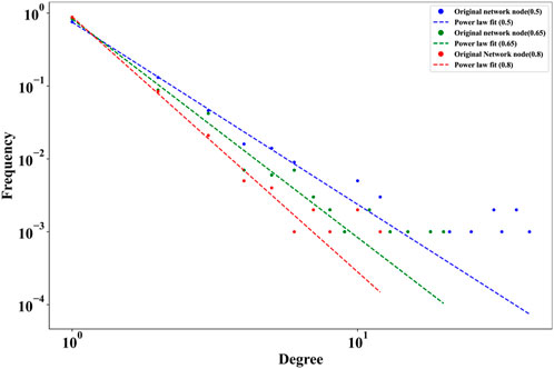
FIGURE 7. Degree distribution and power law fit at multiple thresholds.

Table 8 shows the assortativity coefficient analysis for different threshold weights, revealing the network’s connectivity patterns among various hospital tiers. At the 0.5 Threshold, the assortativity coefficient $r=0.971$ indicates a highly assortative network structure. This high correlation underscores a homophilous connectivity pattern within the network. At 0.65 Threshold, there is a slight decrease in the assortativity coefficient $r=0.945$. This reduction signals a gradual diversification in the network’s connectivity. Level 2-A and higher-tier hospitals have started to establish more connections with different-tier hospitals but are primarily still maintaining network assortativity. At the 0.8 Threshold, the assortativity coefficient further decreases $r=0.865$. This marked decline reflects an increased heterogeneity in the network’s structure. Top-tier hospitals (Level 3-3A) demonstrate a tendency to form connections with a wider variety of hospital tiers, leading to a more diversified.

TABLE 8

TABLE 8. Assortativity coefficient analysis at multiple thresholds.

This result demonstrates that the network distribution of secondary hospitals exhibits self-similarity and assortativity characteristics at different thresholds. Additionally, the largest connected component (LCC) of the network at different thresholds shows smaller change in power-law exponent values, thereby maintaining a degree of structural consistency.

6 Discussion and conclusion

This study provides valuable insights into the fractal nature and power-law characteristics of Chinese hospital network. The importance of secondary hospitals is emphasized in ensuring equitable distribution and improving the accessibility to healthcare resources. Allocating additional resources to these essential healthcare centers, particularly secondary hospitals, is expected to elevate public access to medical services. This enhancement is crucial for meeting immediate healthcare needs and ensuring the long-term stability and robustness of the healthcare network. The necessity of a balanced, strategically dispersed healthcare network is underscored. Optimizing resource allocation and service delivery across different healthcare levels is imperative for a resilient, responsive, and fair healthcare system.

Of course, certain limitations and future directions should be acknowledged. One of the primary constraints of this research is the scope of data, which, although comprehensive, is limited to a static in time. Healthcare networks are dynamic, with patterns of connectivity and hospital roles evolving in response to policy changes, technological advances, and public health needs. For future work, it is considered to design a multi-faceted analytical approach that incorporates economic development indices, political support for healthcare, and administrative efficiency across different provinces. Further research could also benefit from tracking changes to observe the effects of healthcare reforms and investments. Such a study could help improve the resilience of the healthcare system.

Secondly, the analyze method is limited to network characteristics analysis. The introduce of machine learning models may help uncovered hidden patterns under the network, informing future healthcare policy decisions.

Lastly, collaboration with urban planners and public health experts could yield a comprehensive framework that aligns hospital network development with broader urbanization objectives. This inter-disciplinary approach could facilitate a more holistic view of healthcare provision, where network analysis informs both the strategic placement of new hospitals and the optimization of existing resources.

Data availability statement

The original contributions presented in the study are included in the article/supplementary material, further inquiries can be directed to the corresponding authors.

Author contributions

HG: Conceptualization, Funding acquisition, Investigation, Writing–original draft. Y-FC: Data curation, Resources, Visualization, Writing–original draft. KS: Formal Analysis, Visualization, Writing–review and editing. T-FZ: Methodology, Project administration, Supervision, Writing–review and editing.

Funding

The author(s) declare financial support was received for the research, authorship, and/or publication of this article. This work was supported by the Fundamental Research Funds for Central Universities under Grant No. 23JNQN50. HG and Y-FC finished the data collection and analysis and finish the drift manuscript. KS and T-FZ provided technique support and revised the paper.

Conflict of interest

The authors declare that the research was conducted in the absence of any commercial or financial relationships that could be construed as a potential conflict of interest.

Publisher’s note

All claims expressed in this article are solely those of the authors and do not necessarily represent those of their affiliated organizations, or those of the publisher, the editors and the reviewers. Any product that may be evaluated in this article, or claim that may be made by its manufacturer, is not guaranteed or endorsed by the publisher.

References

1. Kwon BC, Kim S-H, Lee S, Choo J, Huh J, Yi JS. VisOHC: designing visual analytics for online health communities. IEEE Trans Vis Comput Graph (2015) 22(1):71–80. doi:10.1109/tvcg.2015.2467555

PubMed Abstract | CrossRef Full Text | Google Scholar

2. De Boer MJ, Versteegen GJ, Van Wijhe M. Patients’ use of the Internet for pain-related medical information. Patient Educ Couns (2007) 68(1):86–97. doi:10.1016/j.pec.2007.05.012

PubMed Abstract | CrossRef Full Text | Google Scholar

3. Zhang X, Liu S, Deng Z, Chen X. Knowledge sharing motivations in online health communities: a comparative study of health professionals and normal users. Comput Hum Behav. (2017) 75:797–810. doi:10.1016/j.chb.2017.06.028

CrossRef Full Text | Google Scholar

4. Lu C, Zhang Z, Lan X. Impact of China’s referral reform on the equity and spatial accessibility of healthcare resources: a case study of Beijing. Soc Sci Med (2019) 235:112386. doi:10.1016/j.socscimed.2019.112386

PubMed Abstract | CrossRef Full Text | Google Scholar

5. Penchansky R, Thomas JW. The concept of access: definition and relationship to consumer satisfaction. Med Care (1981) 19:127–40. doi:10.1097/00005650-198102000-00001

PubMed Abstract | CrossRef Full Text | Google Scholar

6. Soja EW. Seeking spatial justice. Minneapolis, MN, USA: U of Minnesota Press (2013).

Google Scholar

7. Wang F. Why public health needs GIS: a methodological overview. Ann GIS (2020) 26 (1):1–12. doi:10.1080/19475683.2019.1702099

PubMed Abstract | CrossRef Full Text | Google Scholar

8. Rosero-Bixby L. Spatial access to health care in Costa Rica and its equity: a GIS-based study. Soc Sci Med (2004) 58(7):1271–84. doi:10.1016/s0277-9536(03)00322-8

PubMed Abstract | CrossRef Full Text | Google Scholar

9. Salze P, Banos A, Oppert JM, Charreire H, Casey R, Simon C, et al. Estimating spatial accessibility to facilities on the regional scale: an extended commuting-based interaction potential model. Int J Health Geogr (2011) 10:2–16. doi:10.1186/1476-072x-10-2

PubMed Abstract | CrossRef Full Text | Google Scholar

10. Delamater PL. Spatial accessibility in suboptimally configured health care systems: a modified two-step floating catchment area (M2SFCA) metric. Health Place (2013) 24:30–43. doi:10.1016/j.healthplace.2013.07.012

PubMed Abstract | CrossRef Full Text | Google Scholar

11. Luo W, Wang F. Measures of spatial accessibility to health care in a GIS environment: synthesis and a case study in the Chicago region. Environ Plan B Plan Des (2003) 30(6):865–84. doi:10.1068/b29120

CrossRef Full Text | Google Scholar

12. Hao H. The development of online doctor reviews in China: an analysis of the largest online doctor review website in China. J Med Internet Res (2015) 17(6):e134. doi:10.2196/jmir.4365

PubMed Abstract | CrossRef Full Text | Google Scholar

13. Mandelbrot B. How long is the coast of Britain? Statistical self-similarity and fractional dimension. Science (80-. ) (1967) 156(3775):636–8. doi:10.1126/science.156.3775.636

PubMed Abstract | CrossRef Full Text | Google Scholar

14. Kinsner W. A unified approach to fractal dimensions. Int J Cogn Inform Nat. Intell. (2007) 1(4):26–46. doi:10.4018/jcini.2007100103

CrossRef Full Text | Google Scholar

15. Aguirre J, Viana RL, Sanjuán MAF. Fractal structures in nonlinear dynamics. Rev Mod Phys (2009) 81(1):333–86. doi:10.1103/revmodphys.81.333

CrossRef Full Text | Google Scholar

16. Hart JC. Fractal image compression and recurrent iterated function systems. IEEE Comput Graph Appl (1996) 16(4):25–33. doi:10.1109/38.511849

CrossRef Full Text | Google Scholar

17. Song C, Havlin S, Makse HA. Origins of fractality in the growth of complex networks. Nat Phys (2006) 2(4):275–81. doi:10.1038/nphys266

CrossRef Full Text | Google Scholar

18. Gallos LK, Song C, Havlin S, Makse HA. Scaling theory of transport in complex biological networks. Proc Natl Acad Sci (2007) 104(19):7746–51. doi:10.1073/pnas.0700250104

PubMed Abstract | CrossRef Full Text | Google Scholar

19. Rozenfeld HD, Song C, Makse HA. Small-world to fractal transition in complex networks: a renormalization group approach. Phys Rev Lett (2010) 104(2):025701. doi:10.1103/physrevlett.104.025701

PubMed Abstract | CrossRef Full Text | Google Scholar

20. Thung F, Bissyande TF, Lo D, Jiang L. Network structure of social coding in github. In: 2013 17th European conference on software maintenance and reengineering; March, 2013; Genova, Italy. IEEE (2013). p. 323–6.

CrossRef Full Text | Google Scholar

21. Kim JS, Goh K-I, Kahng B, Kim D. A box-covering algorithm for fractal scaling in scale-free networks. Chaos Interdiscip J Nonlinear Sci (2007) 17(2):026116. doi:10.1063/1.2737827

PubMed Abstract | CrossRef Full Text | Google Scholar

22. Song C, Gallos LK, Havlin S, Makse HA. How to calculate the fractal dimension of a complex network: the box covering algorithm. J Stat Mech Theor Exp. (2007) 2007(03):P03006. doi:10.1088/1742-5468/2007/03/p03006

CrossRef Full Text | Google Scholar

23. Song C, Havlin S, Makse HA. Self-similarity of complex networks. Nature (2005) 433(7024):392–5. doi:10.1038/nature03248

PubMed Abstract | CrossRef Full Text | Google Scholar

24. Zhou W-X, Jiang Z-Q, Sornette D. Exploring self-similarity of complex cellular networks: the edge-covering method with simulated annealing and log-periodic sampling. Phys A Stat Mech Its Appl (2007) 375(2):741–52. doi:10.1016/j.physa.2006.10.025

CrossRef Full Text | Google Scholar

25. Sturmberg JP, O’Halloran DM, Martin CM. Understanding health system reform–a complex adaptive systems perspective. J Eval Clin Pract (2012) 18(1):202–8. doi:10.1111/j.1365-2753.2011.01792.x

PubMed Abstract | CrossRef Full Text | Google Scholar

26. Karperien AL, Jelinek HF. Fractal, multifractal, and lacunarity analysis of microglia in tissue engineering. Front Bioeng Biotechnol (2015) 3:51. doi:10.3389/fbioe.2015.00051

PubMed Abstract | CrossRef Full Text | Google Scholar

27. Natalia YA, Faes C, Neyens T, Chys P, Hammami N, Molenberghs G. Fractal dimension based geographical clustering of COVID-19 time series data. Sci Rep (2023) 13(1):4322. doi:10.1038/s41598-023-30948-7

PubMed Abstract | CrossRef Full Text | Google Scholar

28. Neutens T, Schwanen T, Witlox F, De Maeyer P. Equity of urban service delivery: a comparison of different accessibility measures. Environ Plan A (2010) 42(7):1613–35. doi:10.1068/a4230

CrossRef Full Text | Google Scholar

29. Zheng W, Sun H, Zhang P, Zhou G, Jin Q, Lu X. A four-stage DEA-based efficiency evaluation of public hospitals in China after the implementation of new medical reforms. PLoS One (2018) 13(10). doi:10.1371/journal.pone.0203780

PubMed Abstract | CrossRef Full Text | Google Scholar

30. Muchnik L, Pei S, Parra LC, Reis SDS, Andrade Jr JS, Havlin S, et al. Origins of power-law degree distribution in the heterogeneity of human activity in social networks. Sci Rep (2013) 3(1):1783. doi:10.1038/srep01783

PubMed Abstract | CrossRef Full Text | Google Scholar

31. Myung IJ. Tutorial on maximum likelihood estimation. J Math Psychol (2003) 47(1):90–100. doi:10.1016/s0022-2496(02)00028-7

CrossRef Full Text | Google Scholar

32. Jeske DR. On maximum-likelihood estimation of clock offset. IEEE Trans Commun (2005) 53(1):53–4. doi:10.1109/tcomm.2004.840668

CrossRef Full Text | Google Scholar

33. Albert R, Barabási A-L. Statistical mechanics of complex networks. Rev Mod Phys (2002) 74(1):47–97. doi:10.1103/revmodphys.74.47

CrossRef Full Text | Google Scholar

34. Garlaschelli D, Caldarelli G, Pietronero L. Universal scaling relations in food webs. Nature (2003) 423(6936):165–8. doi:10.1038/nature01604

PubMed Abstract | CrossRef Full Text | Google Scholar

35. Newman MEJ. Assortative mixing in networks. Phys Rev Lett (2002) 89(20):208701. doi:10.1103/physrevlett.89.208701

PubMed Abstract | CrossRef Full Text | Google Scholar

36. Song Y-Q, Liu J-L, Yu Z-G, Li B-G. Multifractal analysis of weighted networks by a modified sandbox algorithm. Sci Rep (2015) 5(1):17628. doi:10.1038/srep17628

PubMed Abstract | CrossRef Full Text | Google Scholar

37. Zhang H, Lan T, Li Z. Fractal evolution of urban street networks in form and structure: a case study of Hong Kong. Int J Geogr Inf Sci (2022) 36(6):1100–18. doi:10.1080/13658816.2021.1974451

CrossRef Full Text | Google Scholar

38. Molinero C, Murcio R, Arcaute E. The angular nature of road networks. Sci Rep (2017) 7(1):4312. doi:10.1038/s41598-017-04477-z

PubMed Abstract | CrossRef Full Text | Google Scholar