 Yong Guo
- School of Electronic and Information Engineering, Anshun University, Anshun, China
Introduction: In this study, the spatial bending vibration of macro- and/or micro-scale cantilevered fluid-conveying pipes is investigated through finite dimensional analysis.
Methods: Firstly, the Galerkin method is employed to discretize the partial differential equations of motion of the system into a system of ordinary differential equations. Then, the projection method based on center manifold-normal form theory is adopted to derive the coefficient formula that determines the pipe’s nonlinear dynamic behaviors, i.e., the change rate of the real part of the critical eigenvalue with respect to the flow velocity and the nonlinear resonance term, thereby obtaining reduced-order equations. Compared to previous studies that relied on the numerical solution of ordinary differential equations to determine the existence and stability of periodic motion, this paper concludes the existence and stability of periodic motion by utilizing the coefficients of the Galerkin discretized equations and the reduced-order equations, significantly saving time in determining the dynamic properties of pipes.
Results and discussion: Subsequently, by investigating the reduced-order equations under specific parameters, the existence and stability of the two types of periodic motion of the pipe are studied. For macro pipes, the truncated mode numbers are set incrementally to calculate the coefficients of the reduced-order equations, investigate the distribution of the stability of the two types of periodic motions with the mass ratio, and carry out a longitudinal comparison (i.e., the comparison between the results obtained under different truncated mode numbers) as well as a horizontal comparison (i.e., the comparison of results between the finite dimensional analysis and the infinite dimensional analysis). It is found that the reasonable truncated mode number required to study this type of system is 15. Previous studies primarily focused on the convergence of frequency and amplitude when determining the truncated mode numbers. On this basis, our study further examines the convergence of motion forms with respect to the truncated mode numbers. Finally, based on the Galerkin discretization equations of 15 modes, the distribution of the stability of two types of the periodic motion of micro pipes with the mass ratio is analyzed. For macro- and micro-scale pipes, when the truncated mode number is 15, the error between the finite dimensional analysis results and the infinite dimensional analysis results is calculated to be about 7%. The above results are verified by obtaining the numerical solution to Galerkin discretization equations.
1 Introduction
Fluid-conveying pipe is an important engineering structure, and its dynamic behaviors have been extensively and deeply studied. Early studies mainly focused on the establishment of motion equations and the linear vibration of pipelines [1–5]. Holmes was the first to investigate the nonlinear vibration of fluid-conveying pipes [6, 7]; in this literature, the processing method based on Galerkin discretization was called “finite dimensional analysis” [6], and the processing method based on function space projection was called “infinite dimensional analysis” [8]. The terms “finite dimensional analysis” and “infinite dimensional analysis” used in our study are derived from the definition given by Holmes. Rousselet and Herrmann [9] used the Krylov-Bogoliubov method to investigate the coupled nonlinear vibration of the cantilevered fluid-conveying pipe and the fluid in the pipes and analyze the variation law of the periodic motion amplitude of the pipe with the mass ratio. Based on the n-mode (n = 1, 2, or 3) discrete system of the motion equation of fluid-conveying pipes, Namchchivaya and Tien [10], Jayaraman and Narayaman [11], and Namchchivaya [12] studied the nonlinear parametric vibration of simply supported pipes at both ends; Chang and Chen [13], Li and Paidoussis [14] investigated the nonlinear parametric vibration of cantilevered pipes. Paidoussis et al. [15] considered the cantilevered fluid-conveying pipe subject to motion constraints; these motion constraints were simplified to a cubic nonlinear spring, which is the source of the nonlinear term of the system. In their study, the chaotic motion of the pipe was studied by the 2-mode Galerkin discretization of the original motion equation. Based on [15], Paidoussis and Semler [16] added the geometric nonlinearity caused by a large amplitude and used 2, 3, and 4 modes to discretize the original vibration equation; it was found that 2-mode Galerkin discretization equations can produce qualitatively accurate results, and 4-mode Galerkin discretization equations can produce quantitatively accurate results. Based on [15], Jin [17] added linear spring constraints and analyzed the influence of linear spring stiffness on the chaotic motion of the system by using 2-mode Galerkin discretization equations. Paidoussis and Semler [18] considered the nonlinear vibration of a cantilevered fluid-conveying pipe with an intermediate support spring, where the “nonlinear term” originating from the geometric nonlinearity was due to a large amplitude motion. In their study, based on 2-mode Galerkin discretization equations, various bifurcation phenomena of the system were investigated with the center manifold-normal form theory. Paidoussis and Semler [19] presented a general process of using the center manifold-normal form method to study the dynamic behavior of cantilevered fluid-conveying pipes, and numerical calculations were conducted by using Galerkin discretization equations of 2, 3, and 4 modes respectively. Subsequently, Paidoussis and Semler [19] found that the impact of truncation mode numbers on the calculation results was not obvious, and it was considered the essential dynamic characteristics of the system can be only extracted with low-order discretization equations. Until 2006, in the literature using the Galerkin method to investigate fluid-conveying pipes, the number of truncation modes generally did not exceed 4 [20–23]. It worths mentioning that the above-mentioned references are all studies on two-dimensional (2D) motions of fluid-conveying pipes.
Since the study by Wadham-Gagnon et al. [24], great attention was paid to the dynamics of three-dimensional (3D) vibrations of cantilevered fluid-conveying pipes. Following the modified Hamilton principle [1], Wadham-Gagnon et al. [24] derived a new 3D version of nonlinear governing equations for cantilevered fluid-conveying pipes by incorporating an additional mass at the free end of the pipe and springs support. Note that this equation is consistent with the equation derived by Lundgren et al. [25] using the force balance method when factors such as terminal mass and intermediate spring support are not considered. Based on this new 3D model, Modarres-Sadeghi et al. [26] investigated the motion switches of cantilevered fluid-conveying pipes between 2D and 3D with increasing flow velocity, where 8-mode Galerkin discretization equations were used at most. Additionally, the 3D motion of cantilevered fluid-conveying pipes with additional intermediate springs support [27], with an end mass [28], or with both an end mass and springs support [29] was been studied. In Ref. [27], using 4-mode Galerkin discretization equations, Païdoussis et al. conducted a theoretical and experimental study of 3D nonlinear dynamics of cantilevered pipes with external springs, involving five different cases in terms of attachment, spring configurations, and stiffnesses. Results indicated that the system may lose stability either via flutter or divergence, depending on the specific case of spring support. Compared to Ref. [27], a more complete (chaotic motion and far more extensive experimental investigation), accurate (a larger number of Galerkin’s truncation modes, where 8-mode Galerkin discretization equations were used at most), and interesting (richer dynamical behaviors) work was completed by Ghayesh and Païdoussis [30]. In Refs. [28, 29], to achieve the convergence of calculation, up to 10-mode Galerkin discretization equations were used. For pipes with a large end-mass, the resulting dynamics becomes much richer than that of pipes without any external attachments. Furthermore, it was found that for a very large end-mass, many Galerkin’s truncation modes (where 12-mode Galerkin discretization equations were used at most) are required to obtain convergent results [31]. By introducing a lateral base excitation, Chang and Modarres-Sadeghi [32] extended the equations proposed by Wadham-Gagnon et al. [24] and applied them to investigate the possibility of controlling the pipe’s 3D motion and/or limiting it to a 2D motion in a pre-defined direction by changing the base excitation frequency and amplitude, where 8-mode Galerkin discretization equations were used at most.
Due to the recent technological development in engineering practice, the characteristic size of structures become smaller and smaller [33–36], including the micro beam [37–39] with Winkler elastic foundation [40], micro torus plate [41], micro cylindrical shell [42, 43], micro-structure on elastic foundation [44], and fluid-conveying micro pipe [45]. The study of micro-scale pipes is an important research direction of the dynamics of fluid-conveying pipes. Yang et al. [46] discussed the geometric nonlinearity caused by axial stretching and investigated the free vibration of micropipes based on the modified couple stress theory (MCST), where the number of truncation modes was 1. Dai et al. [47] studied the buckling and post-buckling vibrations of carbon nanotubes (CNTs), calculated the buckling configuration of the tube when the fluid velocity in the pipe exceeded a critical value using a theoretical method, and derived a differential equation for the vibration of the pipe under this configuration. The post-buckling vibration of the pipe was studied by using the Galerkin method, and the number of truncation modes was 2. Bahaadini and Hosseini [48] examined the fluid-conveying CNTs in a magnetic field and investigated the buckling and vibration of the tube under different boundary conditions, where the number of truncation modes was 8. Bahaadini and Hosseini [49] studied the effect of dissipation on the stability of viscoelastic CNTs and comprehensively determined the viscosity coefficient and microscale effect on the system frequency and critical flow velocity, where the number of truncation modes was 8. Hu et al. [50] considered micro-scale cantilevered fluid-conveying pipes subject to motion constraints that were simplified into a smoothed-trilinear cubic model, where based on 4-mode Galerkin discretization equations, the impact of micro-scale effects and motion constraints on the dynamic behavior of the pipe was studied. It was found that the micro-scale parameters can make the pipe more stable, and the motion constraints make the system exhibit richer dynamic phenomena. Dai et al. [51] established a completely nonlinear vibration equation of cantilever fluid-conveying pipes under the action of electrostatic force, in which the nonlinear term was included by a nonlinear electrostatic force and geometric nonlinearity caused by a large amplitude. Based on Galerkin discretization equations of 4 modes, the impact of voltage on the stability boundary of the pipe was investigated. Ghayesh et al. [52] investigated the parametric vibration of CNTs fixed at both ends. By analyzing Galerkin discretization equations of 8 modes, it was found that the average flow velocity and amplitude of the fluid in the pipe significantly affect the path of the pipe to chaotic vibration. Zhu et al. [53] investigated the impact of viscoelastic foundation and partially distributed tangential force on the dynamics of cantilever CNTs, where the number of truncation modes was 8. In the comprehensive study by Sarparast et al. [54], the effects of various parameters, including magnetic flow, scale parameters, flow velocity, axial spin speed, Y-shaped downstream elbow angle, concentrated masses, attached springs, surface effects, and complex environments on the vibration characteristics of the cantilevered pipe and pinned-pinned pipe were analyzed, where the number of truncation modes was 7.
For the dynamics of fluid-conveying pipes, some studies do not perform Galerkin discretization on partial differential equations but directly use other methods. By using the perturbation method for analysis, Bajaj et al. investigated the Hopf bifurcation of planar cantilevered fluid-conveying pipes [55] and parametric vibration [56] and studied the type and stability of the periodic motion of symmetrical and asymmetric spatial cantilevered fluid-conveying pipes [57, 58] and spatial parametric vibration [59]. Yamashita et al. considered the interaction between the second-order and third-order modes of a cantilevered fluid-conveying pipe with a concentrated mass [60] and a spring constrained [61] attached to its free end under planar vibration. At this time, the complex frequencies corresponding to the second- and third-order modes had positive real parts, and these two modes were excited to perform interactions. Yamashita et al. [62] considered the spatial vibration of a cantilevered fluid-conveying pipe with a concentrated mass attached to the free end and investigated the “in-plane and out-of-plane” interactions of its second- and third-order modes based on the results reported in Ref. [60]. The methods used in references [60–62] were all projection methods [63], and the coefficients of the reduced-order equations were all determined by numerical calculations. Zhang and Huang [64] adopted a mode analysis method to study the effect of Poisson, junction, and friction couplings on the stability of cantilevered fluid-conveying pipes. Amiri et al. [65] studied the planar linear vibration of a micro-scale cantilevered fluid-conveying pipe in a spring-damper environment and subjected to temperature and magnetic loads. They used the extended Galerkin method (i.e., mode analysis method) to analyze the critical flow velocity and flutter frequency of the pipe by considering the boundary value problem of the differential equation. In references [66, 67] by Jin and Ren, the post-buckling equilibrium configuration was obtained by the two-step perturbation technique, and it was used as the initial configuration to establish a differential equation of perturbation motion for forced vibration analysis and parametric resonance study of FG nanotubes, where the effects of the flow velocity, material gradient, and different scales on the nonlinear dynamic behaviors were discussed. In another paper by Jin et al. [68], the analogous method was applied to obtain the amplitude-frequency response curves for pulsatile fluid-conveying FG nanopipes with movable boundary. The static deformation and flutter for cantilevered fluid-conveying curved pipes were studied experimentally by Chehreghani et al. [69]. Guo et al. applied the center manifold-normal form method to study the symmetric bifurcation [70] and asymmetric bifurcation [71] of the micro-scale cantilevered fluid-conveying pipe. The differential quadrature method was also widely used in the vibration research of fluid-conveying pipes [72, 73]. Incidentally, other methods applied to investigate the dynamics of structures, e.g., the Navier discretization method [74], eigenvalue and eigenvector method [75–77], successive approximation method [78], Fourier series method [79], compact analytical method [80], may also be suitable for the analysis of fluid-conveying pipe’s dynamics.
The literature review above indicates that most studies on the dynamics of fluid-conveying pipes adopt the Galerkin method. However, there is no unified conclusion on how many truncation modes should be taken. Among the majority of literatures, the truncated mode numbers generally do not exceed 8. Although some literature has conducted convergence analysis based on frequency or amplitude, the corresponding motion form of the same frequency or amplitude may also be different, i.e., it may be planar motion or spatial motion. Thus, it is necessary to examine the convergence of motion with respect to the number of truncation modes. Meanwhile, the mass ratio has an important impact on the dynamic characteristics of fluid-conveying pipes. However, most of the existing studies using the Galerkin method investigate the convergence of the calculation results at one or a few specific mass ratios. The number of truncation modes obtained in this way cannot be extended to a wide range of mass ratios. In view of this, in almost the entire mass ratio interval, by investigating the change law of the “distribution of periodic motion stability along the mass ratio” with the number of truncation modes and combined with infinite dimensional analysis results, this study summarizes the reasonable truncation mode numbers required when investigating the dynamics of macro- and/or micro-cantilevered fluid-conveying pipes with the Galerkin method, thus making the truncation modes applicable to a wide range of mass ratios while ensuring the convergence of motion forms.
The rest of this paper is organized as follows. In Section 2, the 3D bending vibration equation of a macro- and/or micro-cantilevered fluid-conveying pipe with O (2) symmetry is given based on previous studies. In Section 3, by using the Galerkin technique, the original vibration equation is discretized into a set of ordinary differential equations. Then, by utilizing the projection method based on the center manifold and normal form theory, the discretized systems are reduced to a two-degree-of-freedom nonlinear ordinary differential equation. It is worth mentioning that previous studies mainly relied on the numerical resolutions of Galerkin discretized equations for pipe. However, when the numbers of mode truncation are considerable, the numerical resolutions of these ordinary differential equations become exceedingly time-consuming. If the periodic motion patterns of the pipe can be determined based on the coefficients of the discretized equations, it would expedite the determination of the dynamic properties of pipes. The reduced-order equations proposed here precisely fulfill this research requirement. In Section 4, the truncation mode numbers are taken incrementally for a macro pipe. The convergence of the linear term coefficients of the reduced-order equations is analyzed, and the stability of the periodic motion determined by the nonlinear term coefficients of the reduced-order equations is investigated. By comparing the results given by different truncation mode numbers and the results of infinite dimensional analysis, the reasonable truncation mode numbers needed to study this type of system are summarized and applied to the study of micro-scale pipes. The reasonable numbers of mode truncation summarized through the aforementioned process ensures the convergence of frequency, amplitude, and motion forms. For macro- and/or micro-cantilevered fluid-conveying pipes, the errors between the finite dimensional analysis results and the infinite dimensional analysis results are calculated. Finally, some conclusions are drawn in Section 5.
2 Mechanics models and differential equations of motion
The motions equations [70] are derived on the basis of the following assumptions [24, 81]:
(1) the fluid is incompressible;
(2) the fluid is plug-flow and the flow velocity is constant;
(3) the pipe is modelled as a nonlinear Euler-Bernoulli beam;
(4) the transverse deflections of the pipe could be large, but the strains in the pipe are small;
(5) rotatory inertia and shear deformation are neglected;
(6) the centroid line of the pipe is inextensible;
(7) for micro-scale pipe, the pipe is made of materials of which size-dependent behaviors can be predicted by the MCST [82].
As shown in Figure 1A, the macro- and micro-scale cantilevered fluid-conveying pipe with a length of
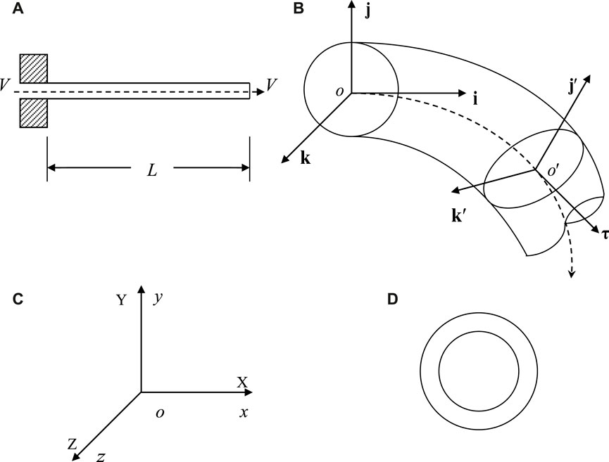
Figure 1. (A) The schematic of the macro- and micro-scale cantilevered fluid-conveying pipe; (B) 3D flexural vibration; (C) Coordinate systems; (D) The circular cross-section of the macro- and micro-scale pipe.
As shown in Figure 1C, when the pipe is not deformed, the straight line where the pipe centerline is located is the
In the following, a curvilinear coordinate
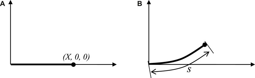
Figure 2. The centroid line of the pipe is not stretchable: (A) before the deformation; (B) after the deformation.
At moment t, it is assumed that the position of one point on the centerline of the pipe
where
For the vibration of a slender pipe, the Euler-Bernoulli beam model can be adopted. The resulting dimensionless form of the motions equations and boundary conditions is shown below [70]:
where
are all dimensionless quantities. In Eq. 6, G is the Lamé’s constant and l is a material length scale parameter date from MCST [82], which has been used to analyze various micro-structures [84–86]. The dimensionless parameter
3 Galerkin discretization and reduced-order equations
3.1 Galerkin discreted equations
Given that the mode functions of the cantilever beam satisfy boundary condition (5), they can be selected as basis functions [2, 16, 17, 90]. According Galerkin method, let the solutions to Eqs. 4a and 4b be
where
where
and
Transform Eq. 9 into a first-order form:
In Eq. 12
where
where
3.2 Reduced-order equations
3.2.1 Critical flow velocity
By examining the degeneracy of the linear part of Eq. 12, the critical flow velocity can be given.
Eq. 17 can be written as
where “
In Eq. 18, “
It can be seen that
Considering
3.2.2 Reduced-order equations
At a given
Denote
The high-dimensional (specifically, 4n-dimensional, where n is the number of truncation modes) ordinary differential system (12) can be reduced and simplified to a 4-dimensional equations according to the method described in [70] (
where
Both
The coefficients
where
considering the form of
where
According to Eqs 15, 16, the following results can be obtained.
These Eqs 28 and 29 are the specific forms of Eq. 26, where
In this way, Eq. 26, i.e., the specific form of
3.2.3 Periodic motion and its stability
For Eq. 23, by taking polar coordinate transformation
Only when
With this scale transformation, Eq. 30 becomes
Then, variable substitution
where
and
In Eq. 32,
Thus one can write Eq. 35 in the following form
where (·) denotes the derivative with respect to slow time ετ and
The equilibrium points of the averaging Eq. 36 correspond to the periodic motions of the original Eq. 23, and the stability of the two equations corresponds to each other in the case of nondegeneracy.
Regardless of whether
4 The influences of mode truncation number and “reasonable mode truncation numbers”
This study considers the nonlinear dynamic characteristics of the macro pipe (
4.1 Case of macro-pipes (
4.1.1 Influence of the mode truncation number on the critical flow velocity-mass ratio curve and the critical frequency-mass ratio curve
The critical flow velocity-mass ratio curves and the critical frequency-mass ratio curves obtained by different orders of Galerkin truncation are different. The curves are drawn for the mode truncation numbers of n = 2, n = 4, n = 6, n = 8, n = 9, n = 11, n = 13, and n = 15. Then, the curves are compared with the exact solution reported in Ref. [70].
As shown in Figure 3A, C, the critical flow velocity-mass ratio curves and the critical frequency-mass ratio curves obtained by the Galerkin method are almost consistent with the exact solution when the mode truncation number is 8 and 9. Meanwhile, Figure 3B and Figure 3D shows that the critical flow velocity-mass ratio curves and the critical frequency-mass ratio curves given by the Galerkin method show almost no change when the mode truncation number increases from 8. Thus, for the prediction of critical flow velocity and critical frequency, the Galerkin truncation using 8 modes can obtain quite accurate results. Then, when the actual flow velocity exceeds the critical flow velocity, what type of motion will occur for the pipe conveying fluid, and can the Galerkin discretization of the 8 modes accurately predict its dynamic characteristics? These issues are analyzed below. The analysis result indicates that, in the prediction of the dynamic behavior of the fluid-conveying pipe after instability occurs, the Galerkin discretization of 8 modes cannot provide accurate results, and more modes truncations are required for accurate predictions.
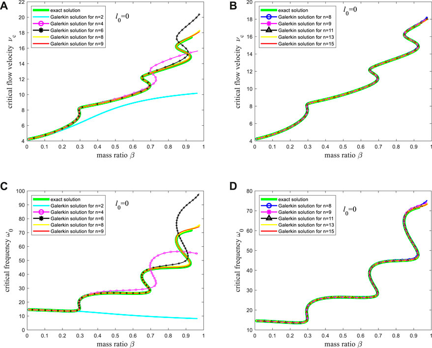
Figure 3. The critical flow velocity-mass ratio curve: (A) The exact solution and the solutions corresponding to the mode truncation numbers 2, 4, 6, 8, and 9; (B) The exact solution and the solutions corresponding to the mode truncation numbers 8, 9, 11, 13, and 15; The critical frequency-mass ratio curve: (C) The exact solution and the solutions corresponding to the mode truncation numbers 2, 4, 6, 8, and 9; (D) The exact solution and the solutions corresponding to the mode truncation numbers 8, 9, 11, 13, and 15.
4.1.2 Influences of the mode truncation number on periodic motion
Based on the above analysis, the following figures show the data (Eqs 24 and 25) required for the reduced-order Eq. 23 and the data [
(a) The change rate of the real part of the critical eigenvalue under different mode truncation numbers, i.e.,
From Figure 4A, it can be seen that the change rate of the real part of the critical eigenvalue provided by the Galerkin method is highly consistent with the exact solution when the mode truncation number is 8 and 9. A more detailed comparison, as shown in Figure 4B, indicates that the exact solution of the change rate of the real part of the critical eigenvalue is completely consistent with the Galerkin solution when the mode truncation number is 9, 11, 13, and 15, respectively. In contrast, compared with the other solutions in Figure 4B, when the mode truncation number is 8, the Galerkin solution has a little deviation in the tail (i.e., the section where the mass ratio is greater than 0.9). Hence, for predicting the change rate of the real part of the critical eigenvalue, the Galerkin truncation of 9 modes can already obtain quite accurate results. The research in [70] indicates that (i) at
(b) The nonlinear resonance term (see Eqs 37, 25) and the stability criterion of periodic motion (
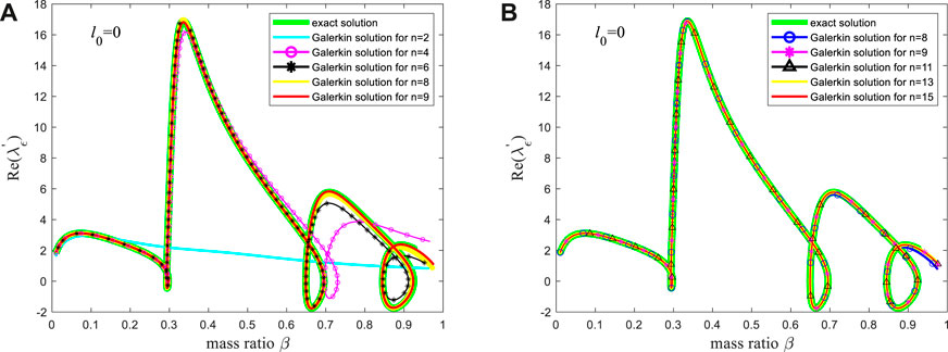
Figure 4. The rate of change of the real part of the critical eigenvalue: (A) The exact solution and the solutions corresponding to the mode truncation numbers as 2, 4, 6, 8, and 9, respectively; (B) The exact solution and the solutions corresponding to the mode truncation numbers as 8, 9, 11, 13, and 15, respectively.
Based on the above analysis about the effect of the mode truncation number on the critical flow velocity-mass ratio curve, the critical frequency-mass ratio curve and the change rate of the real part of the critical eigenvalue, let us start with n = 9 and take the truncation mode numbers incrementally to obtain the reasonable truncated mode number required to study this type of system. Subsequently, the resolutions of the ordinary differential equations set (9) are conducted using Runge-Kutta methods.
When n = 9, Figures 5A–C shows the variation curve of the high-order term coefficient with the mass ratio, and Figures 5D, E demonstrates the stability of the two types of periodic motion. A mass ratio of β = 0.92 [represented by “o” in Figures 5D,E] and a flow velocity of
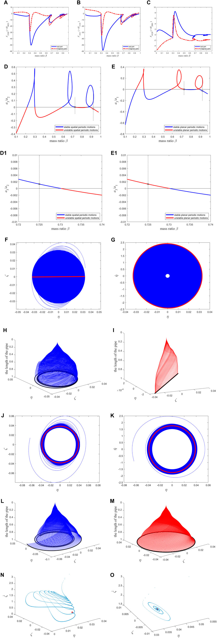
Figure 5. The resonance term coefficients of the second-order discretization equation of the macro pipe, the stability of two types of periodic motion, the phase diagram, and the configuration diagram: (A–C) The coefficients of the reduced-order equations; (D) the stability of spatial periodic motion; (E) the stability of planar periodic motion. (D1) and (E1) The enlarged version of (D, E) near the “*”. (F) the position relationship of the free ends of the pipe in two directions; (G) the velocity-displacement relationship diagram of the free ends of the pipe in one direction; (H) the transient process of the whole pipe vibration; (I) the steady-state vibration of the whole pipe. The blue (red) color represents the transient (steady-state) motion in (F–I). The interpretation of (J–M) is compared to (F–I); The Poincaré map: (N) corresponding to (F–I); (O) corresponding to (J–M). The blue points correspond to transient motion, and the red points correspond to steady-state motion (i.e., fixed point).
It needs to be explained that in the drawing of Figure 5H, I, the displacement of point
It is significant that the nonlinear terms have an important influence on the dynamics of pipe. For the same parameters as Figures 5F-G, if only linear terms considered, the displacement and velocity of pipe will go toward infinity, as shown in Figure 6.
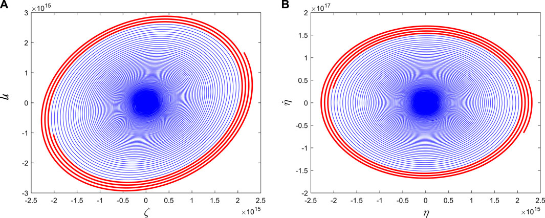
Figure 6. (A) The position relationship of the free ends of the pipe in two directions; (B) the velocity-displacement relationship diagram of the free ends of the pipe in one direction.
To compare with the results obtained when n = 11 in the following section, this study here sets the mass ratio β = 0.725 [represented by “*” in Figures 5D, E, and Figure 5(D1, E1) is the enlargement near the “*”] and the flow velocity
When n = 11, Figures 7A–C shows the variation curve of the high-order term coefficient with the mass ratio, and Figures 7D, E presents the stability of the two types of periodic motion.
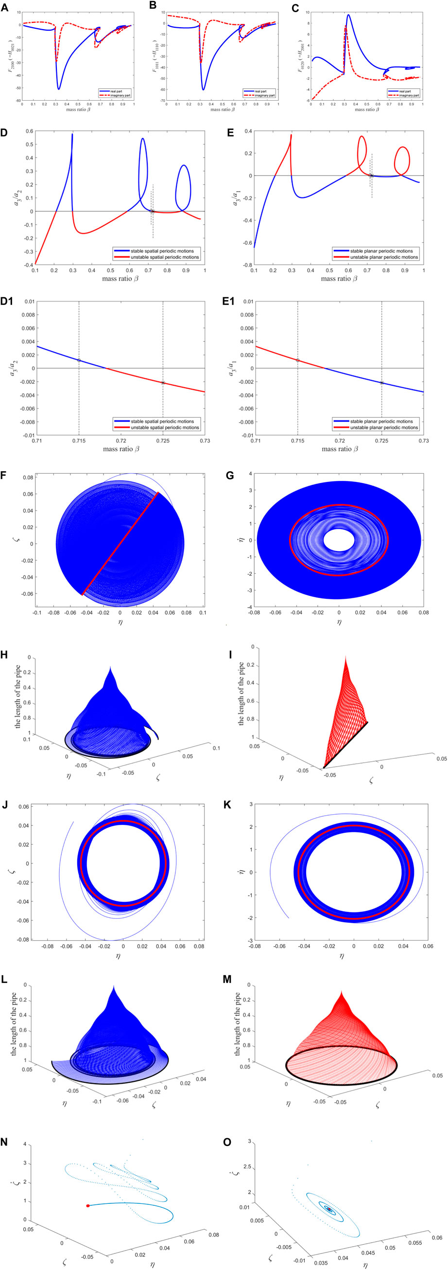
Figure 7. The resonance term coefficients of the second-order discretization equation of the macro pipe, the stability of two types of periodic motion, the phase diagram, and the configuration diagram: (A–C) The coefficients of the reduced-order equations; (D) the stability of spatial periodic motion; (E) the stability of planar periodic motion. (D1) and (E1) The enlarged version of (D) and (E) near the “*” and “o”. The interpretation of (F–I) is compared to Figures 5F–I. The interpretation of (j–m) is compared to Figures 5J–M; The Poincaré map: (N) corresponding to (F–I); (O) corresponding to (J–M). The blue points correspond to transient motion, and the red points correspond to steady-state motion (i.e., fixed point).
The results obtained when n = 11 have a minor correction to the results obtained when n = 9, as can be seen from the following comparison. This study sets a mass ratio of β = 0.725 again {represented by “*” in Figures 7D, E, and Figure 7(D1, E1) is the enlargement near the “*”} and a flow velocity of
To compare with the results obtained when n = 13 in the following section, this study here sets the mass ratio β = 0.715 [represented by “O” in Figures 7D, E, and Figure 7 (D1, E1) is the enlargement near the “O”] and the flow velocity
When n = 13, Figures 8A–C illustrates the variation curve of the high-order term coefficient with the mass ratio, and Figures 8D,E depicts the stability of the two types of periodic motion.
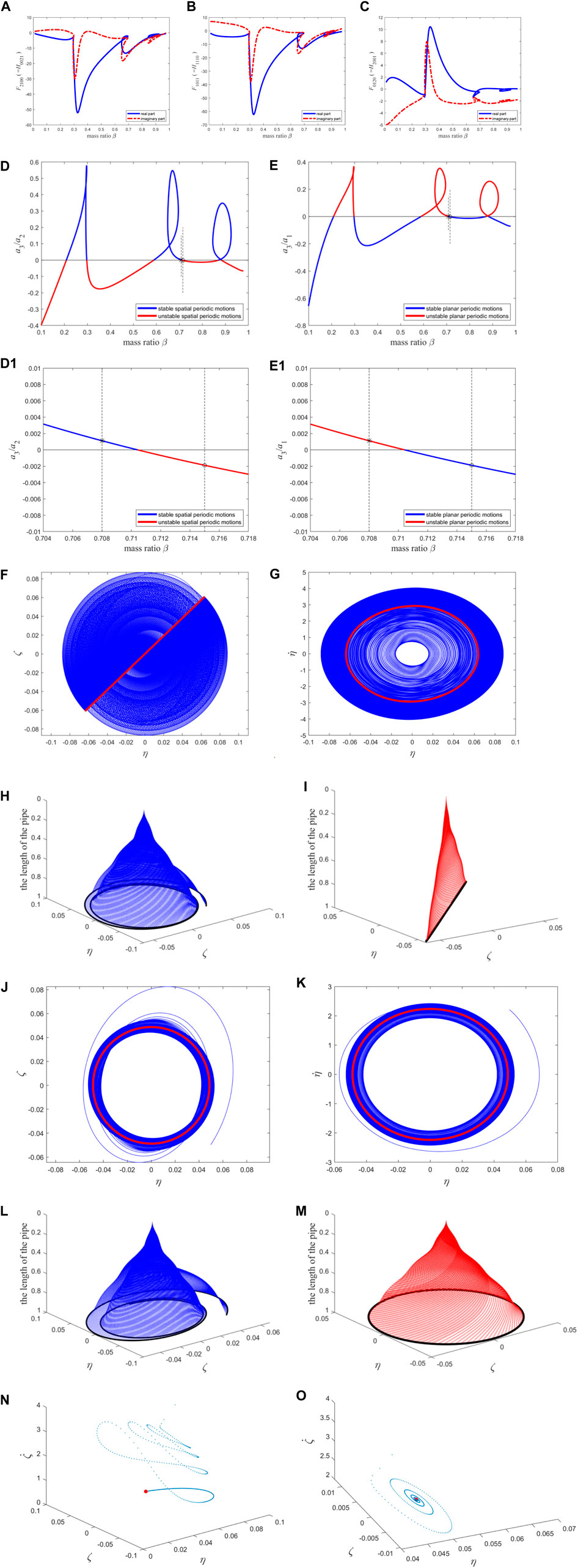
Figure 8. The resonance term coefficients of the second-order discretization equation of the macro pipe, the stability of two types of periodic motion, the phase diagram, and the configuration diagram: (A–C) The coefficients of the reduced-order equations; (D) the stability of spatial periodic motion; (E) the stability of planar periodic motion. (D1) and (E1) The enlarged version of (D) and (E) near the “*” and “o”. The interpretation of (F–I) is compared to Figures 5F–I. The interpretation of (J–M) is compared to Figures 5J–M; The Poincaré map: (N) corresponding to (F–I); (O) corresponding to (J–M). The blue points correspond to transient motion, and the red points correspond to steady-state motion (i.e., fixed point).
The results obtained when n = 13 have a minor correction to the results obtained when n = 11, as indicated by the comparison below. This study sets a mass ratio of β = 0.715 again [represented by “O” in Figures 8D,E, and Figures 8(D1, E1) is the enlargement near the “O”] and a flow velocity of
To compare with the results obtained when n = 15 in the following section, this study here sets the mass ratio β = 0.708 [represented by “*” in Figures 8D, E, and Figures 8(D1, E1) is the enlargement near the “*”] and the flow velocity
When n = 15, Figures 9A–C shows the variation curve of the high-order term coefficient with the mass ratio, and Figures 9D, E demonstrates the stability of the two types of periodic motion.
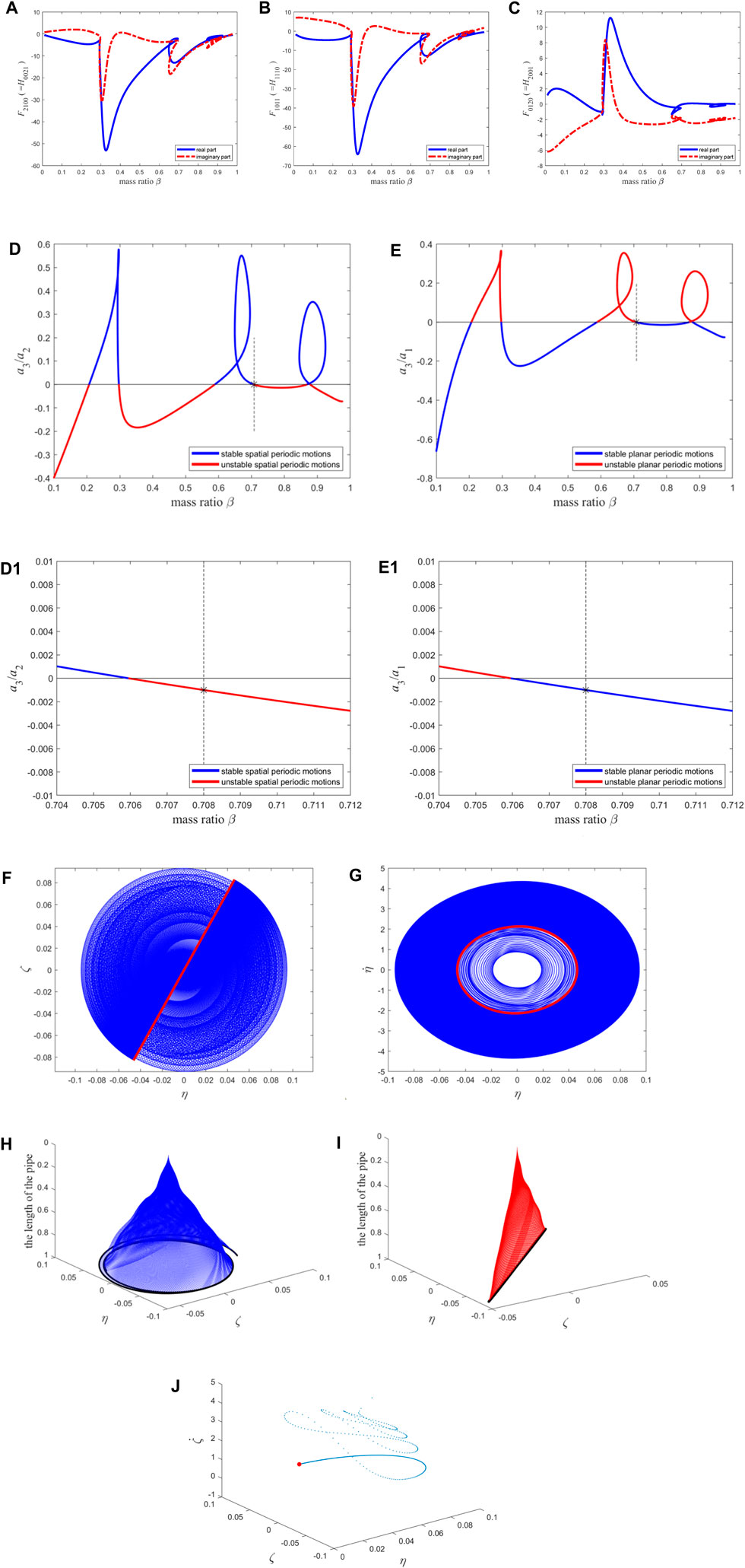
Figure 9. The resonance term coefficients of the second-order discretization equation of the macro pipe, the stability of two types of periodic motion, the phase diagram, and the configuration diagram: (A–C) The coefficients of the reduced-order equations; (D) the stability of spatial periodic motion; (E) the stability of planar periodic motion. (D1) and (E1) The enlarged version of (D) and (E) near the “*”. The interpretation of (F–I) is compared to Figures 5F–I; (J) The Poincaré map corresponding to (F–I). The blue points correspond to transient motion, and the red points correspond to steady-state motion (i.e., fixed point).
The results obtained when n = 15 have a minor correction to the results obtained when n = 13, as indicated by the following comparison. This study sets a mass ratio of β = 0.708 again [represented by “*” in Figures 9D, E, and Figures 9(D1, E1) is the enlargement near the “*”] and a flow velocity of
When n = 16, Figures 10A–C presents the variation curve of the high-order term coefficient with the mass ratio, and Figures 10D, E shows the stability of the two types of periodic motion.
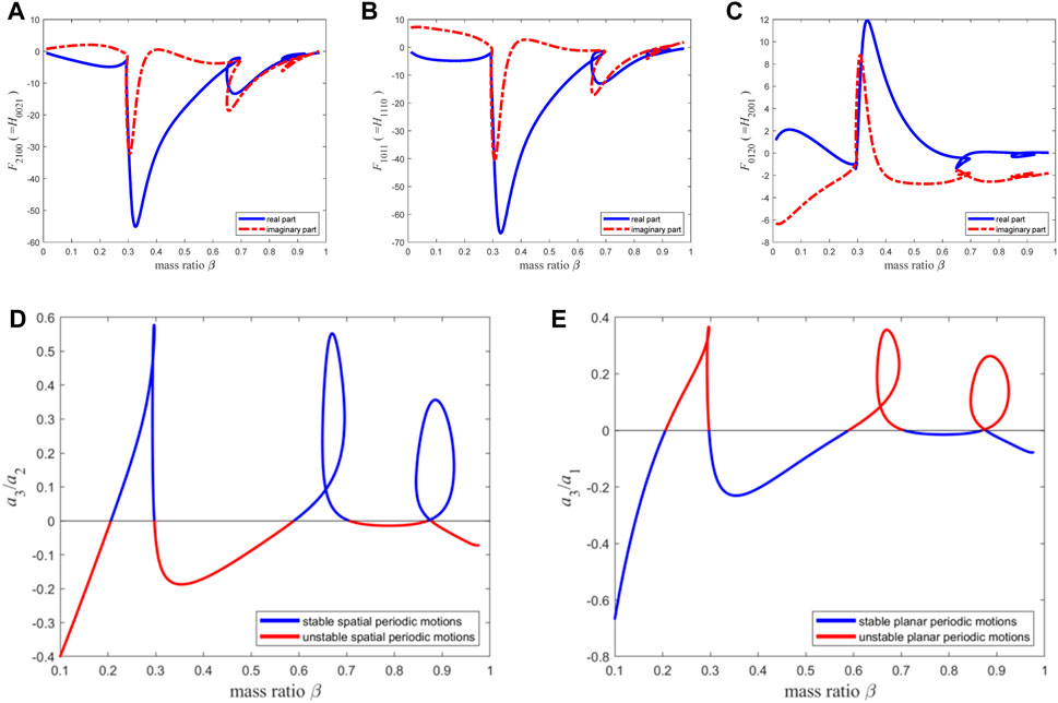
Figure 10. The resonance term coefficients of the second-order discretization equation of the macro pipe, the stability of two types of periodic motion: (A–C) The coefficients of the reduced-order equations; (D) the stability of spatial periodic motion; (E) the stability of planar periodic motion.
By comparing Figures 9D,E and Figures 10D, E, it is found that the two sets of figures are basically consistent in predicting the pipe’s periodic motion properties (as shown by Figure 11). Thus, when using the Galerkin method to investigate the qualitative dynamic behavior of this type of system, the reasonable mode truncation number should be set to 15, at which point the results have converged. Meanwhile, the results obtained at the mode truncation number of 15 are compared with those obtained based on infinite dimensional analysis in Ref. [70] (as shown in Figures 12A, B). It can be observed that in predicting the qualitative dynamic behavior of the system, the two sets of figures are also very close, and the difference lies in circles 1 to 5 and rectangles 1 to 5. Then, Figure 12(A1–A5) and Figure 12(B1–B5) are obtained by enlarging circles 1 to 5 and rectangles 1 to 5, respectively. The difference between the finite dimensional analysis results with the mode truncation number of 15 and that in Ref. [70] is represented by the black and magenta points in the figure. By calculating the distance between the black point and the magenta point in each figure in Figure 12(A1–A5), the sum of the distances is obtained as 0.0701. After conducting the same calculation for Figure 12(B1–B5), the sum of the distances is also 0.0701. Therefore, for this macro pipe, the error between the results of finite dimensional analysis and infinite dimensional analysis is only 7.01%, indicating a high level of coincidence. In the following section, for finite dimensional analysis of micro-scale pipes (
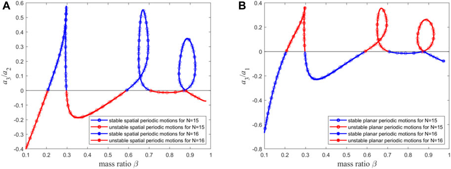
Figure 11. (A) The stability of spatial periodic motion for n = 15 and 16; (B) The stability of planar periodic motion for n = 15 and 16.
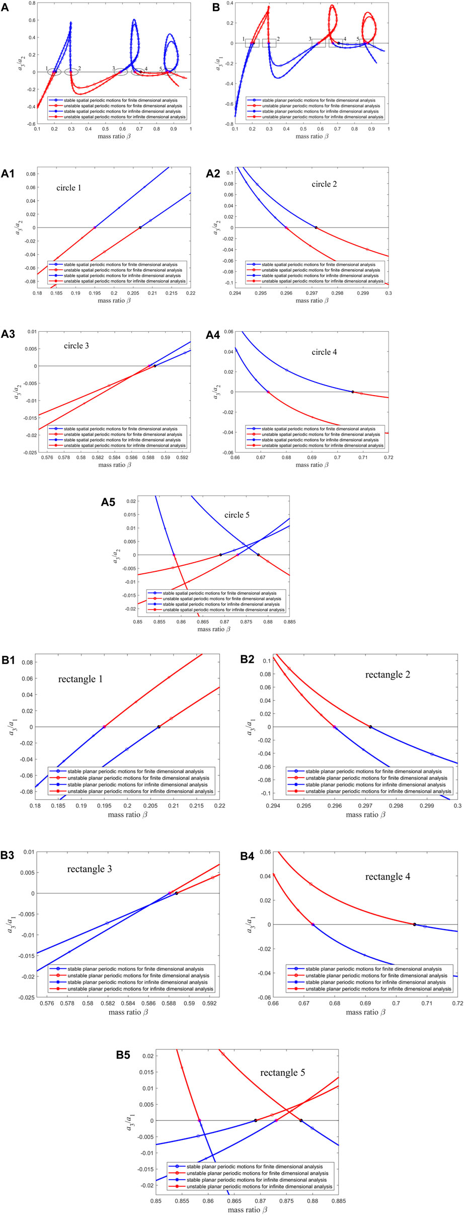
Figure 12. (A) The stability of spatial periodic motion for infinite dimensional analysis and finite dimensional analysis with n = 15; (B) The stability of planar periodic motion for infinite dimensional analysis and finite dimensional analysis with n = 15. (A1–A5) The enlarged version of circles 1 to 5 in (A); (B1–B5) The enlarged version of rectangles 1 to 5 in (B).
4.2 Case of micro-scale pipes (
The values of characteristic length l in Eq. 6 are dependent on the materials made of pipes, which are given by [93].
where μ is the Poisson’s ratio and
When the mode truncation number is set to 15, the critical flow velocity-mass ratio curves and the critical frequencies-mass ratio curves of the two types of micro-scale pipes are illustrated in Figures 13A,C, and the variation curve regarding the change rate of the real part of the critical eigenvalue [i.e.,
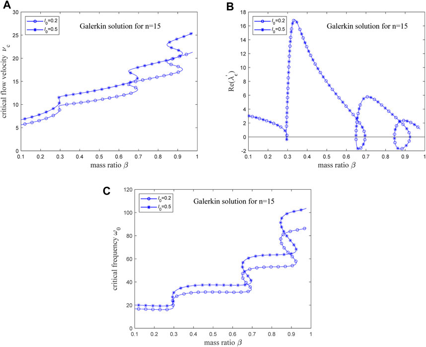
Figure 13. (A) The critical flow velocity-mass ratio curve for micro-scale pipes; (B) The rate of change of the real part of the critical eigenvalue for micro-scale pipes; (C) The critical frequencies-mass ratio curve for micro-scale pipes.
Reference [91] investigated the linear vibration characteristics of microscale cantilevered fluid-conveying pipes, in which the material and geometrical properties for micro-scale pipe constituents and fluid are taken as: l = 17.6 μm, E = 1.44 GPa, mass of pipe per unit volume ρp = 1000 kg/m, mass of fluid per unit volume ρf = 1000 kg/m, Poisson’s ration μ = 0.35, d/D = 0.8. Here, d and D are the inside and outside diameters, respectively. And then, the flutter boundaries as a function of D are shown by the red curves in Figure 14. For the aforementioned parameters, the mass ratio β = 0.64 is calculated; at D = 52.9 μm, l0 = 0.2, and at D = 33.43 μm, l0 = 0.5. Critical flow velocities at β = 0.64 in Figure 13A are 12.2041 and 14.5867, respectively, while in Figure 14A, the critical flow velocities for D = 52.9 μm and D = 33.43 μm are roughly 12.2041 and 14.5867; critical frequencies at β = 0.64 in Figure 13C are 31.1832和37.2710, and in Figure 14B, the critical frequencies for D = 52.9 μm and D = 33.43 μm are approximately 31.1832 and 37.2710. This demonstrates that when the model in this paper is simplified to a linear scenario, the results are consistent with those reported in the existing literature.
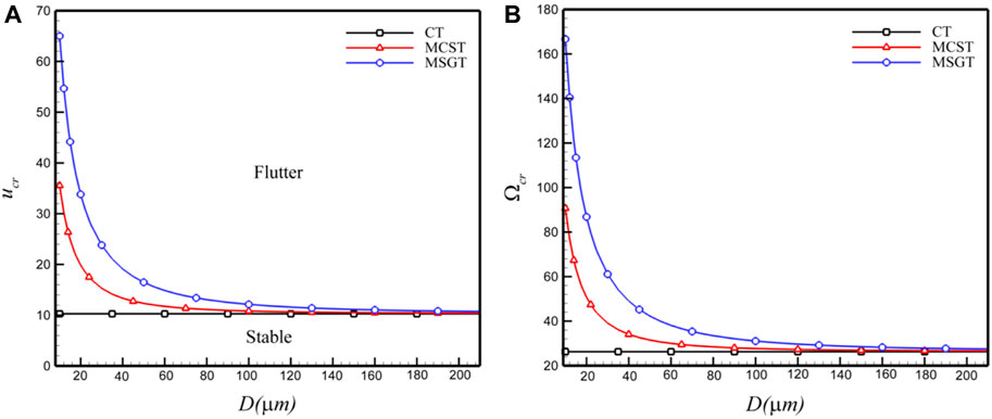
Figure 14. Flutter boundaries as a function of outside diameter D, (A) critical speed and (B) critical frequencies [91].
When the material length parameter is set to
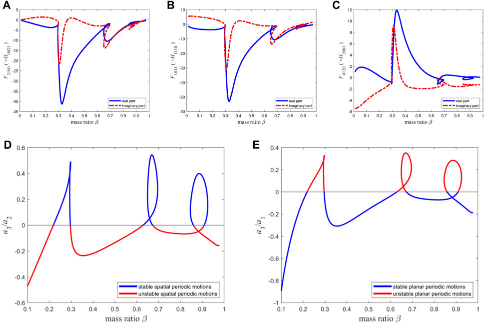
Figure 15. The resonance term coefficients of the second-order discretization equation of the micro pipe with
When the material length parameter is set to
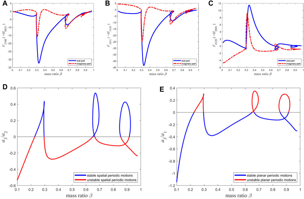
Figure 16. The resonance term coefficients of the second-order discretization equation of the micro pipe with
When
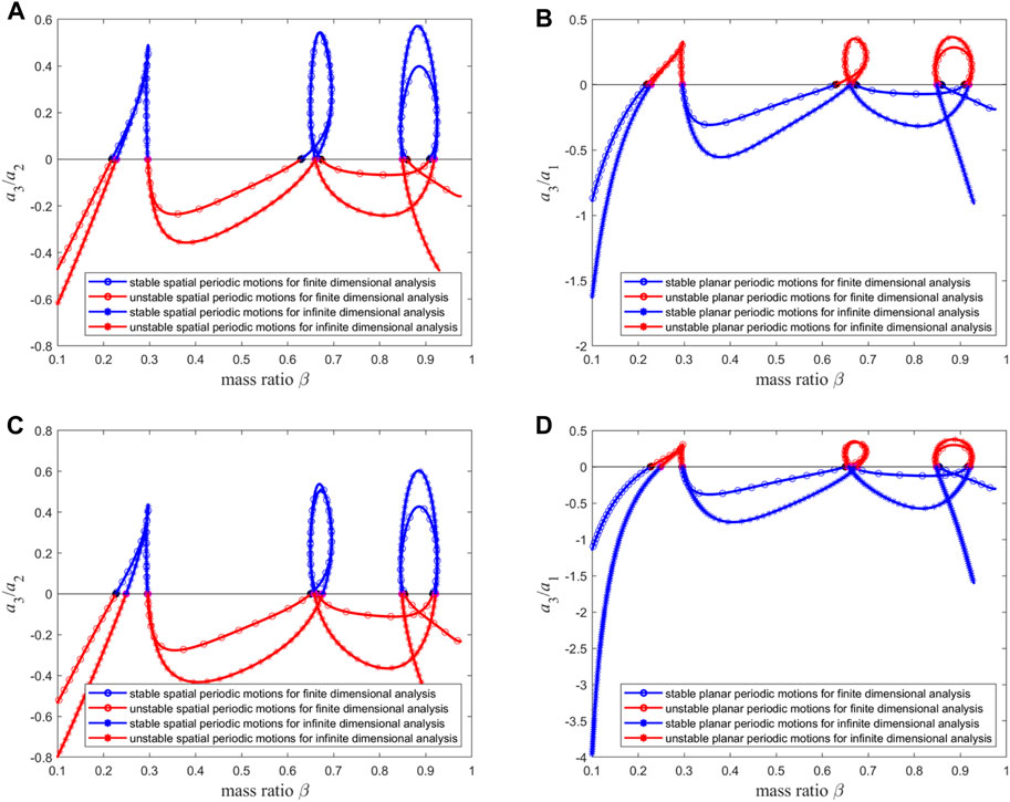
Figure 17. The stabilities of (A) spatial and (B) planar periodic motion for infinite dimensional analysis and finite dimensional analysis with n = 15 when
5 Discussions
When the mode truncation number is set to 15, the stability comparison of the two types of periodic motion for
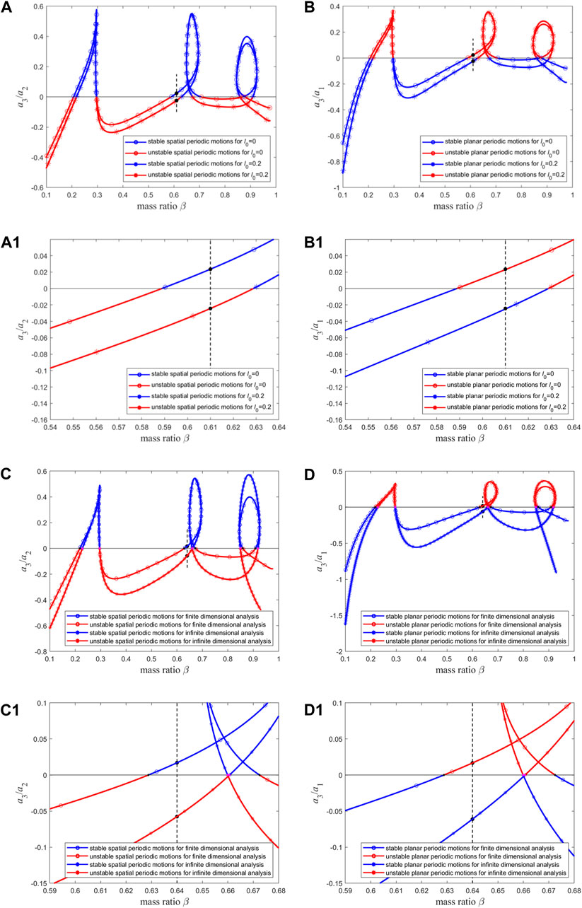
Figure 18. The stabilities of (A) spatial and (B) planar periodic motion for macro pipe (i.e.,
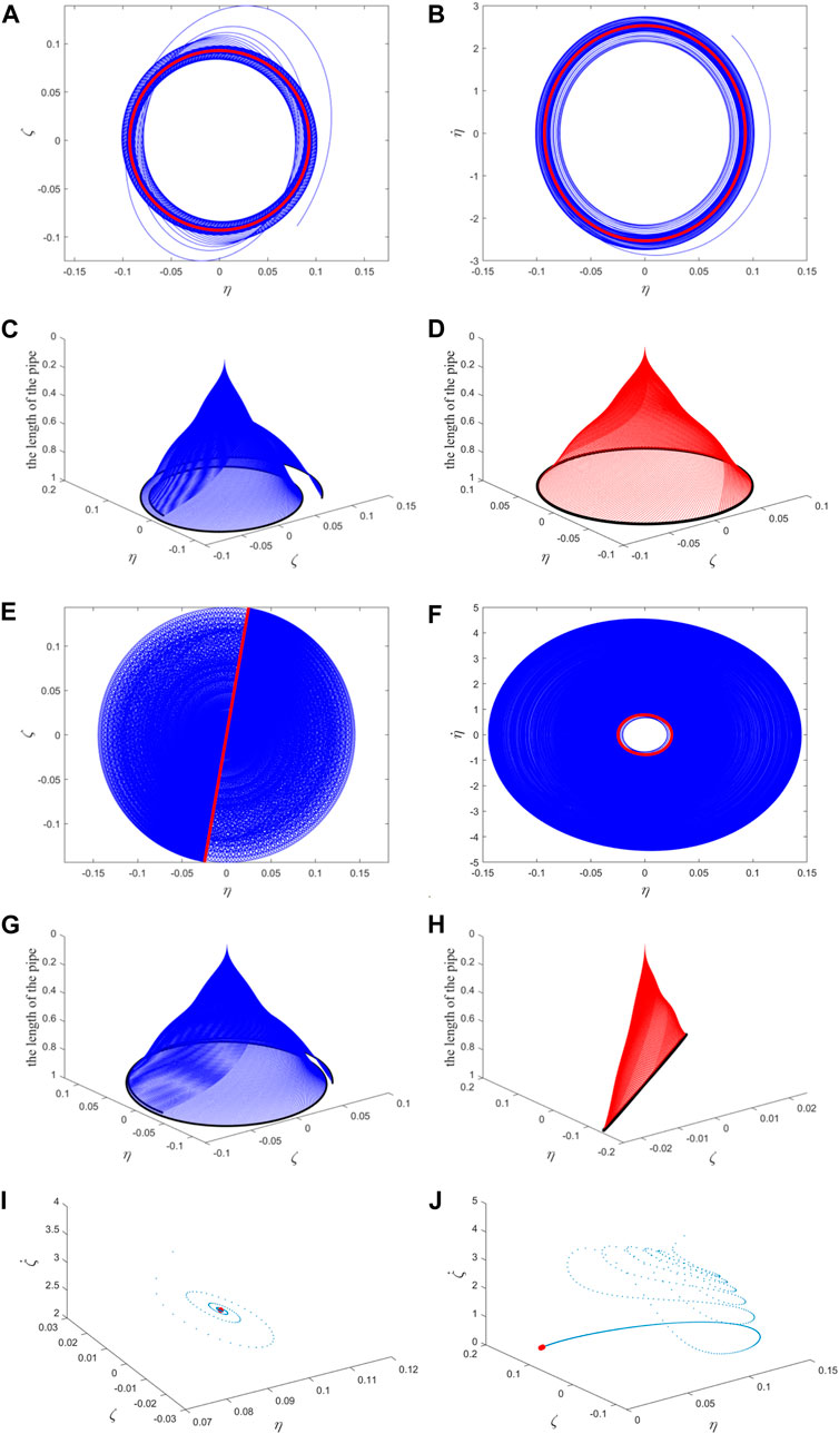
Figure 19. (A) and (E) the position relationship of the free ends of the pipe in two directions; (B) and (F) the velocity-displacement relationship diagram of the free ends of the pipe in one direction; (C) and (G) the transient process of the whole pipe vibration; (D) and (H) the steady-state vibration of the whole pipe. The blue (red) color represents the transient (steady-state) motion in (A–H); The Poincaré map: (I) corresponding to (A–D); (J) corresponding to (E–H). The blue points correspond to transient motion, and the red points correspond to steady-state motion (i.e., fixed point).
According to Eq. 4a, the dimensionless material length scale parameter l0 is positively correlated with the bending stiffness of pipe, which implies that a larger l0 leads to a higher bending stiffness. As shown in Figure 3B, Figure 13A, Figure 3D and Figure 13C larger l0 leads to higher critical flow velocities and frequencies. In summary, a larger bending stiffness leads to higher critical flow velocities and critical frequencies, and makes it more likely for the pipe to exhibit stable planar periodic motion after losing stability.
For the truncated mode numbers n = 9 and n = 11, as shown in Figure 3D, the critical frequencies corresponding to β = 0.725 all are 44.2565. When a small increase in flow velocity causes vibrations as shown in Figures 5J–M, the actual frequency is 45.4974, close to the critical frequency. When a small increase in flow velocity causes vibrations shown in Figures 7F–I, the actual frequency is 45.3660, also close to the critical frequency. This indicates that the vibration frequencies in both Figures 7F–I and Figures 5J–M are near the critical frequency, yet their motion forms differ due to different numbers of mode truncation.
For the truncated mode numbers n = 11 and n = 13, as shown in Figure 3D, the critical frequencies corresponding to β = 0.715 all are 44.0148. When a small increase in flow velocity causes vibrations as shown in Figures 7J–M, the actual frequency is 45.7292, close to the critical frequency. When a small increase in flow velocity causes vibrations shown in Figures 8F–I, the actual frequency is 45.5303, also close to the critical frequency. This indicates that the vibration frequencies in both Figures 8F–I and Figures 7J–M are near the critical frequency, yet their motion forms differ due to different numbers of mode truncation.
For the truncated mode numbers n = 13 and n = 15, as shown in Figure 3D, the critical frequencies corresponding to β = 0.708 all are 43.8340. When a small increase in flow velocity causes vibrations as shown in Figures 8J–M, the actual frequency is 45.8627, close to the critical frequency. When a small increase in flow velocity causes vibrations shown in Figures 9F–I, the actual frequency is 45.6627, also close to the critical frequency. This indicates that the vibration frequencies in both Figures 9F–I and Figures 8J–M are near the critical frequency, yet their motion forms differ due to different numbers of mode truncation.
This paper demonstrates that for a wide range of mass ratio β, the spatial flexural vibrations of the fluid-conveying pipe shown in Figure 1 can be precisely described by the Galerkin discretized ordinary differential equations set of 15 truncated mode numbers. These ordinary differential equations are obtained by discretizing the original motions equations Eq. 4 by using the first 15 mode functions of a cantilever beam, effectively capturing the pipe’s dynamic properties, including critical flow velocity, frequency, amplitude, and motion form. Notably, the types of periodic motion of the pipe (including planar and spatial periodic motions) and their stability can be determined from the coefficients of the Galerkin discretized equations, specifically Eqs 10 and 23, 24, 25, 26, 28, 29, 37. Accurate prediction of the motion form assists in adopting appropriate vibration control measures, whether for stable planar or spatial periodic motions. For instance, stable planar periodic motion may be managed by integrating an energy sink within a specific plane, while managing a stable spatial periodic motion may necessitate the addition of energy sinks encircling the pipe. The projection method used in this paper (based on the Center Manifold-Normal Form Theory) can also be applied to other types of fluid-conveying pipe models, such as those without O (2) symmetry in their cross-sections. However, in such cases, the calculations of the center manifold and reduced-order equations become extremely complex due to the inability to apply ‘symmetry’ to simplifying, it is a matter that the author will seriously consider in future research.
The presence of errors between finite dimensional analysis and infinite dimensional analysis results is proven by taking the mass ratio β = 0.64 and
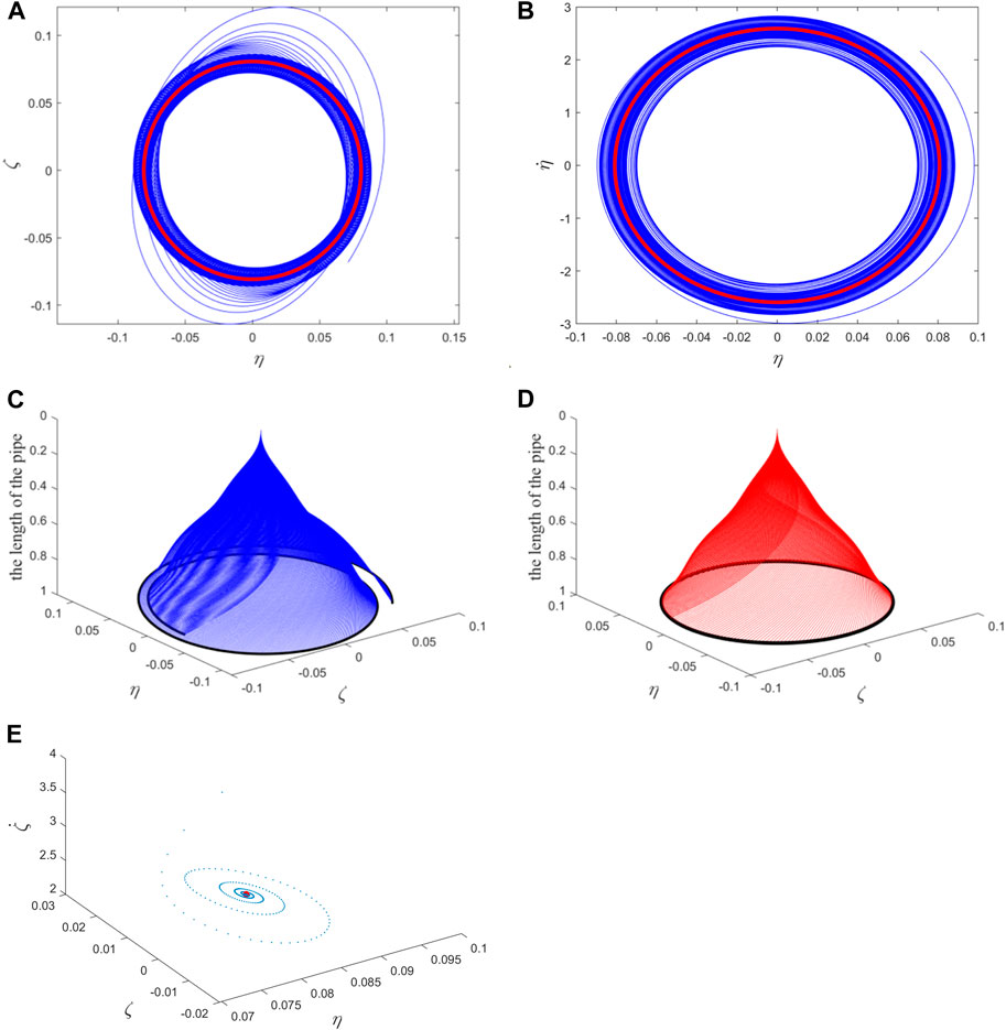
Figure 20. (A) The position relationship of the free ends of the pipe in two directions; (B) the velocity-displacement relationship diagram of the free ends of the pipe in one direction; (C) the transient process of the whole pipe vibration; (D) the steady-state vibration of the whole pipe. The blue (red) color represents the transient (steady-state) motion in (A–D); (E) The Poincaré map corresponding to (A–D). The blue points correspond to transient motion, and the red points correspond to steady-state motion (i.e., fixed point).
Galerkin method is also suitable for motions equations with large nonlinear terms, even though the flow velocity is far away from the instability threshold. Generally, more truncated mode numbers produce more accurate results. However, the center manifold theory and normal form method are applicable only close to the bifurcation point, i.e., for flow velocity not far away from the critical value. This is the limitation of the present reduced two-degree-of-freedom model. When the flow velocity is gradually increased beyond the instability threshold, the types, stabilities, and bifurcations of periodic motions of fluid-conveying cantilevered micropipes, e.g., the occurrence of torus motions or chaos, are still some of the open questions.
In practical applications, two considerations are proposed. Firstly, if the actual pipe model closely resembles that shown in Figure 1, then based on the specific mass ratio β and l0, Eqs 10 and 23, 24, 25, 26, 28, 29, 37 can be calculated to determine the type of motion that the pipe will undergo after instability, either stable planar or spatial periodic motion, thereby selecting appropriate control strategies. Additionally, adjustments to the values of β and l0 can facilitate these two types of motion for the pipe. Secondly, if the actual pipe model differs from that in Figure 1, the numbers of mode truncation n when using Galerkin method should be 15 or more to ensure the convergence of dynamic properties such as critical flow velocity, frequency, amplitude, and motion form.
6 Conclusion
In this study, by using the Galerkin method, the spatial vibration Eq. 4 of the macro- and micro-scale cantilevered fluid-conveying pipe is discretized into a system of ordinary differential Eq. 9. Meanwhile, the reduced-order Eq. 23 of the system of ordinary differential equations and associated coefficients (24) and (25) are calculated with the projection method. Based on this, two types of periodic motion and their stability within the system are investigated. The results of various mode truncation numbers are compared longitudinally and transversely with infinite dimensional analysis results by setting the modal truncation number incrementally. The following conclusions are obtained.
(1) For the linear vibration characteristics of pipes, which includes the critical flow velocity, the critical frequency and the change rate of the real part of the critical eigenvalue, the 9-mode Galerkin discretization equations can obtain results relatively close to those of the infinite dimensional analysis. As shown by Figure 3 and Figure 4. However, the 9-mode Galerkin discretization equations cannot give convergent results for the nonlinear vibration characteristics of pipes.
(2) As the mode truncation number n continues to increase, the results about the nonlinear vibration characteristics of pipes (i.e., the planar and spatial periodic motions) obtained when n = 11 have a minor correction to the results obtained when n = 9; there are similar minor corrections for the results of n = 13 to those of n = 11, results of n = 15 to those of n = 13, until the results of n = 16 are almost the same as those of n = 15. That is, when n = 15, the result converges, so this is a reasonable mode truncation number.
(3) With a mode truncation number of 15, the differences between the results of the finite dimensional and infinite dimensional analysis are calculated for macro- (
Data availability statement
The original contributions presented in the study are included in the article/supplementary material, further inquiries can be directed to the corresponding author.
Author contributions
YG: Writing–original draft, Writing–review and editing, Writing–original draft, Writing–review and editing.
Funding
The author(s) declare that financial support was received for the research, authorship, and/or publication of this article. The supports from the National Natural Science Foundation of China (No, 12002096) and the 2022 Doctoral Foundation of Anshun University (No, asxybsjj202201) are acknowledged.
Conflict of interest
The author declares that the research was conducted in the absence of any commercial or financial relationships that could be construed as a potential conflict of interest.
Publisher’s note
All claims expressed in this article are solely those of the authors and do not necessarily represent those of their affiliated organizations, or those of the publisher, the editors and the reviewers. Any product that may be evaluated in this article, or claim that may be made by its manufacturer, is not guaranteed or endorsed by the publisher.
References
1. Benjamin TB. Dynamics of a system of articulated pipes conveying fluid: I. Theory. Proc R Soc Lond Ser A, Math Phys Sci (1961) 261:457–86.
2. Gregory RW, Païdoussis MP. Unstable oscillation of tubular cantilevers conveying fluid I. Theory. Proc R Soc Lond Ser A. Math Phys Sci (1966) 293:512–27. doi:10.1098/rspa.1966.0187
3. Chen SS. Forced vibration of a cantilevered tube conveying fluid. The J Acoust Soc America (1970) 48:773–5. doi:10.1121/1.1912205
4. Ginsberg JH. The dynamic stability of a pipe conveying a pulsating flow. Int J Eng Sci (1973) 11:1013–24.
5. Païdoussis MP, Issid NT. Dynamic stability of pipes conveying fluid. J Sound Vibration (1974) 33:267–94. doi:10.1016/s0022-460x(74)80002-7
6. Holmes PJ. Bifurcations to divergence and flutter in flow-induced oscillations: a finite dimensional analysis. J Sound Vibration (1977) 53:471–503. doi:10.1016/0022-460x(77)90521-1
7. Holmes PJ. Pipes supported at both ends cannot flutter. J Appl Mech (1978) 45:619–22. doi:10.1115/1.3424371
8. Holmes P, Marsden J. Bifurcation to Divergence and flutter in flow-induced oscillations: an infinite dimensional analysis. Automatica (1978) 14:367–84. doi:10.1016/0005-1098(78)90036-5
9. Rousselet J, Herrmann G. Dynamic behavior of continuous cantilevered pipes conveying fluid near critical velocities. J Appl Mech (1981) 48:943–7. doi:10.1115/1.3157760
10. Namchchivaya NS, Tien WM. Non-linear dynamics of supported pipe conveying pulsating fluid-II. Combination resonance. Int J Non-linear Mech (1989) 24:197–208. doi:10.1016/0020-7462(89)90038-3
11. Jayaraman K, Narayaman S. Chaotic oscillations in pipes conveying pulsating fluid. Nonlinear Dyn (1996) 10:333–57.
12. Namchchivaya NS. Non-linear dynamics of supported pipe conveying pulsating fluid-I. Subharmonic resonance. Int J Non-linear Mech (1989) 24:185–96.
13. Chang CO, Chen KC. Dynamics and stability of pipes conveying fluid. J Press Vessel Technol (1994) 116:57–66. doi:10.1115/1.2929559
14. Li GX, Païdoussis MP. Stability, double degeneracy and chaos in cantilevered pipes conveying fluid. Int J Non-Linear Mech (1994) 29:83–107. doi:10.1016/0020-7462(94)90054-x
15. Païdoussis MP, Li GX, Moon FC. Chaotic oscillations of the autonomous system of a constrained pipe conveying fluid. J Sound Vibration (1989) 135:1–19. doi:10.1016/0022-460x(89)90750-5
16. Païdoussis MP, Semler C. Nonlinear and chaotic oscillations of a constrained cantilevered pipe conveying fluid: a full nonlinear analysis. Nonlinear Dyn (1993) 4:655–70.
17. Jin JD. Stability and chaotic motions of a restrained pipe conveying fluid. J Sound Vibration (1997) 208:427–39. doi:10.1006/jsvi.1997.1195
18. Paidoussis MP, Semler C. Nonlinear dynamics of a fluid-conveying cantilevered pipe with an intermediate spring support. J Fluids Structures (1993) 7:269–98.
19. Païdoussis MP, Semler C. Nonlinear analysis of the parametric resonances of a planar fluid-conveying cantilevered pipe. J Fluids Structures (1996) 10:787–825. doi:10.1006/jfls.1996.0053
20. Jin JD, Zou GS. Bifurcations and chaotic motions in the autonomous system of a restrained pipe conveying fluid. J Sound Vibration (2003) 260:783–805. doi:10.1016/s0022-460x(02)00982-3
21. Jin JD, Song ZY. Parametric resonances of supported pipes conveying pulsating fluid. J Fluids Structures (2005) 20:763–83. doi:10.1016/j.jfluidstructs.2005.04.007
22. Szabό Z. Nonlinear analysis of a cantilever pipe containing pulsatile flow. Meccanica (2003) 38:161–72.
23. Nikolić M, Rajković M. Bifurcations in nonlinear models of fluid-conveying pipes supported at both ends. J Fluids Structures (2006) 22:173–95. doi:10.1016/j.jfluidstructs.2005.09.009
24. Wadham-Gagnon M, Païdoussis MP, Semler C. Dynamics of cantilevered pipes conveying fluid. Part 1: nonlinear equations of three-dimensional motion. J Fluids Structures (2007) 23:545–67. doi:10.1016/j.jfluidstructs.2006.10.006
25. Lundgren TS, Sethna PR, Bajaj AK. Stability boundaries for flow induced motions of tubes with an inclined terminal nozzle. J Sound Vibration (1979) 64:553–71. doi:10.1016/0022-460x(79)90804-6
26. Modarres-Sadeghi Y, Païdoussis MP, Semler C. Three-dimensional oscillations of a cantilever pipe conveying fluid. Int J Non-Linear Mech (2008) 43:18–25. doi:10.1016/j.ijnonlinmec.2007.09.005
27. Païdoussis MP, Semler C, Wadham-Gagnon M, Saaid S. Dynamics of cantilevered pipes conveying fluid. Part 2: dynamics of the system with intermediate spring support. J Fluids Structures (2007) 23:569–87. doi:10.1016/j.jfluidstructs.2006.10.009
28. Modarres-Sadeghi Y, Semler C, Wadham-Gagnon M, Païdoussis MP. Dynamics of cantilevered pipes conveying fluid. Part 3: three-dimensional dynamics in the presence of an end-mass. J Fluids Structures (2007) 23:589–603. doi:10.1016/j.jfluidstructs.2006.10.007
29. Ghayesh MH, Païdoussis MP, Modarres-Sadeghi Y. Three-dimensional dynamics of a fluid-conveying cantilevered pipe fitted with an additional spring-support and an end-mass. J Sound Vibration (2011) 330:2869–99. doi:10.1016/j.jsv.2010.12.023
30. Ghayesh MH, Païdoussis MP. Three-dimensional dynamics of a cantilevered pipe conveying fluid, additionally supported by an intermediate spring array. Int J Non-Linear Mech (2010) 45:507–24. doi:10.1016/j.ijnonlinmec.2010.02.001
31. Modarres-Sadeghi Y, Païdoussis MP. Chaotic oscillations of long pipes conveying fluid in the presence of a large end-mass. Comput Structures (2013) 122:192–201. doi:10.1016/j.compstruc.2013.02.005
32. Chang GH, Modarres-Sadeghi Y. Flow-induced oscillations of a cantilevered pipe conveying fluid with base excitation. J Sound Vibration (2014) 333:4265–80. doi:10.1016/j.jsv.2014.03.036
33. Alsaud H, Alshehri MH. Continuum modeling for lithium storage inside nanotubes. Front Phys (2023) 11. doi:10.3389/fphy.2023.1221720
34. Yun C, Wu Y, Liang Z, Yang W, Du H, Liu S, et al. Magnetic anisotropy-controlled vortex nano-oscillator for neuromorphic computing. Front Phys (2022) 10. doi:10.3389/fphy.2022.1019881
35. Wang Y, Zhang X, Zhou T, Zhu Y, Cui Z, Zhang K. Properties and sensing performance of THz metasurface based on carbon nanotube and microfluidic channel. Front Phys (2021) 9. doi:10.3389/fphy.2021.749501
36. Shephard JD, Urich A, Carter RM, Jaworski P, Maier RRJ, Belardi W, et al. Silica hollow core microstructured fibers for beam delivery in industrial and medical applications. Front Phys (2015) 3. doi:10.3389/fphy.2015.00024
37. Tadi Beni Y, Karimipour I, Abadyan M. Modeling the instability of electrostatic nano-bridges and nano-cantilevers using modified strain gradient theory. Appl Math Model (2015) 39:2633–48. doi:10.1016/j.apm.2014.11.011
38. Arefi M, Zenkour AM. Influence of micro-length-scale parameters and inhomogeneities on the bending, free vibration and wave propagation analyses of a FG Timoshenko’s sandwich piezoelectric microbeam. J Sandwich Structures Mater (2017) 21:1243–70. doi:10.1177/1099636217714181
39. Arefi M, Zenkour AM. Transient analysis of a three-layer microbeam subjected to electric potential. Int J Smart Nano Mater (2017) 8:20–40. doi:10.1080/19475411.2017.1292967
40. Yayli MÖ. Buckling analysis of a microbeam embedded in an elastic medium with deformable boundary conditions. Micro Nano Lett (2016) 11:741–5. doi:10.1049/mnl.2016.0257
41. Karimipour I, Tadi Beni Y, Akbarzadeh AH. Modified couple stress theory for three-dimensional elasticity in curvilinear coordinate system: application to micro torus panels. Meccanica (2020) 55:2033–73. doi:10.1007/s11012-020-01220-3
42. Arefi M, Moghaddam SK, Bidgoli EM-R, Kiani M, Civalek O. Analysis of graphene nanoplatelet reinforced cylindrical shell subjected to thermo-mechanical loads. Compos Structures (2021) 255:112924. doi:10.1016/j.compstruct.2020.112924
43. Heidari Y, Arefi M, Irani Rahaghi M. Nonlocal vibration characteristics of a functionally graded porous cylindrical nanoshell integrated with arbitrary arrays of piezoelectric elements. Mech Based Des Structures Machines (2020) 50:4246–73. doi:10.1080/15397734.2020.1830799
44. Mohammadi M, Arefi M, Dimitri R, Tornabene F. Higher-order thermo-elastic analysis of FG-CNTRC cylindrical vessels surrounded by a pasternak foundation. Nanomaterials (2019) 9:79. doi:10.3390/nano9010079
45. Zeighampour H, Beni YT, Karimipour I. Wave propagation in double-walled carbon nanotube conveying fluid considering slip boundary condition and shell model based on nonlocal strain gradient theory. Microfluidics and Nanofluidics (2017) 21:85. doi:10.1007/s10404-017-1918-3
46. Yang T-Z, Ji Sd., Yang X-D, Fang B. Microfluid-induced nonlinear free vibration of microtubes. Int J Eng Sci (2014) 76:47–55. doi:10.1016/j.ijengsci.2013.11.014
47. Dai HL, Wang L, Abdelkefi A, Ni Q. On nonlinear behavior and buckling of fluid-transporting nanotubes. Int J Eng Sci (2015) 87:13–22. doi:10.1016/j.ijengsci.2014.11.005
48. Bahaadini R, Hosseini M. Nonlocal divergence and flutter instability analysis of embedded fluid-conveying carbon nanotube under magnetic field. Microfluidics and Nanofluidics (2016) 20:108. doi:10.1007/s10404-016-1773-7
49. Bahaadini R, Hosseini M. Effects of nonlocal elasticity and slip condition on vibration and stability analysis of viscoelastic cantilever carbon nanotubes conveying fluid. Comput Mater Sci (2016) 114:151–9. doi:10.1016/j.commatsci.2015.12.027
50. Hu K, Wang YK, Dai HL, Wang L, Qian Q. Nonlinear and chaotic vibrations of cantilevered micropipes conveying fluid based on modified couple stress theory. Int J Eng Sci (2016) 105:93–107. doi:10.1016/j.ijengsci.2016.04.014
51. Dai H-L, Wu P, Wang L. Nonlinear dynamic responses of electrostatically actuated microcantilevers containing internal fluid flow. Microfluidics and Nanofluidics (2017) 21:162. doi:10.1007/s10404-017-1999-z
52. Ghayesh MH, Farokhi H, Farajpour A. Chaotic oscillations of viscoelastic microtubes conveying pulsatile fluid. Microfluidics and Nanofluidics (2018) 22:72. doi:10.1007/s10404-018-2091-z
53. Zhu B, Chen X, Dong Y, Li Y. Stability analysis of cantilever carbon nanotubes subjected to partially distributed tangential force and viscoelastic foundation. Appl Math Model (2019) 73:190–209. doi:10.1016/j.apm.2019.04.018
54. Sarparast H, Alibeigloo A, Kesari SS, Esfahani S. Size-dependent dynamical analysis of spinning nanotubes conveying magnetic nanoflow considering surface and environmental effects. Appl Math Model (2022) 108:92–121. doi:10.1016/j.apm.2022.03.017
55. Bajaj AK, Sethna PR, Lundgren TS. Hopf bifurcation phenomena in tubes carrying a fluid. Soc Ind Appl Maths (1980) 39:213–30. doi:10.1137/0139019
56. Bajaj AK. Bifurcations in a parametrically excited non-linear oscillator. Int J Non-Linear Mech (1987) 22:47–59. doi:10.1016/0020-7462(87)90048-5
57. Bajaj AK, Sethna PR. Flow induced bifurcations to three-dimensional oscillatory motions in continuous tubes, Society for Industrial and Applied Mathematics. J Appl Maths (1984) 44:270–86.
58. Bajaj AK, Sethna PR. Effect of symmetry-breaking perturbations on flow-induced oscillations in tubes. J Fluids Structures (1991) 5:651–79. doi:10.1016/0889-9746(91)90344-o
59. Folley CN, Bajaj AK. Spatial nonlinear dynamics near principal parametric resonance for a fluid-conveying cantilever pipe. J Fluids Structures (2005) 21:459–84. doi:10.1016/j.jfluidstructs.2005.08.014
60. Yamashita K, Yagyu T, Yabuno H. Nonlinear interactions between unstable oscillatory modes in a cantilevered pipe conveying fluid. Nonlinear Dyn (2019) 98:2927–38. doi:10.1007/s11071-019-05236-7
61. Yamashita K, Nishiyama N, Katsura K, Yabuno H. Hopf-Hopf interactions in a spring-supported pipe conveying fluid. Mech Syst Signal Process (2021) 152:107390. doi:10.1016/j.ymssp.2020.107390
62. Yamashita K, Kitaura K, Nishiyama N, Yabuno H. Non-planar motions due to nonlinear interactions between unstable oscillatory modes in a cantilevered pipe conveying fluid. Mech Syst Signal Process (2022) 178:109183. doi:10.1016/j.ymssp.2022.109183
63. Furuya H, Yamashita K, Yabuno H. Nonlinear stability of a fluid-conveying cantilevered pipe with end mass in case of horizontal excitation at the upper end. Proc ASME 2010 3rd Jt US-European Fluids Eng Summer Meet 8th Int Conf Nanochannels, Microchannels, Minichannels (2010) 1–9. doi:10.1115/FEDSM-ICNMM2010-31239
64. Zhang L-x., Huang W-h. ANALYSIS OF NONLINEAR DYNAMIC STABILITY OF LIQUID-CONVEYING PIPES. Appl Maths Mech (2002) 23:1071–80.
65. Amiri A, Masoumi A, Talebitooti R. Flutter and bifurcation instability analysis of fluid-conveying micro-pipes sandwiched by magnetostrictive smart layers under thermal and magnetic field. Int J Mech Mater Des (2020) 16:569–88. doi:10.1007/s10999-020-09487-w
66. Jin Q, Ren Y. Nonlinear size-dependent bending and forced vibration of internal flow-inducing pre- and post-buckled FG nanotubes. Commun Nonlinear Sci Numer Simulation (2022) 104:106044. doi:10.1016/j.cnsns.2021.106044
67. Jin Q, Ren Y. Dynamic instability mechanism of post-buckled FG nanotubes transporting pulsatile flow: size-dependence and local/global dynamics. Appl Math Model (2022) 111:139–59. doi:10.1016/j.apm.2022.06.025
68. Jin Q, Ren Y, Yuan F-G. Combined resonance of pulsatile flow-transporting FG nanotubes under forced excitation with movable boundary. Nonlinear Dyn (2022) 111:6157–78. doi:10.1007/s11071-022-08148-1
69. Chehreghani M, Shaaban A, Misra AK, Païdoussis MP. Experimental investigation of the dynamics of slightly curved cantilevered pipes conveying fluid. Nonlinear Dyn (2023) 111:22101–17. doi:10.1007/s11071-023-08384-z
70. Guo Y, Xie Jh., Wang L. Three-dimensional vibration of cantilevered fluid-conveying micropipes—types of periodic motions and small-scale effect. Int J Non-Linear Mech (2018) 102:112–35. doi:10.1016/j.ijnonlinmec.2018.04.001
71. Guo Y. Periodic motion of microscale cantilevered fluid-conveying pipes with symmetric breaking on the cross-section. Appl Math Model (2023) 116:277–326. doi:10.1016/j.apm.2022.11.023
72. Ma Y, You Y, Chen K, Hu L, Feng A. Application of harmonic differential quadrature (HDQ) method for vibration analysis of pipes conveying fluid. Appl Maths Comput (2023) 439:127613. doi:10.1016/j.amc.2022.127613
73. Mao X-Y, Jing J, Ding H, Chen L-Q. Dynamics of axially functionally graded pipes conveying fluid. Nonlinear Dyn (2023) 111:11023–44. doi:10.1007/s11071-023-08470-2
74. Arefi M, Karroubi R, Irani-Rahaghi M. Free vibration analysis of functionally graded laminated sandwich cylindrical shells integrated with piezoelectric layer. Appl Maths Mech (2016) 37:821–34. doi:10.1007/s10483-016-2098-9
75. Arefi M, Faegh RK, Loghman A. The effect of axially variable thermal and mechanical loads on the 2D thermoelastic response of FG cylindrical shell. J Therm Stresses (2016) 39:1539–59. doi:10.1080/01495739.2016.1217178
76. Arefi M, Abbasi AR, Vaziri Sereshk MR. Two-dimensional thermoelastic analysis of FG cylindrical shell resting on the Pasternak foundation subjected to mechanical and thermal loads based on FSDT formulation. J Therm Stresses (2016) 39:554–70. doi:10.1080/01495739.2016.1158607
77. Arefi M, Rahimi GH. The effect of nonhomogeneity and end supports on the thermo elastic behavior of a clamped–clamped FG cylinder under mechanical and thermal loads. Int J Press Vessels Piping (2012) 96-97:30–7. doi:10.1016/j.ijpvp.2012.05.009
78. Saeedi S, Kholdi M, Loghman A, Ashrafi H, Arefi M. Thermo-elasto-plastic analysis of thick-walled cylinder made of functionally graded materials using successive approximation method. Int J Press Vessels Piping (2021) 194:104481. doi:10.1016/j.ijpvp.2021.104481
79. Loghman A, Nasr M, Arefi M. Nonsymmetric thermomechanical analysis of a functionally graded cylinder subjected to mechanical, thermal, and magnetic loads. J Therm Stresses (2017) 40:765–82. doi:10.1080/01495739.2017.1280380
80. Yayli MÖ. A compact analytical method for vibration of micro-sized beams with different boundary conditions. Mech Adv Mater Structures (2016) 24:496–508. doi:10.1080/15376494.2016.1143989
81. Semler C, Li GX, Païdoussis MP. The non-linear equations of motion of pipes conveying fluid. J Sound Vibration (1994) 169:577–99.
82. Yang F, Chong ACM, Lam DCC, Tong P. Couple stress based strain gradient theory for elasticity. Int J Sol Structures (2002) 39:2731–43. doi:10.1016/s0020-7683(02)00152-x
83. Xu J, Wang L. Dynamics and control of fluid-conveying pipe systems. Beijing: Science Press (2015).
84. Dehsaraji ML, Arefi M, Loghman A. Size dependent free vibration analysis of functionally graded piezoelectric micro/nano shell based on modified couple stress theory with considering thickness stretching effect. Defence Technol (2021) 17:119–34. doi:10.1016/j.dt.2020.01.001
85. Beni YT, Karimipöur I, Abadyan M. Modeling the effect of intermolecular force on the size-dependent pull-in behavior of beam-type NEMS using modified couple stress theory. J Mech Sci Technol (2014) 28:3749–57. doi:10.1007/s12206-014-0836-5
86. Karimipour I, Beni YT, Akbarzadeh AH. Size-dependent nonlinear forced vibration and dynamic stability of electrically actuated micro-plates. Commun Nonlinear Sci Numer Simulation (2019) 78:104856. doi:10.1016/j.cnsns.2019.104856
87. Yayli MÖ. Free longitudinal vibration of a nanorod with elastic spring boundary conditions made of functionally graded material. Micro Nano Lett (2018) 13:1031–5. doi:10.1049/mnl.2018.0181
88. Yayli MÖ. Axial vibration analysis of a Rayleigh nanorod with deformable boundaries. Microsystem Tech (2020) 26:2661–71. doi:10.1007/s00542-020-04808-7
89. Yayli MÖ. Free vibration analysis of a rotationally restrained (FG) nanotube. Microsystem Tech (2019) 25:3723–34. doi:10.1007/s00542-019-04307-4
90. Wang Y, Tang M, Yang M, Qin T. Three-dimensional dynamics of a cantilevered pipe conveying pulsating fluid. Appl Math Model (2023) 114:502–24. doi:10.1016/j.apm.2022.10.023
91. Hosseini M, Bahaadini R. Size dependent stability analysis of cantilever micro-pipes conveying fluid based on modified strain gradient theory. Int J Eng Sci (2016) 101:1–13. doi:10.1016/j.ijengsci.2015.12.012
92. Kuznetsov YA. Elements of applied bifurcation theory. 3rd ed. ed. New York: Springer-Verlag (2004).
93. Lam DCC, Yang F, Chong ACM, Wang J, Tong P. Experiments and theory in strain gradient elasticity. J Mech Phys Sol (2003) 51:1477–508. doi:10.1016/s0022-5096(03)00053-x
94. McFarland AW, Colton JS. Role of material microstructure in plate stiffness with relevance to microcantilever sensors. J Micromechanics Microengineering (2005) 15:1060–7. doi:10.1088/0960-1317/15/5/024
Keywords: fluid-conveying pipe, reduced-order equations, finite dimensional analysis, infinite dimensional analysis, periodic motion, Galerkin discretization
Citation: Guo Y (2024) Periodic motion of macro- and/or micro-scale cantilevered fluid-conveying pipes with O(2) symmetry: a finite dimensional analysis. Front. Phys. 12:1342425. doi: 10.3389/fphy.2024.1342425
Received: 21 November 2023; Accepted: 18 March 2024;
Published: 01 May 2024.
Edited by:
Chun-Hui He, Xi’an University of Architecture and Technology, ChinaReviewed by:
Iman Karimipour, McGill University, CanadaMustafa Özgür Yayli, Bursa Uludağ University, Türkiye
Copyright © 2024 Guo. This is an open-access article distributed under the terms of the Creative Commons Attribution License (CC BY). The use, distribution or reproduction in other forums is permitted, provided the original author(s) and the copyright owner(s) are credited and that the original publication in this journal is cited, in accordance with accepted academic practice. No use, distribution or reproduction is permitted which does not comply with these terms.
*Correspondence: Yong Guo, Z3ktZ2F0ZXNAMTYzLmNvbQ==