On the calculation of irregular solutions of the Schrödinger equation for non-spherical potentials with applications to metallic alloys

Abstract

The irregular solutions of the stationary Schrödinger equation are important for the fundamental formal development of scattering theory. They are also necessary for the analytical properties of the Green function, which in practice can greatly speed up calculations. Nevertheless, they are seldom considered in numerical treatments because of their divergent behavior at origin. This divergence demands high numerical precision that is difficult to achieve, particularly for non-spherical potentials which lead to different divergence rates in the coupled angular momentum channels. Based on an unconventional treatment of boundary conditions, an integral-equation method is here developed which is capable of dealing with this problem. The available precision is illustrated by electron-density calculations for NiTi in its monoclinic B19’ structure.

1 Introduction

The problem of the numerical solution of the stationary Schrödinger equation for a single particle has been investigated in very many scientific publications but rarely with a focus on irregular solutions. While, for spherical potentials, the separation of radial and angular variables simplifies the problem into the solution of one-dimensional radial Schrödinger equations, the situation is more complicated for non-spherical potentials. Here, the separation of variables leads to radial equations where different angular momentum components are coupled by the non-diagonal potential matrix elements. If, as usual, a cutoff is applied by restricting angular-momentum components to , then independent second-order linear differential equations must be solved for spherical potentials, while a set of coupled second-order linear differential equations must be solved for non-spherical potentials. This represents a significant complication, particularly for the irregular solutions, which diverge with different powers of the radial variable as .

It is the purpose of this paper to present an approach which is capable of treating the divergent behavior in a numerically efficient manner. The approach is based on the integral-equation method of Gonzales et al. [1], who obtained regular solutions of the radial Schrödinger by integrations using Clenshaw–Curtis quadratures [2]. The numerical solution of second-order differential equations by integral-equation methods was introduced by Greengard [3] and Greengard and Rokhlin [4], who observed that stable, high-order numerical methods exist for the solution of integral equations. For instance, evaluation of the integrals with Clenshaw–Curtis quadratures leads to spectral accuracy. Spectral accuracy means that the results converge with the inverse th power of the number of mesh points for -times continuously differentiable integrands and exponentially for . In contrast to this, the accuracy of solutions of differential equations by finite difference methods, like the Numerov method used in [5], is limited by a small inverse power of the number of mesh points.

The paper is organized as follows. In Section 2, the mathematical approach is presented. First, the integral equations for the coupled radial equations are defined and their boundary conditions are discussed. Then, we explain how the numerical effort can be reduced by using auxiliary integral equations and how discretization at Chebyshev collocation points leads to systems of linear algebraic equations which can be solved by standard numerical techniques. In Section 3, two examples are numerically investigated: a constant potential, for which the results are compared to the analytical results derived from the expressions given in Appendix A, and a realistic potential as it appears in all-electron density-functional electronic-structure calculations. It is shown that accurate bound-state wavefunctions and energies are obtained for constant potentials and that straightforward complex-contour integrations for calculating the electron density from the Green function can be applied. For that purpose, the correct divergence of the Green function at the origin is enforced by using unconventional boundary conditions. The numerical investigations are done with the KKRnano code of the JuKKR code package. This code is based on the full-potential screened Korringa–Kohn–Rostoker Green function method [6] and was developed for density-functional calculations for systems with thousands of atoms [7].

2 Mathematical approach

2.1 Coupled radial equations

The coupled regular and irregular solutions of the Schrödinger equationfor the potential can be defined [8] by linear Fredholm integral equations of the second kind asand asHereare matrix elements of the potential andis a matrix, which implicitly depends on the irregular solutions. The function is given byIn these equations and throughout the paper, Rydberg atomic units are used. , , and are spherical Bessel, Hankel, and Neumann functions, spherical harmonics, and a combined index for the angular momentum quantum numbers and , respectively. Radial and angular variables are denoted by and , respectively, and is the square root of the energy variable.

The important difference between the inhomogeneous integral Eq. 2 for the regular solutions and Eq. 3 for the irregular solutions is that the source term in Eq. 2 contains Bessel functions, which lead to the behavior of the regular solutions at the origin. The source term in Eq. 3 contains Hankel functions, which lead to the behavior of the irregular solutions at the origin. The numerical solution of Eq. 3 demands high accuracy because the integrand contains functions which increase with different powers  at the origin.

If, as is often done, the coupled radial solutions are not determined from the Fredholm integral Eqs 2, 3 but from differential equations, an additional difficulty arises. The differential equations can be obtained from Eqs 2, 3 by applying the operatorWith , , and , this leads to the coupled Schrödinger equationsfor the regular solutions and to an identical equation for the irregular solutions . With the cutoff , the differential equation Eq. 8 has linearly independent solutions—one regular and one irregular solution for each value of . The different solutions are distinguished by different boundary conditions. These conditions must be specified explicitly for the differential equation (Eq. 8) while they are naturally contained in the integral equations (Eqs 2, 3) as a consequence of the source terms. During the numerical solution of the differential equation (Eq. 8), it is essential to maintain the linear independence of the solutions. Because of the discretization error, this represents a considerable challenge already for the regular solutions, for instance, as explained in [9], and an even greater challenge for the irregular solutions because these diverge at the origin. A discretization error, of course, also occurs in numerical treatments of integral equations, but by using Clenshaw–Curtis quadrature, the error can be made substantially smaller so that accurate results can be achieved.

2.2 Boundary conditions

To discuss the boundary conditions, it is convenient to assume finite integration limits and . This is equivalent to the assumption that the potential vanishes for and . For such potentials, the integral equation Eq. 3 can be written aswhere Eq. 6 was used. Withwhich arises from Eq. 5 for the finite integration limits, Eq. 9 for can be rewritten asThis shows that the irregular solutions can be expressed aswhere the matrix functions and are defined asand asFrom Eq. 12, the inner and outer boundary conditions are obtained as

Like Eq. 12, the regular solutions can be expressed aswith matrix functions and defined asand asThis can be shown by using Eq. 6 in Eq. 2, which results inFrom Eq. 16, the inner and outer boundary conditions are obtained as

2.3 Auxiliary integral equations

The use of integral equations instead of differential equations has been hindered in the past by the much larger computational work. When the interval from to is discretized by mesh points, the integral equations given above can be converted into systems of linear algebraic equations with the dimension . Thus, the computing time scales as whereas the computing time to solve linear differential equations typically scales only linearly with . This means that the effort increases with the third power of the interval length for the solution of linear integral equations, but only linearly with for the solution of linear differential equations.

To overcome this problem, Greengard and Rokhlin [4] observed that the cubic scaling with is avoided by dividing the interval into subintervals and by solving auxiliary integral equations locally in each subinterval. If the interval is divided into subintervals with and and if discretization points are used in each subinterval, the computing time scales as for the solution of the auxiliary integral equations. Thus, it increases only linearly with the interval length . Admittedly, the prefactor can be large, but this is not a serious drawback in view of current computer capabilities. The method of subintervals is based on the property that the integral equation Eq. 11 for the coupled irregular solutions can be written aswhere the matrix function (Eqs 13, 14) are used for the particular value and the integrals arise from deviations of the matrix functions at and . The idea is to solve Eq. 21 separately for each subinterval with restricted as by introducing auxiliary integral equationsandThe advantage of introducing these local solutions is that they do not depend on the unknown solution , unlike Eq. 21 which contains the matrix functions Eq. 13 and Eq. 14. With the local solutions, which can be obtained numerically as described in Section 2.5, the irregular solution can be expressed in the interval asThis can be verified by multiplying Eq. 22 with and Eq. 23 with , which yieldsAdding Eqs 25, 26 both multiplied with and summed over , leads to an integral equation which, compared with Eq. 21, contains the same source term and kernel. Thus, the left and right sides of Eq. 24 represent the same function.

It remains to calculate the matrix functions given by Eqs 13, 14 at the subinterval boundaries . This can be done recursively by recognizing that these functions satisfy the expressionsandand by using Eq. 24, which shows that the function can be expressed by the local solutions and . This leads to the integralswhich must be evaluated numerically as described in Section 2.5. By using Eqs 29–32 the expressions (Eqs 27, 28) can be written as recursion relationsstarting from and .

The method of subintervals is particularly advantageous for potentials with a finite number of discontinuities in the radial direction. Such discontinuities arise, for instance, in full-potential Korringa–Kohn–Rostoker calculations where the angular integration in Eq. 4 must be cut off at boundaries of the atomic cells, which leads to jumps in the radial derivative of the matrix elements of the potential. If the interval boundaries are adapted to the discontinuities, the discontinuous behavior is treated without numerical approximations, which means that numerical errors only depend on the smoothness of the potential within the intervals. The method of subintervals is also advantageous from a computational point of view because the auxiliary functions Eqs 22, 23 and then the integrals in Eqs 29–32 can be calculated efficiently on multi-core processors separately for each value of .

2.4 Modified boundary conditions

In order to understand the necessity of modified boundary conditions for accurate density calculations, it is useful to consider the complex-contour integralwhich is used to calculate the density from the Green function for the Schrödinger equation (Eq. 1). Here, is the Fermi energy, which determines the total charge and a positive infinitesimal imaginary quantity, which is used to avoid the singularities which exist for real values of . Around each atomic position, the Green function can be written aswhere is given by . The matrix function consists of two contributions, so-called “single-scattering” and “multiple-back-scattering” parts. While the back-scattering part is determined by coupled regular solutions alone, the single-scattering part contains the divergent irregular solutions in the form [8]:Here, and are defined as and , respectively. The effectiveness of the contour integral Eq. 35 arises from the fact that the contour can be chosen in the upper half of the complex- plane, where the integrand is an analytical function of , such that with only 20–30 mesh points on the contour [10], highly accurate density results are obtained even for large systems with many thousands of atoms.

Unfortunately, for the contour integral in Eq. 35, the irregular solutions are absolutely necessary to maintain the analytical behavior of the Green function as discussed in [11]. In a numerical treatment with the standard boundary conditions Eqs 15–20, the divergent behavior of the matrix function is given byfor . The correct behavioris obtained from Eq. 80 derived in Appendix A. Comparison of Eqs 38, 39 shows that the transpose of the matrix must be equal to the inverse of the matrix . Numerically, this cannot be achieved because two different integral equations (Eqs 2, 3) are used to calculate these matrices. A solution for this problem is to apply modified irregular and regular solutions defined asThese solutions have the inner boundary conditionsandfor such that the divergent part of the matrix functionhas the correct behavior given in Eq. 39.

The modified irregular solutions can be calculated bywhich is obtained from Eq. 24 by multiplication with the matrix from the right. The matrices and , which are given byand bysatisfy the recursion relations Eqs 33, 34 with and replaced by and . The only difference is that the starting values are changed from and to and .

The disadvantage of the recursion for and is that the matrix is known only approximately, for instance, by using the numerically obtained result for . This minor problem, however, is offset by the significant advantage that the error is known, which arises from the inaccuracy of , from the numerical approximations necessary to solve the auxiliary integral equations and from roundoff errors. This error is given by the difference between , which is the numerical result obtained after the recursion, and , which is the exact result for . The knowledge of can be used in a second recursion starting from a better approximation for given as the product of and the inverse of . Further improved recursions can be added. In the present study, where electron densities up to were considered, rapid convergence was observed, and no more than two or three passes through the recursion were necessary.

While the straightforward use of repeated recursions for and successfully deals with numerical approximations, the problem of roundoff errors requires modification of the recursion relations such that not butis calculated directly. The modified recursion relations given bylead to a matrix with norm such that the required inverse of can be calculated reliably as . If necessary, further reduction of can be achieved by evaluating Eqs 49, 50 with extended precision.

2.5 Numerical treatment

The integral-equation method of Greengard [3], Greengard and Rokhlin [4], and Gonzales et al. [1] is based on expansions of the potential and solutions of the local integral equations (Eqs 22, 23) in Chebyshev polynomials . The method uses the property that the integralof a functioncan be evaluated at the collocation pointsby matrix multiplicationThe collocation points are the zeros of the Chebyshev polynomial . The matrix is given by the product where and are the “discrete cosine–transform” and “right spectral integration” matrices. The discrete cosine–transform matrix, which is given byconnects the coefficients of the Chebyshev series Eq. 52 with values of the function at the zeros Eq. 53 byThe right spectral integration matrix given in [1] connects the coefficients of the Chebyshev serieswith the coefficients byIn Eq. 57, the -th coefficient is neglected, which is justified because of the fast decay of with increasing for sufficiently smooth functions. The matrix has the non-zero elements , , , and, for , the non-zero elements , , and . These values can be obtained by using the integration rules for Chebyshev polynomials. By using Eq. 54, the local integral equations (Eq. 22) are approximated bywhere the factor comes from the substitution , which transforms the interval into . The matrix is given byThe system Eq. 59 of linear equations can be efficiently solved by standard linear algebra software. It has dimension and requires a computing effort that scales as .

While, in principle, the subintervals can be chosen arbitrarily, the choice should be adapted to the divergent behavior of the irregular solutions for . A suitable choice is given by the prescription with . The transformation to the standard expansion interval is obtained by the substitution . For inverse powers of , the substitution leads towith . Here, the integrand and the integration limits for the integral over do not depend on . Thus, without changing the Chebyshev-expansion order, the same relative accuracy is obtained for all intervals.

3 Numerical investigation

The numerical performance is investigated for two examples: a constant potential, which is analytically solvable, and a realistic non-spherical potential, which is obtained by density-functional electronic-structure calculations for an ordered nickel–titanium alloy. It is shown for the constant potential that accurate bound-state energies and wavefunctions can be obtained from the irregular solutions calculated by the integral-equation approach and that the error of calculated bound-state energies decreases exponentially with the order of the Chebyshev expansion. For the NiTi alloy, it is shown that the irregular solutions obtained can be used in complex-contour integrations to calculate the density from the full-potential multiple-scattering Green function. Thus, such calculations can be performed straightforwardly for systems with many atoms in contrast to other treatments suggested in the past [11–13], which are rather elaborate and unlikely to be useful for systems with more than a few atoms.

3.1 Bound states for a constant potential

The standard method for calculating bound states is based on the property that regular solutions of the Schrödinger equation vanish at infinity if they are evaluated for the correct bound-state energy. For trial energies, the differential equation is solved from the inside, starting with the correct power at , and from the outside starting with 0 at a large value of . The bound-state energy and wavefunction are found if, for the chosen trial energy, the logarithmic derivatives of both solutions continuously match at an intermediate value of . The alternative method suggested here is based on the property that irregular solutions of the Schrödinger equation vanish at the origin if they are evaluated for the correct bound-state energy. For a constant potential, because of its spherical symmetry, the irregular solutions are decoupled and the inner boundary condition Eq. 15 contains diagonal matrices and . The condition for a bound state is then given by which eliminates the diverging Hankel functions in Eq. 15 for . In mathematical scattering theory, the functionis known as the “Jost function.” Its analytical properties in the complex- plane are comprehensively discussed in [14], where it is explained that bound states correspond to zeros of for values on the positive imaginary axis. The determination of these zeros is a one-dimensional root-finding problem treated here by Ridders’ method [15].

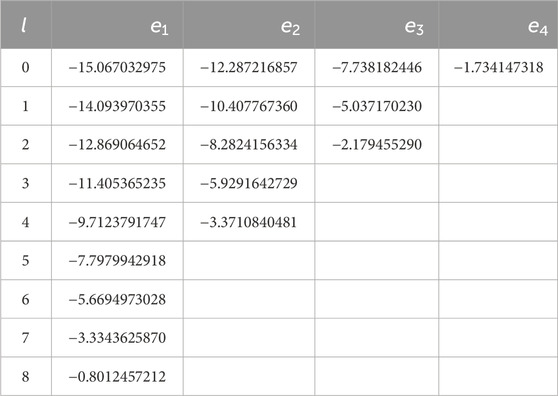
Numerical results for bound-state energies and wavefunctions are shown in Table 1 and Figure 1 for an attractive potential Ry, which is confined to a spherical shell between and . This potential has bound states up to . The energies in Table 1 were obtained using intervals of equal length and order for the Chebyshev expansions. They deviate by less than from the exact energies determined from the zeros of using the analytical expressions given in Appendix A. For comparison with values given in the literature, for example, in [16] where the same potential is treated by sinc-interpolants for , it is useful to know that the same digits as in Table 1 are obtained if is chosen smaller than . This is a consequence of the third-order dependence on , which can be established from the expressions derived in Appendix A.

FIGURE 1

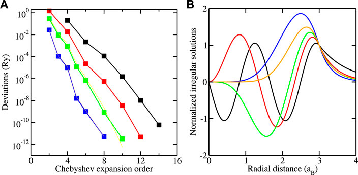
Figure 1 shows how the energy of the lowest bound state for converges with the order of the Chebyshev expansion. The convergence is very similar for the other bound states. The deviations decrease exponentially with the order, and accurate results are already obtained with a small number of intervals by using a sufficiently large order. A precision of is achieved for intervals and order , leading to 45 collocation points. For a larger number of intervals, where a smaller order gives the same precision, more collocation points are necessary. This is, however, not important for the computational effort, which scales as , so that the effects of an increase of and a decrease are practically canceled.

Figure 1 also shows the irregular solutions for the highest bound-state energies for selected values of calculated with and . For the presentation, they are multiplied with and normalized to 1 at . They exponentially decay for and, as a consequence of , regular at . Thus, they satisfy the requirements specifying bound-state wavefunctions. It should be noted that, unlike the example shown, the condition is not always obtained numerically with sufficient precision to conceal the divergent behavior at . It is then more appropriate to determine the bound-state wavefunction not from the irregular solution but from the regular solution by using the property that irregular and regular solutions are multiples of one another at the bound-state energy, as discussed in [14].

3.2 Electron density for NiTi

Metallic alloys of nickel and titanium have interesting and technologically important mechanical properties, like the shape memory effect. If NiTi in its low-temperature B19’ phase is deformed and heated, it returns to its original form, which persists on cooling. Because of the low symmetry of the /m space group, the spherical-harmonics expansion of the potentialcontains non-zero terms for all values of in contrast to high symmetry systems like copper or silicon. The potential for NiTi was determined self-consistently for . The exchange-correlation potential was treated in the Vosko–Wilks–Nusair parametrization [17] and a Monkhorst–Pack grid [18] with 16× 16 × 16 points applied for the Brillouin zone integrations. The experimental lattice structure as given in [19] was used with a = 289.8 pm, b = 464.6 pm, c = 410.8 pm, °, and Wyckoff (2e) positions (±0.0372, ±0.6752, 1/4) for Ni and (±0.4176, ±0.2164, 1/4) for Ti. The order for the Chebyshev expansion was chosen as and the subintervals were chosen as follows. On the outside of the inscribed spheres of the atomic Voronoi cells, the intervals were determined by the kinks of the shape functions (for an explanation, see [20]). On the inside, 30 intervals were used between and with increasing length corresponding to and eight intervals above with equal length. The total number of intervals was 64, leading to an overall 576 radial mesh points. It should be emphasized that the non-spherical potential was used on all radial mesh points, and no cutoff of the non-spherical part near the atomic centers was applied. Previously, such cutoffs were always necessary as explained, for instance, in [21].

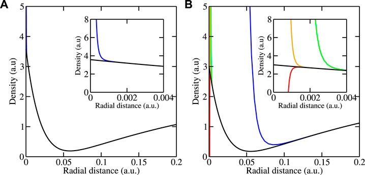
The self-consistent potential determined in this way was used in calculations for the electron density for . In order to save computer resources, a reduced Monkhorst–Pack grid with 6 × 6 × 6 points was applied. Results for the density of the valence electrons near the center of an Ni atom are shown in Figure 2 for and . The insets are blowups on a 100× smaller range. The standard boundary conditions with the recursion relations Eqs 33, 34 lead to the results shown by blue curves. They deviate from the correct behavior below for and below for . These deviations degrade the self-consistency procedure in density-functional calculations unless they are somehow removed by extrapolation, which is cumbersome for large systems, or completely neglected near the atomic centers. Such neglect might be justified for , where the affected volume is a tiny part of the total volume but might be unreasonable for , where the affected volume is non-negligible. Straightforward use of the modified boundary conditions leads to the results shown by green curves. In the left picture, for , the green curve, which is hidden under the black curve, exhibits no divergence at the origin. In the right picture, for , the green curve begins to diverge at , which is considerably smaller than where the blue curve, obtained from the unmodified solutions, begins to diverge. The use of the modified boundary conditions together with one pass through the modified recursion relations (Eqs 49, 50) leads to the orange curves. In the left picture, the orange curve is again hidden under the black curve, while in the right picture, it is considerably better than the green curve by shifting the beginning of the divergence from to . A second pass through the modified recursion relations (Eqs 49, 50) gives only a small improvement seen in the red curve, which begins to diverge at about .

FIGURE 2

The question of whether better results can be obtained by using a larger number of intervals or a higher order of the Chebyshev expansion was investigated by doubling the number of intervals below and by increasing the order to . The results thus obtained are practically identical to those shown in Figure 2. This indicates that the treatment of the auxiliary integral equations with double precision floating-point arithmetic is accurate enough. Whether better results can be obtained by treating the recursion relations more accurately was investigated by using quadruple precision instead of double precision. Then, instead of below , , and , the density results diverge only below , , and . Thus, divergence-free densities as shown by the black curves can be obtained for NiTi at least up to .

4 Summary and outlook

An integral-equation approach was presented for the calculation of irregular solutions of the Schrödinger equation for non-spherical potentials. It was shown how expansions in Chebyshev polynomials can be used to convert the integral equations into systems of algebraic equations, which can be solved by standard software. For that purpose, no explicit construction of the Chebyshev series is needed but only function values at the zeros of the Chebyshev polynomials. It was explained that the numerical effort is considerably reduced by a subinterval technique suggested by Greengard and Rokhlin and that this technique, with appropriately adapted intervals, is beneficial for potentials with a finite number of radial discontinuities; this is because the numerical precision is determined by the smoothness of the potentials between the discontinuities but not by the discontinuous behavior. A numerical investigation was presented for a constant potential and for a realistic non-spherical potential, which was obtained by density-functional calculations for a nickel–titanium alloy. It was shown that accurate bound-state energies can be obtained from the calculated irregular solutions. It was explained how a precise description of the divergent behavior of the coupled irregular solutions can be obtained such that accurate density calculations by complex-contour integrations are possible.

The approach presented can be extended in several directions. It is not restricted to the non-relativistic Schrödinger equation treated here but is also useful for including scalar-relativistic and spin-orbit-coupling effects [22] and for full-relativistic calculations by the Dirac equation (Eq. 23). It can be extended to calculate bound-state energies for non-spherical potentials, although with more effort because of nearby roots caused by degeneracy splitting. It also can be extended to calculate scattering resonances which are determined by zeros of Jost functions in the complex- plane. These zeros can be obtained by contour integrals, for which a Fortran package is available [24]. Calculations of exchange-correlation and Coulomb potentials, which require differentiations and integrations, are easily done with spectral differentiation and integration matrices without introducing additional numerical approximations. An interesting subject for further research is the question of how much numerical precision is needed to evaluate the recursion relations for higher values of beyond , which was the limit set by the present capabilities of the applied KKRnano code.

References

• 1.

  GonzalesRAEisertJKoltrachtINeumannMRawitscherG. Integral equation method for the continuous spectrum radial Schrödinger equation. J Comput Phys (1997) 134:134–49. 10.1006/jcph.1997.5679

  • CrossRef
  • Google Scholar

• 2.

  ClenshawCWCurtisAR. A method for numerical integration on an automatic computer. Numer Math (1960) 2:197–205. 10.1007/bf01386223

  • CrossRef
  • Google Scholar

• 3.

  GreengardL. Spectral integration and two-point boundary value problems. SIAM J Numer Anal (1991) 28:1071–80. 10.1137/0728057

  • CrossRef
  • Google Scholar

• 4.

  GreengardLRokhlinV. On the numerical solution of two-point boundary value problems. Commun Pure Appl Math (1991) 44:419–52. 10.1002/cpa.3160440403

  • CrossRef
  • Google Scholar

• 5.

  HatadaKHayakawaKBenfattoMNatoliCR. Full-potential multiple scattering theory with space-filling cells for bound and continuum states. J Phys Condens Matter (2010) 22:185501. 10.1088/0953-8984/22/18/185501

  • CrossRef
  • Google Scholar

• 6.

  ZellerRDederichsPHÚjfalussyBSzunyoghLWeinbergerP. Theory and convergence properties of the screened Korringa-Kohn-Rostoker method. Phys Rev B (1995) 52:8807–12. 10.1103/physrevb.52.8807

  • CrossRef
  • Google Scholar

• 7.

  ThiessAZellerRBoltenMDederichsPHBlügelS. Massively parallel density functional calculations for thousands of atoms: KKRnano. Phys Rev B (2012) 85:235103. 10.1103/physrevb.85.235103

  • CrossRef
  • Google Scholar

• 8.

  ZellerR. Projection potentials and angular momentum convergence of total energies in the full-potential Korringa-Kohn-Rostoker method. J Phys Condens Matter (2013) 25:105505. 10.1088/0953-8984/25/10/105505

  • CrossRef
  • Google Scholar

• 9.

  ErshovSNVaagenJSZhukovMV. Modified variable phase method for the solution of coupled radial Schrödinger equations. Phys Rev C (2011) 84:064308. 10.1103/physrevc.84.064308

  • CrossRef
  • Google Scholar

• 10.

  ZellerRDeutzJDederichsPH. Application of complex energy integration to selfconsistent electronic structure calculations. Solid State Commun (1982) 44:993–7. 10.1016/0038-1098(82)90320-9

  • CrossRef
  • Google Scholar

• 11.

  KotaniTAkaiH. KKR-ASA method in exact exchange-potential band-structure calculations. Phys Rev B (1996) 54:16502–14. 10.1103/physrevb.54.16502

  • CrossRef
  • Google Scholar

• 12.

  OguraMAkaiH. The full potential Korringa-Kohn-Rostoker method and its application in electric field gradient calculations. J Phys Condens Matter (2005) 17:5741–55. 10.1088/0953-8984/17/37/011

  • CrossRef
  • Google Scholar

• 13.

  RusanuAStocksGMWangYFaulknerJS. Green’s functions in full-potential multiple-scattering theory. Phys Rev B (2011) 84:035102. 10.1103/physrevb.84.035102

  • CrossRef
  • Google Scholar

• 14.

  NewtonRG. Analytic properties of radial wave functions. J Math Phys (1960) 1:452–347. 10.1063/1.1703680

  • CrossRef
  • Google Scholar

• 15.

  RiddersCJF. A new algorithm for computing a single root of a real continuous function. IEEE Trans Circuits Syst (1979) 26:979–80. 10.1109/tcs.1979.1084580

  • CrossRef
  • Google Scholar

• 16.

  AnnabyMHAsharabiRM. Sinc-interpolants in the energy plane for regular solution, Jost function, and its zeros of quantum scattering. J Math Phys (2018) 59:013502. 10.1063/1.5001078

  • CrossRef
  • Google Scholar

• 17.

  VoskoSHWilkLNusairM. Accurate spin-dependent electron liquid correlation energies for local spin density calculations: a critical analysis. Can J Phys (1980) 58:1200–11. 10.1139/p80-159

  • CrossRef
  • Google Scholar

• 18.

  MonkhorstHJPackJD. Special points for Brillouin-zone integrations. Phys Rev B (1976) 13:5188–92. 10.1103/physrevb.13.5188

  • CrossRef
  • Google Scholar

• 19.

  KudohYTokonamiMMiyazakiSOtsukaK. Crystal structure of the martensite in Ti-49.2 at.%Ni alloy analyzed by the single crystal X-ray diffraction method. Acta Mater (1985) 33:2049–56. 10.1016/0001-6160(85)90128-2

  • CrossRef
  • Google Scholar

• 20.

  StefanouNAkaiHZellerR. An efficient numerical method to calculate shape truncation functions for Wigner-Seitz atomic polyhedra. Comp Phys Commun (1990) 60:231–8. 10.1016/0010-4655(90)90009-p

  • CrossRef
  • Google Scholar

• 21.

  ZellerR. Large scale supercell calculations for forces around substitutional defects in NiTi. Phys Status Solidi B (2014) 251:2048–54. 10.1002/pssb.201350406

  • CrossRef
  • Google Scholar

• 22.

  BauerDSGDevelopment of a relativistic full-potential first-principles multiple scattering Green function method applied to complex magnetic textures of nano structures at surfaces. Ph.D. thesis. Aachen, Germany: RWTH Aachen University (2013).

  • Google Scholar

• 23.

  GeilhufeMAchillesSKöbisMAArnoldMMertigIHergertWet alNumerical solution of the relativistic single-site scattering problem for the Coulomb and the Mathieu potential. J Phys Condens Matter (2015) 27:435202. 10.1088/0953-8984/27/43/435202

  • CrossRef
  • Google Scholar

• 24.

  KravanjaPVan BarelMRagosOVrahatisMNZafiropoulosFA. Zeal: a mathematical software package for computing zeros of analytic functions. Comp Phys Commun (2000) 124:212–32. 10.1016/s0010-4655(99)00429-4

  • CrossRef
  • Google Scholar