Multi-quantile systemic financial risk based on a monotone composite quantile regression neural network

This study proposes a novel perspective to calibrate the conditional value at risk (CoVaR) of countries based on the monotone composite quantile regression neural network (MCQRNN). MCQRNN can fix the “quantile crossing” problem, which is more robust in CoVaR estimating. In addition, we extend the MCQRNN method with quantile-on-quantile (QQ), which can avoid the bias in quantile regression. Building on the estimation results, we construct a systemic risk spillover network across countries in the Asia–Pacific region by considering the suffering and overflow effects. A comparison among MCQRNN, QRNN, and MCQRNN-QQ indicates the significance of monotone composite quantiles in modeling CoVaR. Additionally, the network analysis of composite risk spillovers illustrates the advantages of MCQRNN-QQ-CoVaR compared with QRNN-CoVaR. Moreover, the average composite systemic suffering index and the average composite systemic overflow index are introduced as country-specific measures that enable identifying systemically relevant countries during extreme events.

1 Introduction

The Sino–U.S. trade war and the COVID-19 epidemic have caused huge fluctuations in Asia–Pacific stock markets. Compared with other economic organizations, the Asia–Pacific Economic Cooperation (APEC) organization provides a diversified financial markets environment, including developed and developing countries. In addition, APEC’s organizational structure and cooperation mechanism are more flexible, which means member countries cooperate while maintaining autonomy. Moreover, the economic structure of APEC countries is highly complementary; for example, resource-rich countries tend to trade closely with countries with developed manufacturing industries. By establishing interconnectivity, APEC encourages deeper cooperation in infrastructure, trade, and investment among countries in the region. According to statistical data, APEC members account for more than 40% of global trade. Within the region, trade among members is higher than trade with non-members. Despite the large volume of intra-APEC trade, APEC trade relations may depend more on bilateral relationships of large countries such as China and the United States than other economic organizations such as the European Union. This means that the trade closeness of APEC is greatly affected by the policy changes of large countries. Consequently, in the stage of Sino–U.S. trade friction, the trade cooperation of member countries will undergo great changes.

In the COVID-19 phase, the economic conditions of China and the United States will directly affect the risk level of the organization’s members. Therefore, the research on systemic financial risks among APEC member countries in this paper is helpful for a deeper analysis of the risk contagion mechanisms between different economies and could provide a supplement to existing literature. Growing uncertainty results in countries facing cross-border risk shocks, making the issue of systemic risk a renewed focus of research by academics and regulators. Systemic risk caused by the bankruptcy of systemically important economies is primarily the failure of the financial system. From the aspect of international markets, when an important node is damaged by a shock, other markets may also be affected and could eventually be contagious to the entire financial system.

To measure the systemic risk, studies in recent years have begun to focus on the risk contagion or spillover effect [1]. The former is mainly from a theoretical modeling perspective [2–6]. Additionally, more focus on empirical measurement provides compositions for the “edge” of the financial network. For instance, Engle (2002) constructs the GARCH-DCC method to capture the risk spillover among market indexes [7]. Rodriguez (2007) measures the interdependence among East Asian stock via switching-parameter copulas [8]. Billio et al. (2012) prompt the empirical framework of a risk spillover network based on Granger causality [9]. Diebold and Yılmaz (2014) involve variance decomposition in risk spillover and analyze the vulnerability by financial networks [10]. Baruník and Křehlík (2018) study the risk spillover from aspects of heterogeneous frequency responses to shock [11].

The risk modeling system of this paper is an addition to the conditional value at risk ($CoVaR$), which is the systemic risk approach [12]. Adrian and Brunnermeier (2016) define $∆CoVaR$ as the change of system’s value at risk in the condition of one single institution’s loss, which has provided a new perspective for risk spillover effects [12]. Nevertheless, the original $CoVaR$ needs to assume a linear relationship between the return of market indexes and institutions’ stock prices. Thus, Hautsch et al. (2015) provide a paradigm of multivariate $CoVaR$, which is based on the marginal effect of risk spillovers among financial institutions [13]. Furthermore, based on $SIM-CoVaR$, Fan et al.(2018), Härdle et al. (2016) propose a tail event driven network technique ($TENET$), where the $∆CoVaR$ is replaced as the partial differentiation of multivariate nonlinear $CoVaR$ [14, 15]. On this basis, Keilbar and Wang (2022) adapt the $TENET$ model approach based on a neural network method, which also uses partial differential to calculate the marginal effect among agents [16]. $QRNN-CoVaR$ has already been employed for risk spillover among inter-industries and energy markets [17, 18]. Moreover, graph learning in attributed networks are used in risk spillover by different node-to-cluster distance functions [19, 20].

This paper seeks to expand the research perspective on systemic financial risk by examining the composite risk spillover effects among financial markets to avoid possible errors in the setting of quantiles. We construct the composite risk spillover measure based on the multi-quantile $CoVaR$ by multi-quantile $CAViaR$ ($MQ-CAViaR$) and quantile-on-quantile regression ($QQR$). $QQR$ has been widely involved in correlation and spillover effect [21–23], although it has not been adopted by $CoVaR$ estimation. It is found that the concept of $QQR$ is suitable for systemic financial risk because there are two-sided quantile sets in the $CoVaR$ definition. However, in traditional methodology, both the stand-alone quantiles and exposed quantiles are set as a fixed small number (normally 5%). If $CoVaR$ is extended to multiple (stand-alone) quantiles, a tough problem, “quantile crossing,” will emerge and raise a paradox of “higher risk but less¹ loss” [24, 25]. The problem of non-monotonicity of risk indicators arises when estimating CoVaR using single-quantile regression. However, financial risk indicators must ensure their monotonicity, so the issue of quantile crossover must be addressed [26, 27].

Some studies focus on this problem. Acharya et al. (2017) assessed the expected loss below one quantile in dealing with the problem of quantile crossing [27]. Catania and Luati (2023) used a semiparametric model to satisfy the condition of non-crossing quantiles [28]. By investigating the $QQ-CoVaR$, this paper not only obtains a more robust risk spillover measure, but also facilitates the examination of the characteristics of nonlinear systemic risks in each market. In addition, although some studies have addressed the risk-related networks of financial markets in the Asia–Pacific region [29–31], few visualize the systemic risk of quantile regression neural networks. The findings of this paper should make an important contribution to the field of capturing systemic risk spillovers among financial markets and recognition of risk sources.

This paper proposes a quantile-on-quantile regression to examine the two-sided quantile in CoVaR estimation. The effects of systemic risk are analyzed by three-dimensional surface plots in empirical research. We extend the quantile regression in the systemic risk approach with a monotone composite quantile regression neural network, which can not only be suitable for solving the nonlinear issue but also optimize the “quantile crossing” problem. Moreover, we introduce the composite systemic suffering indicator, the composite systemic overflow indicator, and the total composite overflow indicator as three country-specific measures to identify systemically relevant countries in the Asia–Pacific region during extreme events.

This article makes three main contributions. First, we estimate the systemic financial risk through a new perspective that adopts 3D surface plots. Second, multi-quantiles are adopted in the model to capture the multi-state characteristics of risk. Third, MCQRNN is used to relieve the quantile crossing problem.

The remainder of the paper will be organized as follows: Section 2 will (i) introduce the multi-quantile $CoVaR$ based on monotone composite neural network quantile regression ($MCQRNN$) and (ii) describe the methodology of $MCQRNN-QQ-CoVaR$ in details. After constituting the risk modeling system step by step, the empirical results based on Asia–Pacific stock markets and discussion will be presented in Section 3. Finally, a conclusion of this paper and suggestions for future study are drawn in Section 4.

2 Materials and methods

2.1 The monotone composite neural network of quantile regression ($\mathit{M}\mathit{C}\mathit{Q}\mathit{R}\mathit{N}\mathit{N}$) method

A quantile regression model based on a linear regression equation estimates parameters for $\tau$ quantiles under the variable $Y_t$ by introducing an indicative function in the loss function [32], defined as Equation 1.

$\underset{\beta }{\min }{\displaystyle \sum _{t=1}^n}{\rho }_{\tau }\left(Y_t-X_t\beta \right),(1)$

where ${\rho }_{\tau }\left(z\right)=\left|z\right|\cdot \left|\tau -I\left(z<0\right)\right|$ is the loss function at the quantile level of $\tau$ (known as the pinball loss function). Where $I\left(z<0\right)$ is the indicative function, the value is $1$ when the independent variable $z<0$; otherwise, the value is $0$. However, this model only considers linear relationships between the variables, which cannot state the effect of non-linearity. For this reason, Taylor (2000) involved a neural network model called the quantile regression neural network approach ($QRNN$) [33]. Cannon (2018) extended the $QRNN$ to the monotone composite neural network of quantile regression ($MCQRNN$), which can mitigate the “quantile crossing” problem [34]. The comprehensive estimations of multi-quantile $CoVaR$ can be obtained by adjusted $MCQRNN$. Assuming the number of market indexes is $N$ and their price returns are $\left\{R_t^i\right\}$, the conditional value at risk of market $i$ in level of quantile $q_s$ can be obtained by $h^i\left(R_t^{-i},q_s\right)$ defined as² Equation 2.

$h^i\left(R_t^{-i},q_s\right)\equiv {\displaystyle \sum _{m=1}^{M_n}}\left[{\omega }_m^i\cdot \psi \left(e^{{\omega }_m^{ii}}\cdot q_s+{\displaystyle \sum _{j\ne i}}{\omega }_m^{ji}{R}_t^j+b_m^i\right)\right]+b^i(2)$

The difference between $QRNN$ and $MCQRNN$ is introducing quantile $q_s$ as an input variable with a positive weight of $e^{{\omega }_m^{ii}}$. In addition, the nonlinear activation function $\psi \left(\cdot \right)$ is assumed to be invariant and known. The parameter of each node $m$ in the hidden layer consists of weights $\left\{{\omega }_m^{ji}\left|\left.j\ne i\right\}\right.\right.$ and the intercept $b_m^i$, while the output layer parameters are ${\omega }_m^i$ and $b^i$. These parameters are verified to be consistent and asymptotically normal under large sample and regularity conditions. Moreover, they converge to the true function at a certain rate [35, 36].

However, the loss function in the quantile regression is not differentiable everywhere. It limits the use of artificial neural networks’ regular algorithms (ANNs) in $MCQRNN$. Therefore, it is necessary to adjust the form of the loss function. One approach is to add a Huber norm $h\left(u\right)$ [37], which allows a smoothing approximation to the error term near the origin. Furthermore, $h\left(u\right)$ is a hybrid $L^1/L^2-norm$, which makes it possible to use standard gradient-based optimization algorithms.

In addition, when the capacity of the neural network is large, it is prone to over-fitting problems. Choosing a modest neural network structure and hyperparameters is an effective approach often used in machine learning. In a single hidden layer network, the most important hyperparameter is the number of hidden nodes $M_n$. Therefore, choosing the appropriate number of nodes can reduce the capacity of the neural network and avoid the over-fitting phenomenon. In addition, Bishop (1995) proposed alleviating this problem by introducing weight decay regularization [38]. Such regularization requires adding an additional penalty term to the weight parameter ${\omega }_{k,m}^h$. Referring to model of Cannon [39, 40], the final estimator is set as Equation 3 included a quadratic penalty term.

$\underset{{\mathrm{h}}^{\mathrm{i}}}{\min }\frac{1}{\text{TS}}{\displaystyle \sum _{\mathrm{t}=1}^{\mathrm{T}}}{\displaystyle \sum _{\mathrm{s}=1}^{\mathrm{S}}}\mathrm{\rho }{{\displaystyle \sum _{\mathrm{t}=1}^{\mathrm{T}}}}_{{\displaystyle \sum _{\mathrm{s}=1}^{\mathrm{S}}}}^{\mathrm{\rho }}\left({\mathrm{R}}_{\mathrm{t}}^{\mathrm{i}}-{\mathrm{h}}^{\mathrm{i}}\left({\mathrm{R}}_{\mathrm{t}}^{-\mathrm{i}},{\mathrm{q}}_{\mathrm{s}}\right)\right)+\frac{\mathrm{\lambda }}{{\mathrm{M}}_{\mathrm{n}}}{\displaystyle \sum _{\mathrm{m}=1}^{{\mathrm{M}}_{\mathrm{n}}}}{\left({\mathrm{\omega }}_{\mathrm{m}}^{\mathrm{i}}\right)}^2+\frac{\mathrm{\lambda }}{{\mathrm{M}}_{\mathrm{n}}\mathrm{N}}{\displaystyle \sum _{\mathrm{m}=1}^{{\mathrm{M}}_{\mathrm{n}}}}{\left({\mathrm{e}}^{{\mathrm{\omega }}_{\mathrm{m}}^{\text{ii}}}\right)}^2+\frac{\mathrm{\lambda }}{{\mathrm{M}}_{\mathrm{n}}\mathrm{N}}{\displaystyle \sum _{\mathrm{m}=1}^{{\mathrm{M}}_{\mathrm{n}}}}{\displaystyle \sum _{\mathrm{j}\ne \mathrm{i}}}{\left({\mathrm{\omega }}_{\mathrm{m}}^{\text{ji}}\right)}^2,(3)$

where $\lambda$ is the parameter that regulates the weight of the quadratic penalty term in the loss function. When $\lambda$ is $0$, this regression is transformed to an ordinary $MCQRNN$. In this paper, simple sampling is used to train neural networks. According to the experience of [40] and [16], we selected 50% of the samples from the sample period as the training set to train the loss function, which is Equation 3, in the MCQRNN model. Except for $\lambda$ and $M_n$ hyperparameters, the intercept and weights of the neural network are trained. Otherwise, too large $\lambda$ will lead to the loss of non-linear characteristics of the model, when the transfer function $\psi$ is the sigmoidal hidden layer transfer function, such as hyperbolic tangent $\mathit{tanh}$. To balance the degree of the over-fitting and the prediction accuracy, $\lambda$ is set to equal to $2$ here. Furthermore, the optimization of the loss function as shown in Equation 3 can be achieved by using a quasi-Newton optimization algorithm, which is less complex and more appropriate for the computational complexity in this paper. The quantile regression neural network process is visualized in Figure 1.

Figure 1

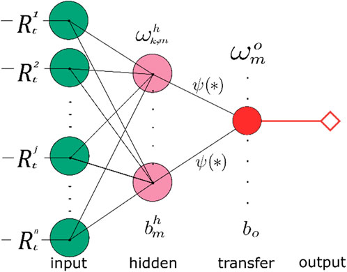
Figure 1. Quantile regression neural network process.

2.2 Calibrate systemic risk system

The calibration details of $MCQRNN-QQ-CoVaR$ are explained in this section. There are four steps involved in the systemic risk system calibration. The first step is the estimation of $VaR$ based on $CAViaR$. Next, the results are used to estimate $CoVaR$ with $MCQRNN$ and $QQ$ for each country. In the third step, the composite risk spillover effects are calculated by resulting in an extreme risk spillover measure. Finally, the systemic risk measures are proposed based on the systemic risk network. The process of the risk modeling system is demonstrated in Figure 2 as follows:

Step 1: Estimation of value at risk with $CAViaR$

Figure 2

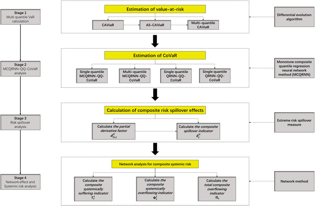
Figure 2. Flowchart of the risk modeling systems.

Because it is challenging to select common macro-state variables for all indexes, the linear quantile regression of value at risk is no longer suitable for measuring the tail risk of stock markets. Hence, $CAViaR$ is adopted in the first step [41]. Given the asymmetric effects of the rise and fall of each index, $AS-CAViaR$ at the quantile level of $p_l$ can be estimated in the following Equation 4 [42]³:

$CAVia{R}_{l,t}^j\left(\mathrm{\beta }\right)={\beta }_1+{\beta }_{2}CAVia{R}_{l,t-1}^j\left(\mathrm{\beta }\right)+{\beta }_3{\left[R_{t-1}^j\right]}^{+}+{\beta }_4{\left[R_{t-1}^j\right]}^{-},(4)$

where ${\left[R_{t-1}^j\right]}^{+}$ is the absolute value of market index $j$’s return when the lagged log-return is larger than zero, and the rest is $0$. $R_{t-1}^{j-}$ is the absolute value when the lagged log-return is minus zero. $\beta =\left[{\beta }_1,{\beta }_2,{\beta }_3,{\beta }_4\right]$ is the vector of the parameters. By utilizing the differential evolution algorithm [43] and the loss function similar to Equation 1, the ${CAViaR}_{l,t}^j$ is an appropriate risk indicator for individual stock market $j$ at the quantile level of $p_l$.

Step 2: Estimation of $CoVaR$ with $MCQRNN-QQ$

First, the $MCQRNN$ method is adopted to estimate ${\widehat{\mathit{h}}}^{\mathit{i}}\left({\mathit{R}}_{\mathit{t}}^{-\mathit{i}},{\mathit{q}}_{\mathit{s}}\right)$ based on Equation 3. Additionally, given the quantiles of stand-alone $\left[q_1,q_2,...,q_S\right]$ and quantiles of exposed risk $\left[p_1,p_2,...,p_L\right]$, the quantile-on-quantile conditional value at risk ($QQ-CoVaR$) can be obtained by the $MCQRNN$. $QQ-CoVaR$ [16] is estimated similar to $CoVaR$ [12] and $TENET$ [44]. To embed the dependency among financial markets, the estimation of $CoVaR$ by $MCQRNN$ is introduced. Following [16], the definition of $CoVaR$ is adjusted as Equation 5 to adapt to a multivariate model.

$Prob\left(R_t^i<CoVa{R}_{l,t}^{s,i}|R_t^j=CAVia{R}_{l,t}^j,\forall j\ne i\right)=q_s.(5)$

Assume the $CoVaR$ of market index $i$ is predictable via function $h^i\left(R_t^{-i},q_s\right)$, and other indexes’ current return $\left\{{\left.R_t^j\right\}}_{j\ne i}\right.$, ${\widehat{h}}^i$ is the estimator of the function and can be trained by the $MCQRNN$ algorithm [34]. Therefore, the $CoVaR$ in the condition of each risk state ($p_l,q_s$) can be obtained by Equation 6.

$CoVa{R}_{l,t}^{s,i}=h^i\left({CAViaR}_{l,t}^{-i},q_s\right).(6)$

It should be noted that, in distinction to Keilbar and Wang, this paper estimates $CoVa{R}_{l,t}^{s,i}$ for all quantiles of the whole range⁴. Thus, the $CoVaR$ of each market index $i$ can be expressed as a three-dimensional surface at each time point by setting the $X$ and $Y$ axes to denote different quantile levels $p$ and $q$, respectively. The z-axis values are $CoVa{R}_{l,t}^{s,i}$. There is an advantage of reflecting both the non-linear relationship between $CoVa{R}_{l,t}^{s,i}$ varying with the risk condition $\left\{{CAViaR}_{l,t}^j\right\}$ and the $CoVaR$ at each of its own risk levels $q$.

Step 3: Calculation of composite risk spillover effects

To examine the margin impact of index $j$ on the $CoVa{R}_{l,t}^{s,i}$, the partial derivative is taken, which is named $d_{ls,t}^{ji}$. According to the format of the function ${\widehat{h}}^i$ estimated by $MCQRNN$, the risk spillover from $j$ to $i$ is expressed as Equation 7,

${\mathit{d}}_{\mathit{ls},\mathit{t}}^{\mathit{j}\mathit{i}}=\frac{\partial \widehat{h}\mathit{i}}{\partial {\mathit{R}}_{\mathit{t}}^{\mathit{j}}}\left(\mathit{CAVia}{\mathit{R}}_{\mathit{l},\mathit{t}}^{-\mathit{i}},{\mathit{q}}_{\mathit{s}}\right)={\displaystyle \sum _{\mathit{m}=1}^{{\mathit{M}}_{\mathit{n}}}}\left[{\widehat{\omega }}_{\mathit{m}}^{\mathit{i}}{\widehat{\omega }}_{\mathit{m}}^{\mathit{ji}}\cdot {\mathit{\psi }}^{\prime }\left({\mathit{e}}^{{\widehat{\omega }}_{\mathit{m}}^{\mathit{ii}}}\cdot {\mathit{q}}_{\mathit{s}}+{\displaystyle \sum _{\mathit{j}\ne \mathit{i}}}{\widehat{\omega }}_{\mathit{m}}^{\mathit{ji}}\mathit{CAVia}{\mathit{R}}_{\mathit{l},\mathit{t}}^{\mathit{j}}+{\widehat{b}}_{\mathit{m}}^{\mathit{i}}\right)\right],(7)$

where the derivative of the transfer function is set as ${\psi }^{\prime }=\frac{1}{2}\left(1-{\tanh }^2\left(\frac{z}{2}\right)\right)$, and all parameters are trained by $MCQRNN$. This measure should be based on the accuracy of the $CoVaR$ estimation, but the $QRNN$, as a non-linear neural network model, is prone to over-fitting at a single quantile. Consequently, the $MCQRNN$ adopted in this paper is able to reduce the impact of potential fitting error at a single quantile on the overall risk spillover. Considering the risk spillovers at different quantiles, the composite risk spillover can be defined as ${\delta }_t^{ji}$ as Equation 8.

${\delta }_t^{ji}=\left\{\begin{array}{l}\frac{1}{SL}{\displaystyle \sum _{s=1}^S}{\displaystyle \sum _{l=1}^L}\left[\left.\left(1+\left|CAVia\right.R_{l,t}^j\left|)\cdot \left(1+\right|\right.CoVa{R}_{l,t}^{s,i}\left|)\cdot \right|d_{ls,t}^{ji}\right.\right|\right],ifj\ne i\\ 0, ifj=i,\end{array}\right.(8)$

where the $\left|d_{ls,t}^{ji}\right|$ is the absolute value of risk spillover, and the risk-weighted composite risk spillover from index $j$ to $i$ is defined as ${\delta }_t^{ji}$. Because the absolute value of the risk indicators ($CAViaR$, $CoVaR$) in the more extreme state is larger, the risk spillover in the extreme risk state couple $\left(p_l,q_s\right)$ accounts for more weight in the aggregate indicator.

To reflect the sensitivity of average-level composite risk spillover to the two-sided quantiles, we decompose the ${\overline{\delta }}^{ji}={\sum }_{t=1}^T{\delta }_t^{ji}$ into two partial spillover indicators ${\delta }_s^{ji}$ and ${\delta }_l^{ji}$, as Equation 9.

$\begin{array}{c}{\overline{\delta }}_s^{ji}=\left\{\begin{array}{ll}\frac{1}{TS}{\displaystyle \sum _{t=1}^T}{\displaystyle \sum _{l=1}^L}\left[\left(1+\left|CAVia{R}_{l,t}^j\right|\right)\cdot \left(1+\left|CoVa{R}_{l,t}^{s,i}\right|\right)\cdot \left|d_{ls,t}^{ji}\right|\right],& if j\ne i\\ 0,\hfill & if j=i\end{array}\right.\\ {\overline{\delta }}_l^{ji}=\left\{\begin{array}{ll}\frac{1}{TS}{\displaystyle \sum _{t=1}^T}{\displaystyle \sum _{s=1}^S}\left[\left(1+\left|CAVia{R}_{l,t}^j\right|\right)\cdot \left(1+\left|CoVa{R}_{l,t}^{s,i}\right|\right)\cdot \left|d_{ls,t}^{ji}\right|\right],& if j\ne i\\ 0,\hfill & if j=i\end{array}\right.\end{array}(9)$

The partial spillover indicators are used to reflect the average impact of the two-sided risk state on the spillover from market $j$ to market $i$ in the sample period. The partial spillover indicator of $p_l$ side ${\delta }_l^{ji}$ is the composite spillover effect at the exposed risk state of $p_l$, which reflects the sensitivity to the risk state of the entire system. Correspondingly, the ${\delta }_s^{ji}$ indicates the response of spillover effect to the change in stand-alone risk status $q_s$. In addition, it is necessary to consider the spillover of market $j$ to $i$ under the most extreme conditions, that is, $q_1$ or $p_1$. Hence, we consider the conditional partial spillover indicators under the fixed $q_1$ quantile or fixed $p_1$ as Equation 10.

$\begin{array}{c}\left.{\overline{\delta }}_{1s}^{ji}=\frac{1}{T}\left.{\displaystyle \sum _{t=1}^T}\right|d_{1s,t}^{ji}\right|\text{and}\left.{\overline{\delta }}_{l1}^{ji}=\frac{1}{T}\left.{\displaystyle \sum _{t=1}^T}\right|d_{l1,t}^{ji}\right|\end{array}.(10)$

The non-linear characteristics of inter-market risk spillover can be analyzed by comparing the two types of partial spillover indices under different quantiles, and the mutation quantile of spillover can be captured. In addition, to reflect the extreme risk spillover, the ${\overline{\delta }}_{11}^{ji}={\displaystyle \sum _t^T}{d}_{11,t}^{ji}$ is defined as spillover at a single quantile. If this indicator is calculated by $QRNN$, it will be the same as the spillover defined by [18].

Last but not least, similar to the partial spillover indicators, four partial $CoVaR$ terms can be defined as the average $CoVaR$ when the one-side quantile takes different values under the condition of the other fixed, that is, ${\overline{CoVaR}}_s^i$ and ${\overline{CoVaR}}_l^i$. To reflect the tail risk in the extreme condition, the traditional $CoVaR$ estimated by $QRNN$ and $MCQRNN$ are also calculated as ${\overline{CoVaR}}_{1s}^i$, ${\overline{CoVaR}}_{l1}^i$. Taking the ${\overline{CoVaR}}_s^i$ and ${\overline{CoVaR}}_{1s}^i$ as an example, Equation 11 is consistent with the partial spillover ${\overline{\delta }}_s^{ji}$.

$\left\{\begin{array}{c}{\overline{CoVaR}}_s^i=\frac{1}{TL}{\displaystyle \sum _{l=1}^L}{\displaystyle \sum _{t=1}^T}CoVa{R}_{l,t}^{s,i}\\ {\overline{CoVaR}}_{1s}^i=\frac{1}{T}{\displaystyle \sum _{t=1}^T}CoVa{R}_{l,t}^{s,i}{|}_{l=1}.\end{array}\right.(11)$

The quantile crossing problem in the estimation of $CoVaR$ can be described and counted as Equation 12,

$\left.\exists s_1<s_2\left.,\right|{\overline{CoVaR}}_{s_1}^i\left|<\right|{\overline{CoVaR}}_{s_2}^i\right|.(12)$

For each market, the total number of “quantile crossing” problems can be accumulated by a monotonicity test. Because the $CoVa{R}_t$ is more adaptable in financial markets, we employ $CoVa{R}_{1,t}^{s,i}$, ${\overline{CoVaR}}_{1s}^i$, and ${\overline{CoVaR}}_s^i$ to accumulate numbers of “quantile crossings” for each market.

Step 4: Network analysis for composite systemic risk

The average measures of composite systemic risk will be gained in the final step. First, because the risk spillover of market index $j$ on market index $i$ involves two quantiles $p_l$ and $q_s$, the average indicators are composited and averaged. Referring to previous works [16, 45], the composite systemic suffering indicator ${\mathrm{\Gamma }}_t^i$ should be aggregated as Equation 13. The composite index is weighted by the own risk of each spillover emitter. This is because if market $j$ has higher own risks, market $i$ will bear more systemic risk spillover.

${\mathrm{\Gamma }}_t^i=\frac{1}{SL}{\displaystyle \sum _{s=1}^S}{\displaystyle \sum _{l=1}^L}{\displaystyle \sum _{j\ne i}}\left[\left(1+\left|CAVia{R}_{l,t}^j\right|\right)\cdot \left|d_{ls,t}^{ji}\right|\right].(13)$

Second, the composite systemic overflow indicator ${\mathit{\Phi }}_t^j$ can be defined as Equation 14.

${\mathit{\Phi }}_t^j=\frac{1}{SL}{\displaystyle \sum _{s=1}^S}{\displaystyle \sum _{l=1}^L}{\displaystyle \sum _{i\ne j}}\left[\left(1+\left|CoVa{R}_{l,t}^{s,i}\right|\right)\cdot \left|d_{ls,t}^{ji}\right|\right].(14)$

To reveal the trend of the spillover effect, the total composite overflow indicator ${\mathrm{\Pi }}_t$ can be calculated as Equation 15.

${\mathrm{\Pi }}_t=\frac{1}{SL}{\displaystyle \sum _{s=1}^S}{\displaystyle \sum _{l=1}^L}{\displaystyle \sum _{j=1}^N}{\displaystyle \sum _{i\ne j}}\left[\left(1+\left|CAVia{R}_{l,t}^j\right|\right)\cdot \left(1+\left|CoVa{R}_{l,t}^{s,i}\right|\right)\cdot \left|d_{ls,t}^{ji}\right|\right](15)$

The total overflow indicator can be regarded as the weighted sum of ${\mathit{\Phi }}_t^j$, which reflects the changing trend of risk spillover time of each market in the sample.

Lastly, the adjusted adjacency matrix is defined as Equation 16.

$A_t=\left\{\begin{array}{cccc}0& {\overline{\delta }}_t^{12}& \cdots & {\overline{\delta }}_t^{1N}\\ {\overline{\delta }}_t^{21}& 0& \cdots & {\overline{\delta }}_t^{2N}\\ ⋮& \cdots & \ddots & ⋮\\ {\overline{\delta }}_t^{N1}& {\overline{\delta }}_t^{N2}& \cdots & 0\end{array}\right\}.(16)$

The adjusted adjacency matrix accounts are the risk spillover indicators. Systemic spillover effects are thus determined by the marginal effects of the $MCQRNN$ procedure, as well as by the $VaR$ and $CoVaR$ of the considered countries.

3 Results and discussion

3.1 Data and descriptions

We select the stock market indices of $N=18$ representative countries or regions from the Asia–Pacific Economic Cooperation (APEC) organization varying from January 2012 to December 2021 as sample data. Due to the weekday effect and excessive short-term volatility noise in daily frequency data, the daily returns of stock indexes taken from the WIND database are transformed into weekly data. The logarithmic return is calculated using the closing price on the last trading day of each week. Adopting weekly frequency data can effectively avoid the problem of time differences between the markets, and the data for each week can simply be treated as contemporaneous. The indexes and their abbreviations of regions for the 18 markets are shown in Table 1.

Table 1

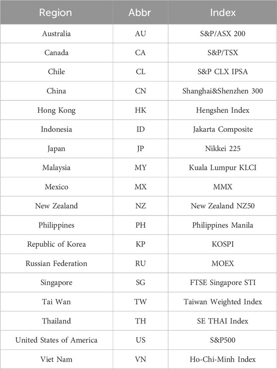
Table 1. Abbreviations of regions and indexes.

As shown in Table 2, the total number of observations is 9,396 because some markets have missing samples due to the holidays or other factors. The average weekly return of each market is all positive, which indicates that the indices prices of Asia–Pacific stock markets at the end of 2021 are higher than they were in 2011. It is worth noting that the minimum value of all samples is −20.13%, which is the weekly return of the Chile index in the fourth week of March 2020. The maximum value occurred in the next week, which is 15.81% in Japan. The World Health Organization recognized the COVID-19 outbreak as a global pandemic on 11 March 2020. After 2 weeks of declines, most global stock markets rebounded sharply in the last week of March. Except for the stock markets of Mexico, mainland China, and Hong Kong, all the financial markets have a kurtosis of 3 or more in their return distributions. The return curves show a sharp peak pattern, which indicates that the outliers are more dispersed. In addition, the skewness of all the markets in the sample is negative, indicating that the return series of each market is left skewness; that is, the probability of negative extreme value is higher than positive. The augmented Dickey–Fuller (ADF) value of each market return is negative and less than the test critical value at the 1% significant level, rejecting the null hypothesis of a unit root. All Jarque–Bera (JB) statistics are significant at the 1% level, which rejects the null hypothesis of Gaussian distribution for the market returns.

Table 2

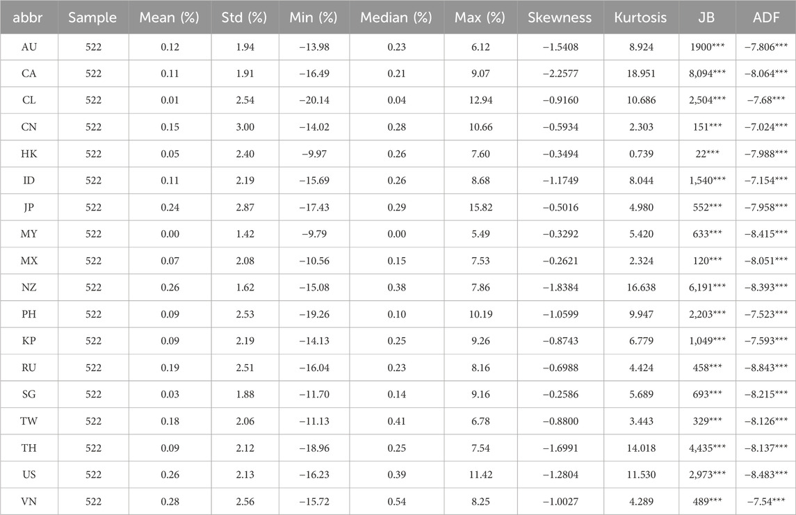
Table 2. Descriptive statistics.

3.2 Estimation of multi-quantile $\mathit{C}\mathit{A}\mathit{V}\mathit{i}\mathit{a}\mathit{R}$ and $\mathit{C}\mathit{o}\mathit{V}\mathit{a}\mathit{R}$

3.2.1 Estimation of multi-quantile $\mathit{C}\mathit{A}\mathit{V}\mathit{i}\mathit{a}\mathit{R}$

The $CAViaR$ series for each market return can be calculated based on the methodology described in Section 2.2. Different from the conventional $VaR$ calculation, a list of quantiles [5%, 10%, , 95%] is selected to calculate the multi-quantile $CAViaR$ ($MQ-CAViaR$) at each quantile.

The $MQ-CAViaR$ line diagrams of the United States and China are shown in Figure 3⁵. Scatter points in gray represent the weekly returns, while the line represents the $CAViaR$ at each quantile level. As can be seen from the diagrams, the $MQ-CAViaR$ lines approximately envelop the points of return. From the perspective of the whole-time sequence, the Chinese stock market fluctuates more. In contrast, the US stock market returns are more concentrated overall, except for two extreme values: late 2011 and early 2020. Since the second half of 2011, the US stock market has suffered severe shocks, especially due to the downgrade of the US credit rating and the continued deterioration of the European debt crisis, which triggered investor panic and increased US stock volatility. In addition, 2020 was the time of the worldwide outbreak of the COVID-19 pandemic. These two unexpected events hugely impacted the US stock market, while during the remaining time, the US stock market was relatively stable compared to the Chinese stock market. The patterns of the $CAViaR$ charts reflect the differences in the maturity of the two markets. In terms of general trends, the Chinese stock market is more volatile, with larger absolute market returns under extreme conditions because of the frequent policy intervention and excessive proportion of individual investors. Meanwhile, the $CAViaR$ of the US market is smaller in absolute terms, indicating that its market is able to return to a steady state relatively quickly after a short-term shock. Furthermore, the $CAViaR$ lines of China at different quantiles are asymmetrical in the vertical dimension. Its envelope area is larger below the zero value; in other words, its value stays more in the negative zone. In contrast, the $CAViaR$ values of the United States are more concentrated in the positive zone. According to the distribution of returns, the Chinese stock market tends to suffer losses, while the US stock market tends to make profits.

Figure 3

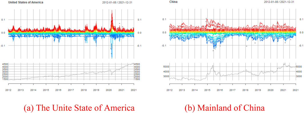
Figure 3. Multi-quantile CAViaR diagrams of the United States and China. (A) The United States of America and (B) mainland China.

3.2.2 Comparison of $\mathit{C}\mathit{o}\mathit{V}\mathit{a}\mathit{R}$ estimated by $\mathit{Q}\mathit{R}\mathit{N}\mathit{N}$ and $\mathit{M}\mathit{C}\mathit{Q}\mathit{R}\mathit{N}\mathit{N}$

According to the count method described in Equation 11, the number of cross-quantile occurrences in each market is shown in Table 3. Because 18 pairs of adjacent quantiles and 522 periods in each market are compared, the first column of the table shows that the quantile crossing is a common problem in the estimation of ${CoVaR}_{1,t}^{s,i}$. Even when considering the average level, the quantile crossing is still obvious when comparing 18 pairs of quantiles. However, $MCQRNN$ completely eliminates this problem. To further analyze the level of risk in the market under different conditions, as described in Section 2.2, the three-dimensional mesh-surface graphs were plotted to present the $QQ-CoVaR$ at each $q_s$ quantile of a stand-alone state and $p_l$ quantile of an exposed state. Figure 4 presents the MCQRNN-QQ-CoVaR plots for other markets indexes⁶.

Table 3

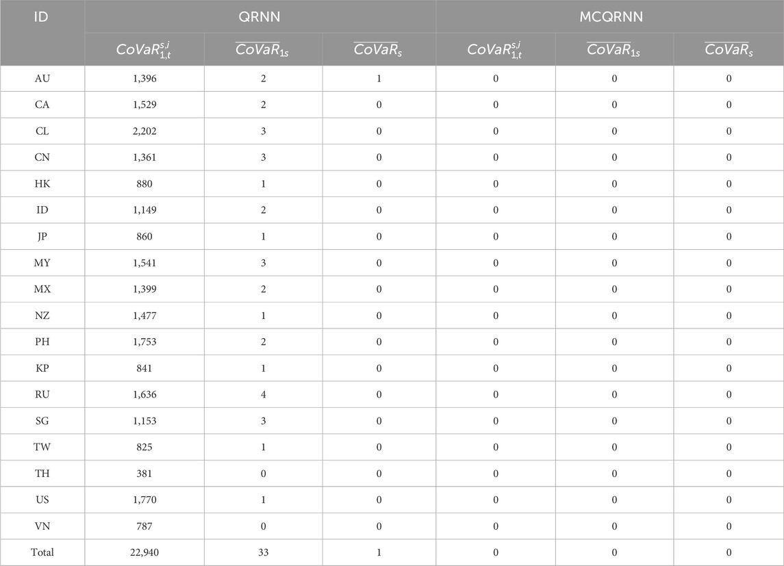
Table 3. Cross-quantile count by the monotonicity test.

Figure 4

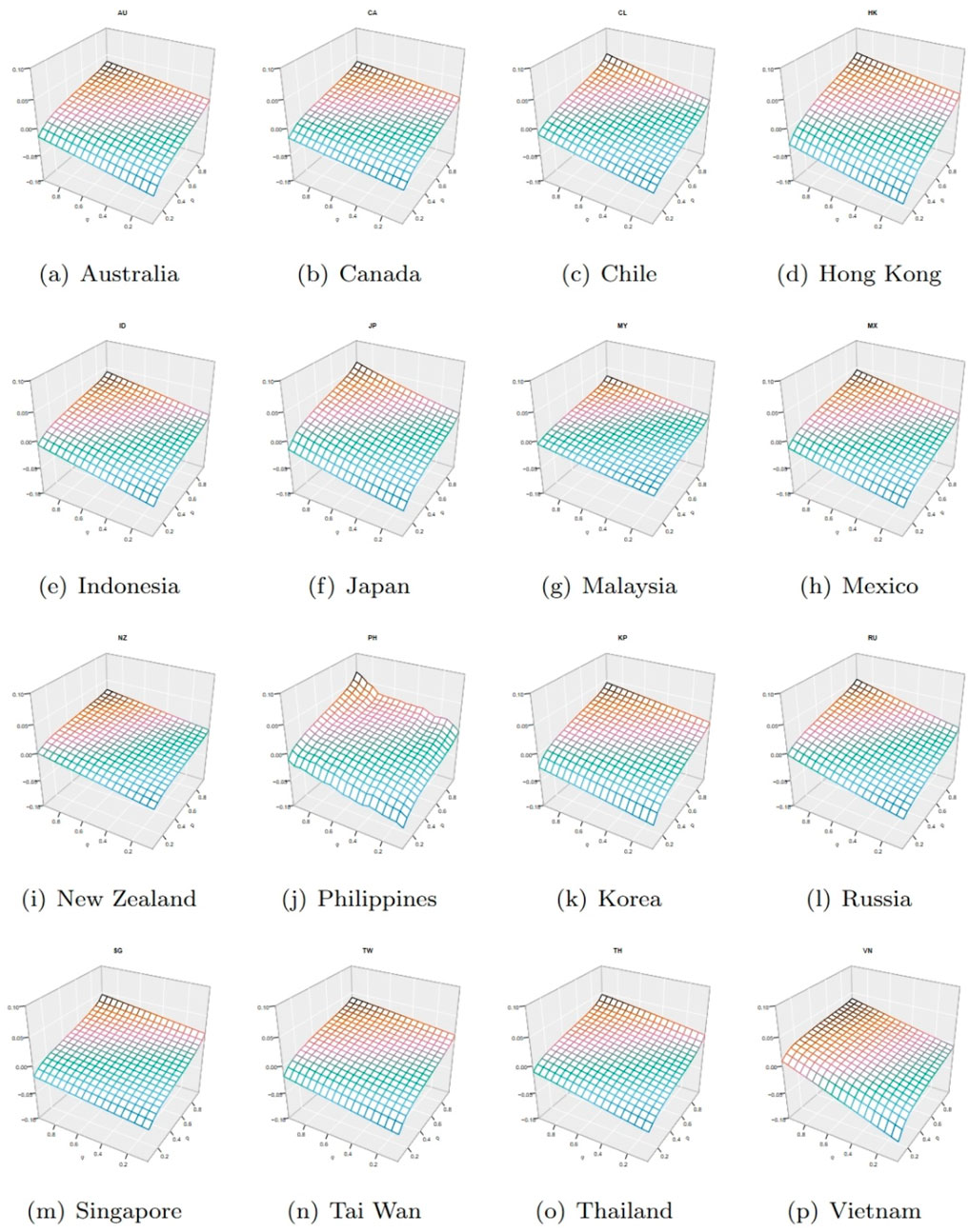
Figure 4. MCQRNN-QQ-CoVaR 3D-surface plots for other market indexes. (A) Australia, (B) Canada, (C) Chile, (D) Hong Kong, (E) Indonesia, (F) Japan, (G) Malaysia, (H) Mexico, (I) New Zealand, (J) Philippines, (K) Korea, (L) Russia, (M) Singapore, (N) Tai Wan, (O) Thailand, and (P) Vietnam.

We select China and the United States as outstanding examples. Figure 5 represents the level of $CoVaR$ and non-linear characteristics in the United States and mainland China⁷.

Figure 5

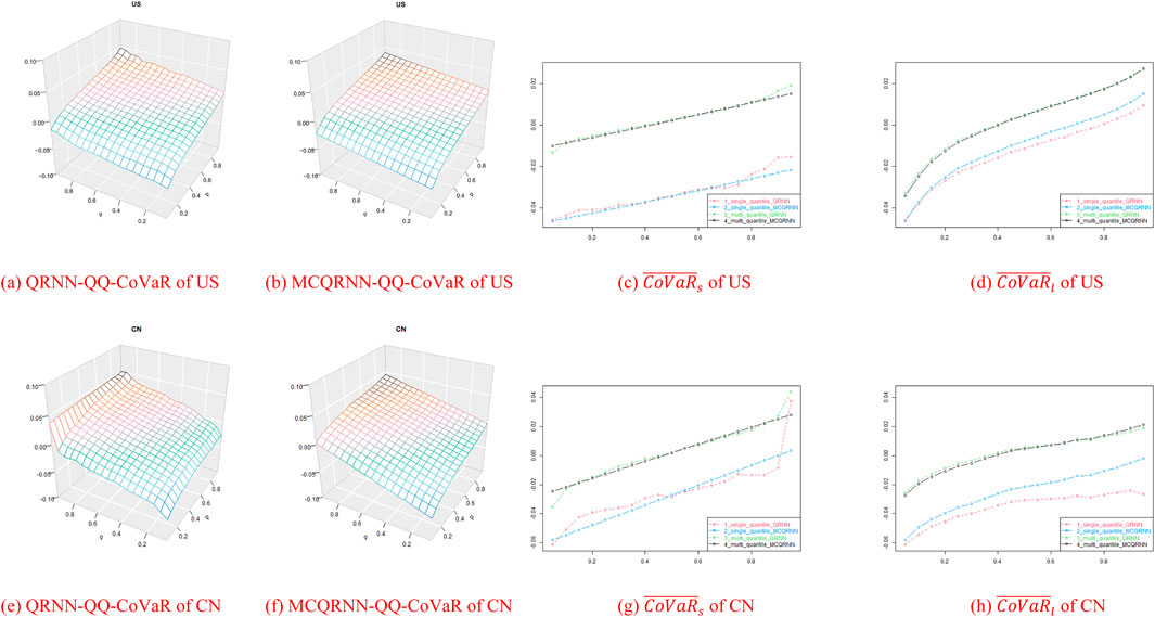
Figure 5. QQ-CoVaR surface and partial CoVaR curve of China and the United States. (A) QRNN-QQ-CoVaR of US, (B) MCQRNN-QQ-CoVaR of US, (C) ${\overline{CoVaR}}_s$ of US, (D) ${\overline{CoVaR}}_l$ of US, (E) QRNN-QQ-CoVaR of CN, (F) MCQRNN-QQ-CoVaR of CN, (G) ${\overline{CoVaR}}_s$ of CN, and (H) ${\overline{CoVaR}}_l$ of CN.

By comparing the $QRNN-QQ-CoVaR$ surfaces in Figures 5A, B and $MCQRNN-QQ-CoVaR$ in Figures 5E, F, it is found that the surface calculated by $MCQRNN$ is smoother than that calculated by $QRNN$. That means less bias in $CoVaR$ calculations for an extreme quantile, such as $q=0.95,$ by $MCQRNN$. On the same axis scale, the surface of the United States is flatter, which means fewer sensitivities to the quantile of stand-alone risk.

The reasons for the differences between China and the United States are market structure, investor base, and risk distribution. The American market is the largest and most diversified in the world, with companies representing a wide array of industries and sectors. This diversification helps to mitigate stand-alone risks associated with individual companies, sectors, or events. Additionally, American institutional investors like mutual funds, pension funds, and hedge funds play a significant role. These institutions usually employ sophisticated risk management strategies, including diversification and hedging, which further diminish sensitivity to stand-alone risks. Furthermore, the US market offers a wide array of financial instruments, such as options, futures, and swaps, that allow for the hedging of specific risks. This availability of hedging tools enables market participants to isolate and manage stand-alone risks effectively. Because the $CoVaR$ estimated $QRNN$ is based on each quantile separately, there is a non-monotonic trend with the change of $q$ quantile in Figure 5E. In order to compare the differences between $QRNN$ and $MCQRNN$ in different conditions, we analyze the $CoVaR$ of single quantiles and multi-quantiles separately.

Considering that $CoVaR$ in this paper takes into account two quantiles, partial $CoVaR$ in two directions are shown in Figures 5C, D according to Equation 11. On the one hand, as shown in Figure 5C, the red line and the blue line respectively represent the $CoVaR$ calculated by $QRNN$ and $MCQRNN$, when the $p_l$ quantile is 0.01. Meanwhile, the green and gray line respectively represent the average level of $CoVaR$ calculated by $QRNN$ and $MCQRNN$ at each $p_l$ quantile. In extreme conditions, the blue line tends to be a straight line, while the red line fluctuates around it. The phenomenon of “quantile crossing” occurs when the $CoVaR$ of $q_s=0.45$ is higher than that of $q_s=0.5$, which indicates that $MCQRNN$ is more robust than $QRNN$. The “quantile crossing” problem is weakened at the average level as shown in green line. On the other hand, as shown in Figure 5D, four lines respectively represent partial $CoVaR$ exposed to the entire risk, which states nonlinear characteristics. The results of $MCQRNN$ and $QRNN$ are similar at the average level, as shown by the green and gray lines in Figure 5. However, under extreme conditions, the red lines are always below the blue lines, and the phenomenon of quantile crossing still appears. Therefore, the improved $CoVaR$ calculated by $MCQRNN$ is more robust when considering multiple and two-sided quantiles to avoid the “quantile crossing” problem.

3.3 Analysis of composite risk spillovers

3.3.1 Network analysis of composite risk spillovers

According to Equation 8, after the estimation of $CoVaR$, the composite risk spillover can be obtained as the adjacency matrix ${\left[{\overline{\delta }}^{ji}\right]}_{N\times N}$ shown in Figure 6 and the network graph shown in Figure 7. In order to draw the risk spillover network maps across $N$ markets, the adjacency matrix ${\left[{\overline{\delta }}^{ji}\right]}_{N\times N}$ can be obtained by the average level of sample period ${\left[{\overline{\delta }}^{ji}\right]}_{N\times N}$. A weighted directed network can be plotted on the basis of this adjacency matrix.

Figure 6

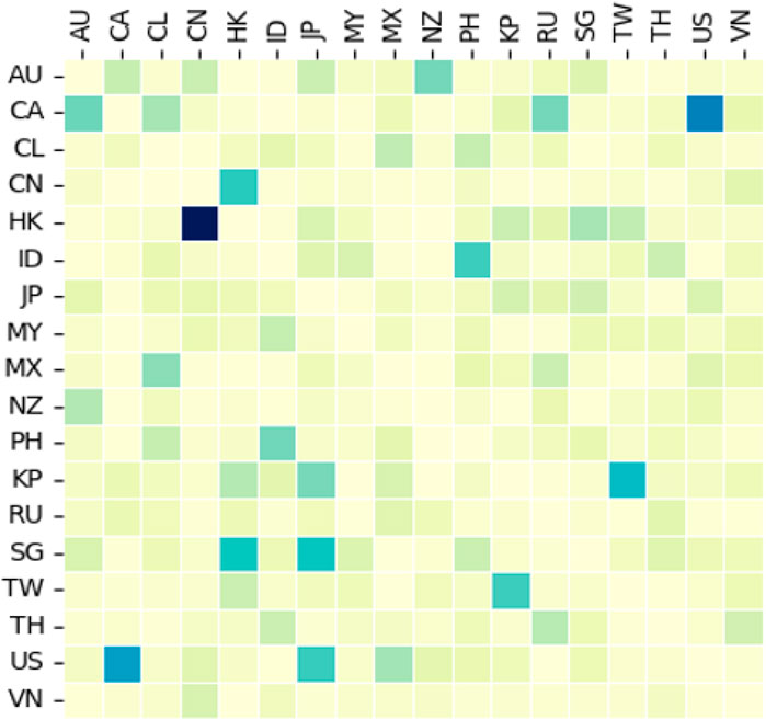
Figure 6. Heatmap of composite risk spillover in the overall period.

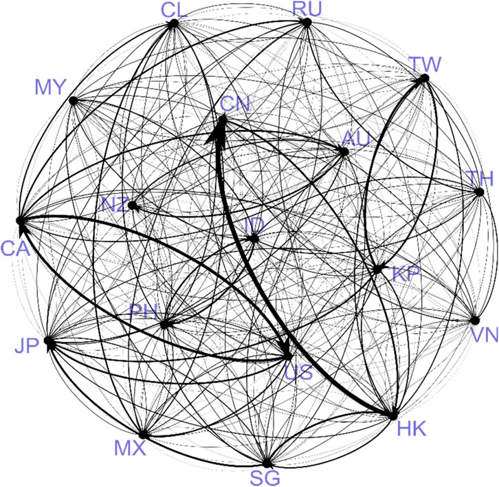
Figure 7

Figure 7. ${\overline{\delta }}^{ji}$ of composite risk spillover in the overall period.

As shown in Figure 6, each cell of the matrix represents a risk spillover correlation between the two markets. Where the color is darker, the level of risk spillover represented by the cell is higher. The cells with relatively dark colors in the graph are, respectively, the risk spillovers of HK →CN, CA →US, and US →CA. The mutual risk spillover between the United States and Canada can be explained by their geographical location, economic connections, and political policies. Canada is adjacent to the United States, and the two countries have a very close political relationship and an active trade association. Similar to the US and CA, the geographical location and economic connections between CN and HK are quite tight. However, the risk spillover level of HK →CN is the highest, while that of CN →HK is much lower. It is obvious that the high level of risk spillover effect from Hong Kong to the mainland China is due to the economic linkage between the two countries and the effect of Shanghai-Hong Kong Stock Connect program. In contrast, the economic policy of the Chinese system is different from that of western systems. The financial institutions in mainland China are not aggressive in investing. Moreover, the trade from mainland China to Hong Kong concentrates on domestic goods, which are at low prices. Those goods are why the risk spillover from CN to HK is relatively low. Therefore, the Hong Kong stock market is more mature and less susceptible to shocks.

In the following, we present a two-way weighted network to analyze systemic risks with a clearer visual structure. First, the adjacency matrix needs to be read via the NetworkX package in Python. Figure 7 shows a network map using the mean value of the samples. The arrow indicates the direction of the risk spillover. Both the size of the arrow and the width of the line segment indicate the intensity of risk spillover. Note that the width of the line segment states the level of the spillover of the larger one in the two-way relationship, in which the thinner one is covered. Therefore, the level of the risk spillover can only be judged based on the arrows in the comparison of two-way relationships. As can be seen, the most prominent line segment in this map is from HK to CN because of the Shanghai-Hong Kong Stock Connect and Shenzhen-Hong Kong Stock Connect programs. The level of risk spillover between the United States and Canada is also high, but the two-way relationship is symmetrical with almost equal size arrows. Similar two-way relationships also exist between TW and KP, JP and KP, ID and PH, and AU and CA. Such two-way relationships can be explained by the frequent trade interactions. It implies that stock markets are not only barometers of the economy but also effective reflections of the economic trades and global value chains through risk spillovers among financial markets.

Figure 8 is a frequency histogram of the risk spillover relationships. Four colors represent four algorithms adopted in calculating the risk spillover. The intensity of risk spillovers can be seen to exhibit a right-skewed spike with a thick tail. This indicates that while most risk spillovers are at low levels, the risk in extreme conditions is substantially outside the average range. In addition, the distribution of the red line is relatively flat, which means the risk spillover may be overestimated by $QRNN$ at a single quantile. The results of the remaining three algorithms are similar, though the peak of the green line is slightly skewed to the right.

Figure 8

Figure 8. Distribution of ${\overline{\delta }}^{ji}$ of composite risk spillover in the overall period.

3.3.2 Comparison of composite risk spillover calculated by QRNN and MCQRNN

A 3D-mesh surface is also employed to illustrate the one-way spillover from Hong Kong to mainland China, which is the most significant correlation in the Asia–Pacific region. As can be seen from the result from $QRNN$ Figure 9A, the ${\overline{d}}_{ls}^{ji}$ from Hong Kong to the mainland is fluctuating and outstanding at the extreme quantile $q_s=0.95$. However, as shown in Figure 9B, $MCQRNN$ can show relatively gentle overflow changes, especially showing no mutation characteristics at the extreme level. Similar to the algorithm comparison diagram of $CoVaR$ in Figure 5, it can be seen from Figure 9C that spillover levels represented by the blue and gray lines are more stable than those of the red and green lines. Meanwhile, the extreme situation of $q_s=0.95$ does not appear. This suggests that the estimators at the extreme quantile may be very sensitive to outliers under the partial differential spillover method. In contrast, $MCQRNN$ can both make the estimation results of $CoVaR$ more robust and obtain a more accurate assessment of the overflow level. In addition, from Figures 9C, D, the partial spillover increases with the decline of quantile $q_s$ and $p_l$; that is, during the challenging period, the risk spillover from Hong Kong to Chinese mainland is higher.

Figure 9

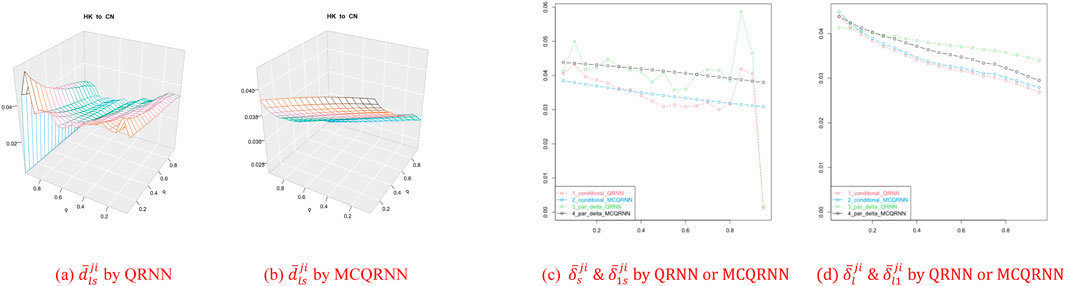
Figure 9. Risk spillover from HK to CN and partial indicators. (A) ${\overline{d}}_{ls}^{ji}$ by QRNN, (B) ${\overline{d}}_{ls}^{ji}$ by MCQRNN, (C) ${\overline{\delta }}_s^{ji}$ & ${\overline{\delta }}_{1s}^{ji}$ by QRNN or MCQRNN, and (D) ${\overline{\delta }}_l^{ji}$ & ${\overline{\delta }}_{l1}^{ji}$ by QRNN or MCQRNN.

3.3.3 Trend of total composite overflow indicator

To compare the overflow dynamic throughout the sample period, the time series diagram is drawn in Figure 10. Four lines in various colors represent the overall overflow levels of the two algorithms at the extreme level or the average level, based on the computational method of ${\mathrm{\Pi }}_t$ in Section 2.4.

Figure 10

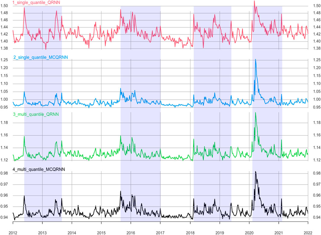
Figure 10. Total composite overflow indicator of the Asia–Pacific stock markets.

Compared with the composite overflow indicators calculated by the multi-quantile algorithm (in green and gray), the peak of overflow levels in the extreme condition represented by the red and blue lines are relatively higher because the peaks of overflow levels at the multi-quantile are flattened by averaging. Moreover, although spillover instability under extreme quantile conditions is reduced, the fluctuations of overflow calculated by the $MCQRNN$ method reveal more significance during periods of higher systemic risk. In other words, $MCQRNN$ also presents more robust and significant results even when calculating overflow under extreme conditions. The most prominent period was during the COVID-19 pandemic, which showed a higher level of spillover than other periods. Under the influence of this extreme event, the global real economy has stagnated, and production has been interrupted, leading to investor panic and insufficient investment confidence. Therefore, risk accumulates, and global asset prices fall. In contrast, the peak value calculated by $QRNN$ at a single quantile in this period is not different from that in other periods. Therefore, the single-quantile $QRNN$ method is worse than others.

Although the fluctuations of each line are different, there are four significant periods with high overall composite overflow levels. The first period is from May 2012 to September 2013, which corresponds to the EU debt crisis and the US stock market crash. The second period is in the second half of 2015 before the Chinese stock market crash occurred. The third period begins in 2018, which corresponds to the Sino-American trade war. The last fluctuant period is from March 2020 to February 2021, which is caused by the outbreak of COVID-19.

3.4 Comparison of systemic risk models

In this part, we analyze the average overflow of each market to the systemic ${\overline{\mathrm{\Phi }}}^j$, and their suffering ${\overline{\mathrm{\Gamma }}}^i$, relying on the methodology in⁸ Section 2.4.

The suffering indicators ${\overline{\mathrm{\Gamma }}}^i$ and the overflow indicators ${\overline{\mathrm{\Phi }}}^j$, which are respectively calculated by single-$QRNN$, multi-$QRNN$, single-$MCQRNN$, and multi-$MCQRNN$, are drawn as bar charts in Figure 11. As the legend shows, the suffering indicators ${\overline{\mathrm{\Gamma }}}^i$ are in light color and on the left side of each market, while the overflow indicators ${\overline{\mathrm{\Phi }}}^j$ are darker and on the right side. In addition, the $CoVaR$ calculated by $QRNN$ and $MCQRNN$ are illustrated as light and dark orange in the secondary axis. It is obvious that the light red bars stand out, indicating that China suffers the highest risk overflow when the ${\overline{\mathrm{\Gamma }}}^i$ calculated by $QRNN$ at a single quantile. However, when the algorithm is substituted by $MCQRNN$ with multiple quantiles, China is no longer the highest suffering market. In addition, the $CoVaR$ obtained by $QRNN$ and $MCQRNN$ are relatively close, and the $CoVaR$ of each market states no significant correlation with both ${\overline{\mathrm{\Phi }}}^j$ and ${\overline{\mathrm{\Gamma }}}^i$ indicators.

Figure 11

Figure 11. Composite systemic risk of each market.

Although Figure 11 shows differences in index calculations under the four algorithms, the comprehensive index is smaller than that calculated by a single sub-site. Whether under single or multi-component sites, the exponents obtained by the $MCQRNN$ algorithm are all smaller than those obtained by the $QRNN$ algorithm. In order to investigate whether the results of algorithms affect the ranking of systemic risk in each market, we also list the top ten markets of systemic risk index under various algorithms. As shown in Table 4, markets with higher risk overflow ${\overline{\mathrm{\Phi }}}^j$ are HK, CA, US, and SG. This result is consistent with the global financial markets’ practical experiences. In contrast, JP, CN, HK, and PH suffer more systemic risk because of the higher ${\overline{\mathrm{\Gamma }}}^i$. On the one hand, this may be related to the fact that these countries are more dependent on trade exports and have poor economic resilience, resulting in suffering more risk overflow. On the other hand, higher ${\overline{\mathrm{\Gamma }}}^i$ may also indicate that investors in these stock markets react strongly to the shocks. Compared with $MCQRNN$, the ${\overline{\mathrm{\Gamma }}}^i$ of China is driven higher than it calculated by $QRNN$, which means that the $MCQRNN$ method weakens the impact of the extreme condition.

Table 4

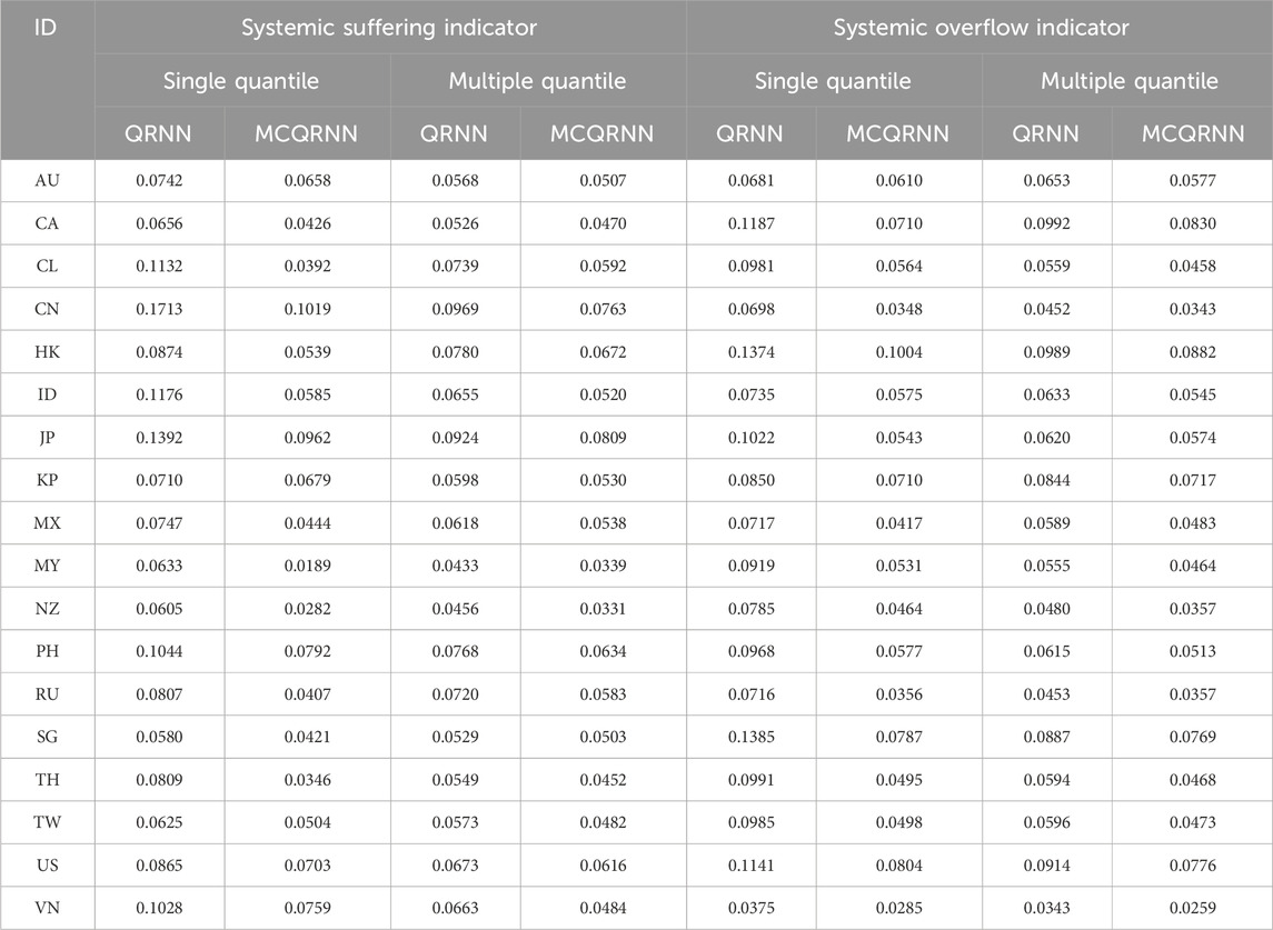
Table 4. Composite systemic risk indicators of each market.

4 Discussion and conclusion

To improve the traditional paradigm of risk spillovers among financial markets, this paper has calculated a multi-quantile $CoVaR$ based on $MCQRNN$. This study broadens the perspective of risk spillover research to financial market indexes and takes into account both the analysis of tail risk spillovers and risk spillovers under normality. The following conclusions were drawn based on empirical analyses of the Asia–Pacific region:

First, by visualizing the partial $CoVaR$, the “quantile crossing” problem is found on the estimation of $CoVaR$ but can be relieved by $MCQRNN$. This issue can be described as “a worse condition may cause less risk loss.” It is not only a logical problem but also reveals that $CoVaR$ may be sensitive to quantile selection. Fortunately, this problem rarely occurs on ${CoVaR}_l$ at the quantile of exposure risk state and can be relieved by substituting $MCQRNN$ for $QRNN$. On the other hand, through the estimation of partial ${CoVaR}_l$ at the other side quantile, the non-linear characteristic of each market is visualized. Different from the $CoVaR$ at the stand-alone risk state, the value at risk declines rapidly when exposed risk rises to an extreme state. This concludes that the non-linear algorithm is suitable for estimating $CoVaR$ precisely without over-fitting.

Second, the overestimation of spillover may occur when calculated by $QRNN$ at a single quantile, compared with $MCQRNN-QQ$ or at multiple quantiles. Based on the comparison of two 3D-mesh surfaces and the line charts of partial $\delta$ of four algorithms, the over-fitting in extreme conditions may contribute to the overestimation of composite spillover. The estimation of $QRNN$ at a single quantile shows less robustness than other three algorithms in the trend chart of total composite overflow.

Third, the stock market in mainland China is highly exposed to the risk spillovers from the Hong Kong stock market. In addition to the short geographical distance between them, another reason for this relatively asymmetric risk spillover may be that investors in mainland China are more concerned about the opposite, but investors in Hong Kong are more independent and have more complete information. In addition, the mutual spillovers between the United States and Canada are also significant, which may be due to the special geographic relationship between the United States and Canada as well as tight trade cooperation and economic dependency between two markets. Cross-market comparisons show that the model supports the traditional view that Hong Kong, Canada, United States, and Singapore are more important markets in the Asia–Pacific region. In contrast, the Chinese mainland and Japanese markets received the most spillovers during the sample period.

This paper studies the systemic risk and risk spillover under multiple quantiles, providing a reference for stock investment and risk regulation in the Asia–Pacific market. This method can not only be applied to the study of inter-institutional risk spillover but can also be helpful in capturing the nonlinear characteristics of individuals’ systemic risk. However, this paper still has some shortcomings. Limited by the time and space complexity of the algorithms, it is impossible to use the rolling window to estimate and calculate the daily samples. Therefore, the out-of-sample prediction effect of the model cannot be investigated. Further study is needed to improve the efficiency of the model and expand the sample.

Data availability statement

The original contributions presented in the study are included in the article/Supplementary Material; further inquiries can be directed to the corresponding author.

Author contributions

CR: conceptualization, investigation, methodology, software, supervision, writing–original draft, and writing–review and editing. ZZ: conceptualization, formal analysis, investigation, resources, and writing–original draft. DZ: formal analysis, investigation, resources, and writing–original draft.

Funding

The author(s) declare that financial support was received for the research, authorship, and/or publication of this article. This research is funded by the National Nature Science Foundation of China (NSFC), grant number 72173018; the Humanity and Social Science Research Project of Anhui Educational Committee, grant number 2024AH052470; and the High-level Talent Research Initiation Project at Anhui Business College, grant number 2024KYQD05.

Conflict of interest

The authors declare that the research was conducted in the absence of any commercial or financial relationships that could be construed as a potential conflict of interest.

Publisher’s note

All claims expressed in this article are solely those of the authors and do not necessarily represent those of their affiliated organizations, or those of the publisher, the editors, and the reviewers. Any product that may be evaluated in this article, or claim that may be made by its manufacturer, is not guaranteed or endorsed by the publisher.

Supplementary material

The Supplementary Material for this article can be found online at: https://www.frontiersin.org/articles/10.3389/fphy.2024.1484589/full#supplementary-material

Footnotes

¹“Higher risk but less loss” means the greater the risk, the smaller the loss because of the quantile crossing.

²${\mathrm{q}}_{\mathrm{s}}$ is the stand-alone level; $-\mathrm{i}$ of ${\mathrm{R}}_{\mathrm{t}}^{-\mathrm{i}}$ is a vector.

³${\mathrm{p}}_{\mathrm{l}}$ represents the conditional exposed risk.

⁴$-\mathit{i}$ in $\mathit{C}\mathit{A}\mathit{V}\mathit{i}\mathit{a}{\mathit{R}}_{\mathit{l},\mathit{t}}^{-\mathit{i}}$ is a vector, which is the same as ${\mathit{R}}_{\mathit{t}}^{-\mathit{i}}$ in Equation 2.

⁵MQ-CAViaR charts for other stock markets are shown in Supplementary Appendix Figure SA1.

⁶Supplementary Appendix Figure SA2 presents the QRNN-QQ-CoVaR 3D-surface plots for other market indexes.

⁷Supplementary Appendix Figure SA3 represents the stand-alone $\text{CoVaR}$ plots for other market indexes. Supplementary Appendix Figure SA4 represents the exposed partial $\text{CoVaR}$ plots for other market indexes.

⁸In Section 3.4, we calculate the average values for ${\mathit{\Gamma }}_{\mathit{t}}^{\mathit{i}}$ and ${\mathit{\Phi }}_{\mathit{t}}^{\mathit{j}}$, respectively. The equations are ${\overline{\mathit{\Gamma }}}^{\mathit{i}}=\frac{1}{\mathit{T}}{\displaystyle \sum _{\mathit{t}=1}^{\mathit{T}}}{\mathit{\Gamma }}_{\mathit{t}}^{\mathit{i}}$ and ${\overline{\mathit{\Phi }}}^{\mathit{j}}=\frac{1}{\mathit{T}}{\displaystyle \sum _{\mathit{t}=1}^{\mathit{T}}}{\mathit{\Phi }}_{\mathit{t}}^{\mathit{j}}$.

References

1. Allen F, Carletti E. What is systemic risk? J Money, Credit Banking (2013) 45:121–7. doi:10.1111/jmcb.12038

CrossRef Full Text | Google Scholar

2. Allen F, Gale D. Financial contagion. J Polit Economy (2000) 108:1–33. doi:10.1086/262109

CrossRef Full Text | Google Scholar

3. Acemoglu D, Carvalho VM, Ozdaglar A, Tahbaz-Salehi A. The network origins of aggregate fluctuations. Econometrica (2012) 80:1977–2016. doi:10.3982/ECTA9623

CrossRef Full Text | Google Scholar

4. Acemoglu D, Ozdaglar A, Tahbaz-Salehi A. Systemic risk and stability in financial networks. Am Econ Rev (2015) 105:564–608. doi:10.1257/aer.20130456

PubMed Abstract | CrossRef Full Text | Google Scholar

5. Elliott M, Golub B, Jackson MO. Financial networks and contagion. Am Econ Rev (2014) 104:3115–53. doi:10.1257/aer.104.10.3115

CrossRef Full Text | Google Scholar

6. Greenwood R, Landier A, Thesmar D. Vulnerable banks. J Financial Econ (2015) 115:471–85. doi:10.1016/j.jfineco.2014.11.006

CrossRef Full Text | Google Scholar

7. Engle R. Dynamic conditional correlation: a simple class of multivariate generalized autoregressive conditional heteroskedasticity models. J Business and Econ Stat (2002) 20:339–50. doi:10.1198/073500102288618487

CrossRef Full Text | Google Scholar

8. Rodriguez JC. Measuring financial contagion: a Copula approach. J Empirical Finance (2007) 14:401–23. doi:10.1016/j.jempfin.2006.07.002

CrossRef Full Text | Google Scholar

9. Billio M, Getmansky M, Andrew WL, Pelizzon L. Econometric measures of connectedness and systemic risk in the finance and insurance sectors. J Financial Econ (2012) 104:535–59. doi:10.1016/j.jfineco.2011.12.010

CrossRef Full Text | Google Scholar

10. Diebold FX, Yilmaz K. On the network topology of variance decompositions: measuring the connectedness of financial firms. J Econom (2014) 182:119–34. doi:10.1016/j.jeconom.2014.04.012

CrossRef Full Text | Google Scholar

11. Baruník J, Křehlík T. Measuring the frequency dynamics of financial connectedness and systemic risk. J Financial Econom (2018) 16:271–96. doi:10.1093/jjfinec/nby001

CrossRef Full Text | Google Scholar

12. Adrian T, Brunnermeier MK. CoVaR. Am Econ Rev (2016) 106:1705–41. doi:10.1257/aer.20120555

CrossRef Full Text | Google Scholar

13. Hautsch N, Schaumburg J, Schienle M. Financial network systemic risk contributions. Rev Finance (2015) 19:685–738. doi:10.1093/rof/rfu010

CrossRef Full Text | Google Scholar

14. Fan Y, Härdle WK, Wang W, Zhu L. Single-index-based CoVaR with very high-dimensional covariates. J Business and Econ Stat (2018) 36:212–26. doi:10.1080/07350015.2016.1180990 (Accessed July 17, 2024).

CrossRef Full Text | Google Scholar

15. Härdle WK, Wang W, Yu L. TENET: tail-Event driven NETwork risk. J Econom (2016) 192:499–513. doi:10.1016/j.jeconom.2016.02.013

CrossRef Full Text | Google Scholar

16. Keilbar G, Wang W. Modelling systemic risk using neural network quantile regression. Empir Econ (2022) 62:93–118. doi:10.1007/s00181-021-02035-1

CrossRef Full Text | Google Scholar

17. Naeem MA, Karim S, Tiwari AK. Quantifying systemic risk in US industries using neural network quantile regression. Res Int Business Finance (2022) 61:101648. doi:10.1016/j.ribaf.2022.101648

CrossRef Full Text | Google Scholar

18. Anwer Z, Khan A, Naeem MA, Tiwari AK. Modelling systemic risk of energy and non-energy commodity markets during the COVID-19 pandemic. Ann Oper Res (2022) 1–35. doi:10.1007/s10479-022-04879-x

CrossRef Full Text | Google Scholar

19. Xiao C, Xu X, Lei Y, Zhang K, Liu S, Zhou F. Counterfactual graph learning for anomaly detection on attributed networks. IEEE Trans Knowledge Data Eng (2023) 35:10540–53. doi:10.1109/TKDE.2023.3250523

CrossRef Full Text | Google Scholar

20. Li H-J, Feng Y, Xia C, Cao J. Overlapping graph clustering in attributed networks via generalized cluster potential game. ACM Trans Knowl Discov Data (2023) 18(27):1–26. doi:10.1145/3597436

CrossRef Full Text | Google Scholar

21. Bekiros S, Shahzad SJH, Arreola-Hernandez J, Ur Rehman M. Directional predictability and time-varying spillovers between stock markets and economic cycles. Econ Model (2018) 69:301–12. doi:10.1016/j.econmod.2017.10.003

CrossRef Full Text | Google Scholar

22. Dong Z, Li Y, Zhuang X, Wang J. Impacts of COVID-19 on global stock sectors: evidence from time-varying connectedness and asymmetric nexus analysis. The North Am J Econ Finance (2022) 62:101753. doi:10.1016/j.najef.2022.101753

CrossRef Full Text | Google Scholar

23. Ren Y, Tan A, Zhu H, Zhao W. Does economic policy uncertainty drive nonlinear risk spillover in the commodity futures market? Int Rev Financial Anal (2022) 81:102084. doi:10.1016/j.irfa.2022.102084

CrossRef Full Text | Google Scholar

24. El Adlouni S, Baldé I. Bayesian non-crossing quantile regression for regularly varying distributions. J Stat Comput Simulation (2019) 89:884–98. doi:10.1080/00949655.2019.1573899

CrossRef Full Text | Google Scholar

25. Huang Y. Restoration of monotonicity respecting in dynamic regression. J Am Stat Assoc (2017) 112:613–22. doi:10.1080/01621459.2016.1149070

PubMed Abstract | CrossRef Full Text | Google Scholar

26. Allen F, Carletti E. What is systemic risk? J Money, Credit Banking (2013) 45:121–7. doi:10.1111/jmcb.12038

CrossRef Full Text | Google Scholar

27. Acharya V, Pedersen L, Philippon T, Richardson M. Measuring systemic risk. The Rev Financial Stud (2017) 30:2–47. doi:10.1093/rfs/hhw088

CrossRef Full Text | Google Scholar

28. Catania L, Luati A. Semiparametric modeling of multiple quantiles. J Econom (2023) 237:105365. doi:10.1016/j.jeconom.2022.11.002

CrossRef Full Text | Google Scholar

29. Li Y, Luo J, Jiang Y. Policy uncertainty spillovers and financial risk contagion in the Asia-Pacific network. Pacific-Basin Finance J (2021) 67:101554. doi:10.1016/j.pacfin.2021.101554

CrossRef Full Text | Google Scholar

30. Lee K-J, Lu S-L, Shih Y. Contagion effect of natural disaster and financial crisis events on international stock markets. J Risk Financial Management (2018) 11:16. doi:10.3390/jrfm11020016

CrossRef Full Text | Google Scholar

31. Pavlova I, de Boyrie ME. Carry trades and sovereign CDS spreads: evidence from asia-pacific markets. J Futures Markets (2015) 35:1067–87. doi:10.1002/fut.21694

CrossRef Full Text | Google Scholar

32. Koenker R, Bassett G. Regression quantiles. Econometrica (1978) 46:33–50. doi:10.2307/1913643

CrossRef Full Text | Google Scholar

33. Taylor JW. A quantile regression neural network approach to estimating the conditional density of multiperiod returns. J Forecast (2000) 19:299–311. doi:10.1002/1099-131X(200007)19:4<299::AID-FOR775>3.0.CO;2-V

CrossRef Full Text | Google Scholar

34. Cannon AJ. Non-crossing nonlinear regression quantiles by monotone composite quantile regression neural network, with application to rainfall extremes. Stoch Environ Res Risk Assess (2018) 32:3207–25. doi:10.1007/s00477-018-1573-6

CrossRef Full Text | Google Scholar

35. Chen X, Shen X. Sieve extremum estimates for weakly dependent data. Econometrica (1998) 66:289–314. doi:10.2307/2998559

CrossRef Full Text | Google Scholar

36. Chen X, White H. Improved rates and asymptotic normality for nonparametric neural network estimators. IEEE Trans Inf Theor (1999) 45:682–91. doi:10.1109/18.749011

CrossRef Full Text | Google Scholar

37. Huber PJ. Robust statistics. In: Robust statistics. John Wiley and Sons, Ltd (2024) 297–305. doi:10.1002/9780470434697.ch13

CrossRef Full Text | Google Scholar

38. Bishop CM. The multi-layer perceptron. In: CM Bishop, Editor. Neural networks for pattern recognition. Oxford University Press (2024) 0. doi:10.1093/oso/9780198538493.003.0004

CrossRef Full Text | Google Scholar

39. Cannon AJ. Quantile regression neural networks: implementation in R and application to precipitation downscaling. Comput and Geosciences (2011) 37:1277–84. doi:10.1016/j.cageo.2010.07.005

CrossRef Full Text | Google Scholar

40. Cannon AJ. Non-crossing nonlinear regression quantiles by monotone composite quantile regression neural network, with application to rainfall extremes. Stoch Environ Res Risk Assess (2018) 32:3207–25. doi:10.1007/s00477-018-1573-6

CrossRef Full Text | Google Scholar

41. Engle RF, Manganelli S. CAViaR: conditional autoregressive value at risk by regression quantiles. J Business and Econ Stat (2004) 22:367–81. doi:10.1198/073500104000000370

CrossRef Full Text | Google Scholar

42. Buczyński M, Chlebus M. Is CAViaR model really so good in Value at Risk forecasting? Evidence from evaluation of a quality of Value-at-Risk forecasts obtained based on the: GARCH(1,1), GARCH-t(1,1), GARCH-st(1,1), QML-GARCH(1,1), CAViaR and the historical simulation models depending on the stability of financial markets. Faculty of Economic Sciences, University of Warsaw (2017). Available from: https://econpapers.repec.org/paper/warwpaper/2017-29.htm (Accessed August 2, 2024).

Google Scholar

43. Mullen KM, Ardia D, Gil DL, Windover D, Cline J. DEoptim: an R package for global optimization by differential evolution. J Stat Softw (2011) 40:1–26. doi:10.18637/jss.v040.i06

CrossRef Full Text | Google Scholar

44. Härdle WK, Wang W, Yu L. TENET: tail-Event driven NETwork risk. J Econom (2016) 192:499–513. doi:10.1016/j.jeconom.2016.02.013

CrossRef Full Text | Google Scholar

45. Xu Q, Deng K, Jiang C, Sun F, Huang X. Composite quantile regression neural network with applications. Expert Syst Appl (2017) 76:129–39. doi:10.1016/j.eswa.2017.01.054

CrossRef Full Text | Google Scholar