Infrared and visible image fusion based on multi-scale transform and sparse low-rank representation

Infrared and visible image sensors are wildly used and show strong complementary properties, the fusion of infrared and visible images can adapt to a wider range of applications. In order to improve the fusion of infrared and visible images, a novel and effective fusion method is proposed based on multi-scale transform and sparse low-rank representation in this paper. Visible and infrared images are first decomposed to obtain their low-pass and high-pass bands by Laplacian pyramid (LP). Second, low-pass bands are represented with some sparse and low-rank coefficients. In order to improve the computational efficiency and learn a universal dictionary, low-pass bands are separated into several image patches using a sliding window prior to sparse and low rank representation. The low-pass and high-pass bands are then fused by particular fusion rules. The max-absolute rule is used to fuse the high-pass bands, and max-L1 norm rule is utilized to fuse the low-pass bands. Finally, an inverse LP is performed to acquire the fused image. We conduct experiments on three datasets and use 13 metrics to thoroughly and impartially validate our method. The results demonstrate that the proposed fusion framework can effectively preserve the characteristics of source images, and exhibits superior stability across various image pairs and metrics.

1 Introduction

Due to the use of new application scenarios and the increasing demand for image sensors in fields such as transportation, security, and military, single image sensors are becoming less effective. Because source images from multiple sensors contain more detailed information and can meet more complex requirements, it is more effective to collect information about a particular situation using various image sensors. Infrared and visible image sensors are wildly used and show strong complementary properties. Visible image sensors have high spatial resolution, rich details, and contrast between light and dark, but they are susceptible to adverse environments like low lighting and fog. Infrared image sensors are less affected by environments but have low resolution and poor texture. Therefore, the combination of infrared and visible sensors can adapt to a wider range of applications.

Visible and infrared image fusion has attracted considerable attention. So far, fusion methods can be divided into conventional methods and deep learning-based methods on whether deep learning is utilized [1]. Conventional methods include spatial domain-based methods and transform domain-based methods. Spatial domain-based methods fuse images directly on pixels or image patches/blocks. However, these methods are susceptible to noise and it is easy to introduce artifacts. Zhang [2] proposed an effective infrared and visual image fusion algorithm through infrared feature extraction and visual information preservation, while Xiao [3] presented a spatial domain-based image fusion method based on fourth order partial differential equations and principal component analysis, Ma [4] proposed a novel fusion algorithm based on gradient transfer and total variation minimization; the gradient calculation is related to a specific matric. Transform domain-based methods firstly transform source images into another domain, and then fusion rules are used to fuse the source images. After the fusion is completed, the fused results are transformed back to image form. Many good results have been achieved with the transform domain-based method. Li [5] proposed a latent low-rank representation image fusion method that received very good results although it is time-intensive. Bavirisetti [6] achieved image fusion based on saliency detection and two scale image decomposition; they also studied anisotropic diffusion and Karhunen - Loeve transform for image fusion [7]. Kumar [8] used a cross-bilateral filter to extract the image details and achieved image fusion based on weighted average. Zhou [9] and Li [10] both studied the guided filter to achieve image fusion. Bavirisetti [11] used multi-scale image decomposition, structure transferring property, visual saliency detection, and weight map construction to fuse images. Naidu [12] studied multi-resolution singular value decomposition to fuse images. Qi [13] proposed a saliency-based decomposition strategy for infrared and visible image fusion. Considering the advantages in image information capture, some researchers have studied many hybrid methods by combining domain transform and some emerging image information processing algorithms. Zhou [14] studied a hybrid image fusion method through a hybrid multi-scale decomposition with Gaussian and bilateral filters. Liu [15] studied the effectiveness of image fusion by combing different transform methods and sparse representation; the results demonstrated that the combination of multi-scale transform (MST) and sparse representation achieved better results. Ma [16] used a rolling guidance filter and Gaussian filter to decompose source images, and an improved visual saliency map was proposed to fuse images. In order to eliminate the modal differences between infrared and visible images, Chen [17] utilized feature-based decomposition and domain normalization to improve the image fusion quality. Li [18] used rolling guidance filtering and a gradient saliency map to address the issue of brightness and detail information loss in infrared and visible image fusion.

As artificial intelligence continues to develop quickly, many deep learning methods are being examined for their use in visible and infrared image fusion. Liu [19] used convolution neural networks and Gaussian pyramid decomposition to compute a wight map—the wight map was used to fuse the Laplacian pyramid decomposed source images. Li [20] used a deep learning network to extract multi-layer features of detailed parts of source images and fused images by l1-norm and weighted-average strategy. Li [21] also studied the performance of ResNet and zero-phase component analysis. Zhang [1] comprehensively reviewed the current deep learning-based image fusion algorithms and established a benchmark. He also compared learning methods and non-learning methods and concluded that the performances of deep learning-based image fusion algorithms do not show superiority over non-learning algorithms [22]. Wei [23] proposed an attention-based dual-branch feature decomposition fusion network.

As discussed above, sparse representation has achieved good results in visible and infrared image fusion. Recent studies demonstrate that combining sparse and low-rank constraints can enhance the information capture of images [24,25], because low-rank constraints can recover some structural information of source images. In this paper, we aim at establishing a new visible and infrared image fusion method using sparse and low-rank representation. Considering the good performance of Laplacian pyramid (LP), source images are firstly transformed into another domain to obtain their low-pass and high-pass bands. Secondly, low-pass bands are represented as some sparse and low-rank coefficients. Then, specific fusion rules are adopted to fuse the low-pass and high-pass bands. Finally, an inverse LP is conducted to obtain the fused image.

The contributions of this paper include 1) combining sparse constraint and low-rank constraint to establish a sparse low-rank representation model to improve the performance of extracting the complex structural features; 2) precisely designing a solution strategy for the sparse low-rank representation model, which is essential for image fusion with high qualities; and 3) establishing a new infrared and visible image fusion method based on Laplacian pyramid and sparse low-rank representation, the experimental results of which proved the advantages in fusion quality and improved runtime performance compared to methods with similar fusion quality.

The rest of this paper is organized as follows. Section 2 first presents the sparse low-rank representation model. Our fusion method is presented in Section 3. In Section 4, the experimental results are listed and analyzed. Section 5 summarizes the conclusions of this paper.

2 Sparse low-rank representation model

2.1 Basic theory of sparse representation

Given a signal vector V, sparse representation of V can be formulated as

$\underset{\mathit{a},\mathit{D}}{\min }{‖\mathit{a}‖}_{0}subjectto{‖\mathbf{V}-\mathit{D}\mathit{a}‖}_2\le \epsilon ,(1)$

where a is the sparse coefficient of source image V, D is an unknown dictionary matrix to be learnt, ${‖·‖}_0$ and ${‖·‖}_2$ are L0 norm and L2 norm correspondingly, and $\epsilon >0$ is the error tolerance and is related to noise. The dictionary D can be efficiently solved by K-SVD, any source images can be sparsely represented with D.

As the L0 norm is nonconvex and Equation 1 is a NP-hard problem, some research proved that the results of L1 norm are equal with L0 norm if the sparsity of optimized a is near its true value [26]. Hence, the L1 norm is used rather than the L0 norm to establish the spare representation model in this paper.

2.2 Sparse low-rank representation

In actual practice, the noise item $\epsilon$ in Equation 1 is hard to know in advance, so we change Equation 1 with L1 norm as the following form:

$\underset{\mathit{a}}{\min }{‖\mathit{a}‖}_1+\lambda {‖\mathit{E}‖}_{2,1}subjectto\mathbf{V}=\mathbf{D}\mathit{a}+\mathit{E},(2)$

where E is the noise item and is expected to be kept as small as possible, λ is a trade-off parameter, and ${‖·‖}_{2,1}$ is L21 norm and measures the level of noise. Some research has shown that low-rank constraints can further capture the complex structural information [27]. If the rank is not too large, the rank can be measured with nuclear norm [28]. We aim to combine sparse and low-rank constraints to enhance the performance of infrared and visible image fusion, so Equation 2 is changed as

$\underset{\mathit{a}}{\min }{‖\mathit{a}‖}_1+\alpha {‖\mathit{a}‖}_{*}+\lambda {‖\mathit{E}‖}_{2,1}subjectto\mathbf{V}=\mathbf{D}\mathit{a}+\mathit{E},(3)$

where ${‖·‖}_{*}$ is the nuclear norm and measures the rank of a matrix and α is the balance parameter. The problem of Equation 3 is an optimization problem with constraint; we introduce the alternating direction method of multipliers (ADMM) [29] to solve Equation 3. We first introduce two auxiliary variables, ${\mathit{a}}_1,{\mathit{a}}_2$, and Equation 3 can be converted into

$\underset{\mathit{a}}{\min }{‖{\mathit{a}}_1‖}_1+\alpha {‖{\mathit{a}}_2‖}_{*}+\lambda {‖\mathit{E}‖}_{2,1}subjectto\mathbf{V}=\mathbf{D}\mathit{a}+\mathit{E},\mathit{a}={\mathit{a}}_1,\mathit{a}={\mathit{a}}_2.(4)$

Optimization of Equation 4 is equal to minimize the following augmented Lagrange multiplier (ALM) function L

$\begin{array}{l}\mathrm{L}={‖{\mathit{a}}_1‖}_1+\alpha {‖{\mathit{a}}_2‖}_{*}+\lambda {‖\mathit{E}‖}_{2,1}\\ +〈{\mathit{Y}}_1,\mathbf{V}-\mathbf{D}\mathit{a}-\mathit{E}〉+〈{\mathit{Y}}_2,\mathit{a}-{\mathit{a}}_1〉+〈{\mathit{Y}}_3,\mathit{a}-{\mathit{a}}_2〉\\ +\frac{\mu }{2}\left({‖\mathbf{V}-\mathbf{D}\mathit{a}-\mathit{E}‖}_F^2+{‖\mathit{a}-{\mathit{a}}_1‖}_F^2+{‖\mathit{a}-{\mathit{a}}_2‖}_F^2\right),\end{array}(5)$

where μ represents positive penalty parameters,Y₁, Y₂, and Y₃ are Lagrange multipliers, and ${‖·‖}_F$ denotes the Frobenius norm. There are four variables $\mathit{a},{\mathit{a}}_1,{\mathit{a}}_2,\mathit{E}$, and three Lagrange multipliers Y₁, Y₂, and Y₃ in Equation 5. ADMM iteratively optimizes each variable while the others are fixed. Equation 5 is divided into five subproblems to separately optimize each variable.

(I) Update a:

$\mathit{a}=\arg \underset{\mathit{a}}{\min }{‖\mathbf{V}-\mathbf{D}\mathit{a}-\mathit{E}+\frac{{\mathit{Y}}_1}{\mu }‖}_F^2+{‖\mathit{a}-{\mathit{a}}_1+\frac{{\mathit{Y}}_2}{\mu }‖}_F^2+{‖\mathit{a}-{\mathit{a}}_2+\frac{{\mathit{Y}}_3}{\mu }‖}_F^2.(6)$

Equation 6 is a convex optimization problem, and the solution can be calculated by taking the first partial derivatives to variable a and setting them to zero. Let ${\mathbf{G}}_1=\mathbf{V}-\mathit{E}+\frac{{\mathit{Y}}_1}{\mu },{\mathbf{G}}_2={\mathit{a}}_1-\frac{{\mathit{Y}}_2}{\mu },{\mathbf{G}}_3={\mathit{a}}_2-\frac{{\mathit{Y}}_3}{\mu }$, it is clear that the close form solution of Equation 6 is

$\mathit{a}={\left({\mathbf{D}}^{\mathrm{T}}\mathbf{D}+2\mathbf{I}\right)}^{-1}\left({\mathbf{D}}^{\mathrm{T}}{\mathbf{G}}_1+{\mathbf{G}}_2+{\mathbf{G}}_3\right).(7)$

(II) Update ${\mathit{a}}_1$:

${\mathit{a}}_1=\arg \underset{{\mathit{a}}_1}{\min }{‖{\mathit{a}}_1‖}_1+\frac{\mu }{2}{‖\mathit{a}-{\mathit{a}}_1+\frac{{\mathit{Y}}_2}{\mu }‖}_F^2.(8)$

The solution of ${\mathit{a}}_1$ can be efficiently calculated with a soft-shrinkage operator [30]. Let ${\mathit{G}}_4=\mathit{a}+\frac{{\mathit{Y}}_2}{\mu }$, the solution of Equation 8 can be obtained with the soft-shrinkage operator and has the following form:

${\mathit{a}}_1=sign\left({\mathit{G}}_{\mathit{4}}\right)\odot \max \left(\left|{\mathit{G}}_{\mathit{4}}\right|-\frac{1}{\mu },0\right),(9)$

where sign(·) is sign function and ⊙ is Hadamard product.

(III) Update ${\mathit{a}}_2$:

${\mathit{a}}_2=\arg \underset{{\mathit{a}}_2}{\min }\alpha {‖{\mathit{a}}_2‖}_{*}+\frac{\mu }{2}{‖\mathit{a}-{\mathit{a}}_2+\frac{{\mathit{Y}}_3}{\mu }‖}_F^2.(10)$

The problem in Equation 10 can be solved by the singular value thresholding scheme [31]. Let ${\mathit{G}}_5=\mathit{a}+\frac{{\mathit{Y}}_3}{\mu }$, the singular value decomposition of ${\mathit{G}}_5$ is ${\mathit{G}}_5={\mathit{U}\mathit{S}\mathit{V}}^{\mathrm{T}}$. Then, the solution of Equation 10 has the following form according to the singular value thresholding scheme:

${\mathit{a}}_2=\mathit{U}·sign\left(\mathit{S}\right)\odot \max \left(\left|\mathit{S}\right|-\frac{\alpha }{\mu },0\right)·{\mathit{V}}^{\mathrm{T}}.(11)$

(IV) Update E:

$\mathit{E}=\arg \underset{\mathit{E}}{\min }\lambda {‖\mathit{E}‖}_{2,1}+\frac{\mu }{2}{‖\mathbf{V}-\mathbf{D}\mathit{a}-\mathit{E}+\frac{{\mathit{Y}}_1}{\mu }‖}_F^2.(12)$

This sub-problem of Equation 12 can be efficiently solved by the half-quadratic optimization strategy [32]. Let ${\mathit{G}}_6=\mathbf{V}-\mathbf{D}\mathit{a}+\frac{{\mathit{Y}}_1}{\mu }$, this sub-problem of Equation 12 can be efficiently solved by the half-quadratic optimization strategy as

$\mathit{E}\left(:,\mathrm{i}\right)=\left\{\begin{array}{ll}\frac{{‖{\mathit{G}}_6\left(:,\mathrm{i}\right)‖}_2-\frac{\lambda }{\mu }}{{‖{\mathit{G}}_6\left(:,\mathrm{i}\right)‖}_2}{\mathit{G}}_6\left(:,\mathrm{i}\right),& {‖{\mathit{G}}_6\left(:,\mathrm{i}\right)‖}_2>\frac{\lambda }{\mu }\\ 0,& {‖{\mathit{G}}_6\left(:,\mathrm{i}\right)‖}_2\le \frac{\lambda }{\mu }\end{array}\right.,\mathrm{i}=1,...,\mathrm{k},(13)$

where $\mathit{E}\left(:,\mathrm{i}\right),{\mathit{G}}_6\left(:,\mathrm{i}\right)$ denote the i-th column of E and G₆.

(V) Update Lagrange multipliers Y₁, Y₂, and Y₃:

$\left\{\begin{array}{l}{\mathit{Y}}_1={\mathit{Y}}_1+\mu \left(\mathbf{V}-\mathbf{D}\mathit{a}-\mathit{E}\right)\\ {\mathit{Y}}_2={\mathit{Y}}_2+\mu \left(\mathit{a}-{\mathit{a}}_1\right)\\ {\mathit{Y}}_3={\mathit{Y}}_3+\mu \left(\mathit{a}-{\mathit{a}}_2\right)\end{array}\right.,(14)$

where μ increases dynamically from small values by μ = ρμ, and ρ is a positive value.

The sparse low-rank coefficient a in Equation 5 can be solved by iteratively calculating the above five subproblems and obtaining their solutions as shown in Equations 7, 9, 11, 13, 14.

3 Fusion method based on sparse low-rank representation

In this section, we introduce the proposed infrared and visible image fusion method in detail. The proposed method consists of two steps: image decomposition and feature fusion. LP is used to decompose images into low-pass and high-pass parts. Low-pass parts are a smooth version of source images; they are fused based on sparse low-rank representation. High-pass parts contain more details and the fusion is based on the max-absolute rule. The schematic diagram of the proposed fusion method is shown in Figure 1.

Figure 1

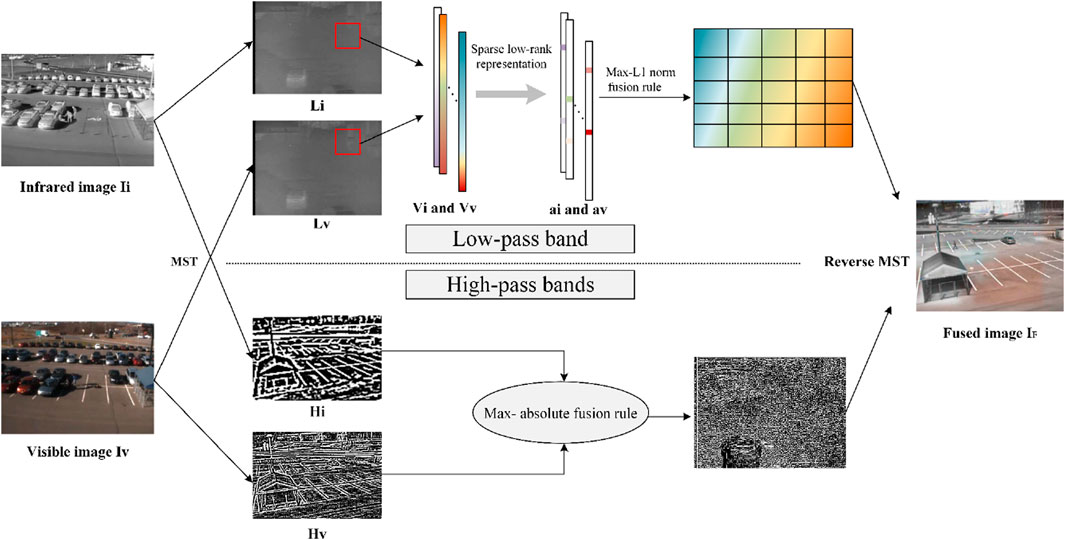
Figure 1. The schematic diagram of the proposed fusion method.

3.1 Image decomposition

MST is a popular transformation method and can transform the source images into a multi-scale domain. The source images are firstly transformed into a multi-scale domain by LP to obtain different information. Figure 2 shows the diagram of LP. In the first layer of decomposition, source image I is first convolved twice and down sampled once to obtain an interlayer result ${\mathbf{M}}_{\mathbf{d}}^{\mathbf{1}}$. The interlayer result ${\mathbf{M}}_{\mathbf{d}}^{\mathbf{1}}$ is used to compute the second interlayer result ${\mathbf{M}}_{\mathbf{d}}^2$ and the first high-pass band H₁. The second interlayer result ${\mathbf{M}}_{\mathbf{d}}^2$ for the next decomposition level is obtained by two convolutions and a down sampling. Meanwhile, after the interlayer result ${\mathbf{M}}_{\mathbf{d}}^{\mathbf{1}}$ goes through an up sampling and two convolutions, a high-pass interlayer result HP₁ is obtained. The first high-pass band H₁ can be calculated by subtracting the high-pass interlayer result HP₁ from source image I. In following i-th layer decomposition, similar conductions to those in the first layer are performed on the interlayer result ${\mathbf{M}}_{\mathbf{d}}^{\mathit{i}}\left(i=1,2,...,n\right)$ from the previous decomposition. The single difference is that, in the subtraction, the high-pass interlayer result HP_i is subtracted from the interlayer result ${\mathbf{M}}_{\mathbf{d}}^{\mathit{i}-\mathbf{1}}$ from the previous level subtracts to calculate the i-th high-pass band H_i. After n layers of decompositions, one low-pass band L and n high-pass bands H₁, H₂, … , H_n can be obtained; the number of high-pass bands is equal to the layers of decomposition.

Figure 2

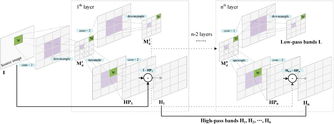
Figure 2. Diagram of image decomposition.

3.2 Fusion strategy

After the decomposition is completed and the low-pass bands and high-pass bands are obtained, the fusion step is conducted. Different fusion strategies are used to deal with low-pass bands and high-pass bands.

3.2.1 Fusion strategy of low-pass bands

The low-pass bands of infrared and visible image are represented by L_A and L_B; they are fused based on sparse low-rank representation. The sparse low-rank coefficients of L_A and L_B are firstly computed according to Equation 6. In order to improve the computing efficiency, the low-pass bands are divided into several image patches of size $\sqrt{n}\times \sqrt{n}$ by a sliding window. The sliding window slides from the top left to the bottom right and the step size of the sliding window is set as s pixels. In order to avoid block effect and keep enough overlap between different patches, the step size is less than the patch size. However, the step size cannot be too small or the overlapping region will be smoothed. Suppose there are k patches for L_A and L_B, each patch is represented as Pⁱ (i = 1, 2, … , k). In the following procedure, every patch is rearranged in column vector form, and the column vector of Pⁱ is marked as ${\mathbf{V}}^i\in {\mathbf{R}}^{n\times 1}$.

In order to further improve the computing efficiency, the column vector Vⁱ (i = 1, 2, … , k) is not directionally input into our sparse low-rank representation model. Firstly, the column vector Vⁱ is zero-averaged as follows

${\widehat{\mathbf{V}}}^i={\mathbf{V}}^i-{\overline{\mathrm{V}}}^i·\mathbf{1},(15)$

where ${\widehat{\mathbf{V}}}^i$ is zero-averaged patch, ${\overline{\mathrm{V}}}^i$ is the mean value of Vⁱ, and 1∈R^n×1 is an all-one vector. Then, ${\widehat{\mathbf{V}}}^i$ is used to solve the sparse low-rank coefficient. According to Equation 5, the optimization model can be expressed as

$\underset{\mathit{a}}{\min }{‖{\mathit{a}}_1^i‖}_1+\alpha {‖{\mathit{a}}_2^i‖}_{*}+\lambda {‖\mathit{E}‖}_{2,1}subjectto{\widehat{\mathbf{V}}}^i=\mathbf{D}{\mathit{a}}^i+\mathit{E},{\mathit{a}}^i={\mathit{a}}_1^i,\mathit{a}={\mathit{a}}_2^i,(16)$

It is worth noting that dictionary D is learnt based on ${\widehat{\mathbf{V}}}^i$, and ${\widehat{\mathbf{V}}}^i$ only contains the structural information. Therefore, the learnt D by Equation 1 is a universal dictionary and it can be used for any specific transform domain or parameter setting. Besides, because D is trained with the image patches ${\widehat{\mathbf{V}}}^i$ rather than whole images, D can keep a small size, which is important to deduce the requirements of computers and improve the solving efficiency.

Let ${\mathbf{V}}_A^i$ and ${\mathbf{V}}_B^i$ be the i-th patch of L_A and L_B in column vector form, the sparse low-rank coefficients ${\mathit{a}}_A^i,{\mathit{a}}_B^i$ of L_A and L_B can be obtained by Equations 15 and 16. Then the max-L1 norm rule is used to fuse ${\mathit{a}}_A^i$ and ${\mathit{a}}_B^i$, and the fused sparse low-rank coefficient ${\mathit{a}}_F^i$ can be obtained by

${\mathit{a}}_F^i=\left\{\begin{array}{cc}{\mathit{a}}_A^i,& {‖{\mathit{a}}_A^i‖}_1>{‖{\mathit{a}}_B^i‖}_1\\ {\mathit{a}}_B^i,& \text{else}\end{array}\right.,i=1,...,\mathrm{k},(17)$

and the fused patch ${\mathbf{V}}_F^i$ can be obtained by

${\mathbf{V}}_F^i=\mathbf{D}{\mathit{a}}_F^i+{\overline{\mathrm{V}}}_F^i·\mathbf{1},i=1,...,\mathrm{k},(18)$

where ${\overline{\mathrm{V}}}_F^i$ is an average. If ${‖{\mathit{a}}_A^i‖}_1>{‖{\mathit{a}}_B^i‖}_1$, ${\overline{\mathrm{V}}}_F^i$ takes as the average of ${\mathbf{V}}_A^i$, otherwise ${\overline{\mathrm{V}}}_F^i$ is the average of ${\mathbf{V}}_B^i$. After all k patches are fused with Equations 17, 18, each patch in the column vector form is converted to two-dimensional form. All the two-dimensional patches are spliced to obtain the fused low-pass bands L_F.

3.2.2 Fusion strategy of high-pass bands

The high-pass bands are directly fused based with the max-absolute rule. There are n high-pass bands and every high-pass band pair is fused separately. The absolute value of high-pass band H_i (i = 1, 2, … , n) is first computed. Then, the absolute value goes through 2-D order-statistic filtering. The filtering results of visible and infrared high-pass bands are compared directly. The bigger is reserved and the smaller is discarded. The fused high-pass band ${\mathbf{H}}_{\mathbf{F}}^{\mathit{i}}$ can be obtained by adding the comparation results. The detailed information can be seen in [33].

3.3 Reconstruction of fused image

After L_F and H_F are obtained, a reverse LP is conducted to reconstruct the fused image I_F. The diagram of reconstruction is shown in Figure 3. The reconstruction is the reverse operation of decomposition, there are also n layers of reconstruction. The low-pass band L_F firstly goes through an upsampling and two convolutions, and we can obtain an interlayer result ${\mathbf{M}}_{\mathbf{r}}^{\mathbf{1}}$. The interlayer result ${\mathbf{M}}_{\mathbf{r}}^{\mathbf{1}}$ is added to the n-th fused high-pass band ${\mathbf{H}}_{\mathbf{F}}^{\mathbf{n}}$, and the sum result is transferred into the second layer. In every following reconstruction layer, a similar operation is conducted. The only difference is that the high-pass band of each layer is used in the additional operation. In the n-th layer of reconstruction, the fused image I_F can be reconstructed by adding the interlayer result ${\mathbf{M}}_{\mathbf{r}}^{\mathbf{n}}$ and the first fused high-pass band ${\mathbf{H}}_{\mathbf{F}}^{\mathbf{1}}$.

Figure 3

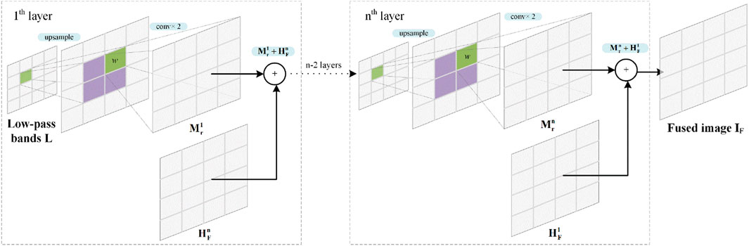
Figure 3. Diagram of fused image reconstruction.

4 Experiments and evaluation

In this section, we verify and analyze our method through extensive experiments. All the experiments were performed on a desktop with Windows 10 operating system, 11th Gen Intel(R) Core (TM) i7-11700F @ 2.50 GHz CPU, and 16 GB RAM. In our method, the level of decomposition is 4, both of a, and λ is 1e-5. It is noteworthy that the convolution kernel is the same across all the convolution layers, because the impact of convolution kernels is much weaker than the number of decomposition layers [15]. The convolution kernel in the following experiments is a Gauss filter [1 4 6 4 1]/16.

4.1 Experimental setups

4.1.1 Source images

In order to verify the effectiveness and analyze the characteristics of our method, three open access visible and infrared image datasets are adopted in the following experiments, namely, VIFB [22], TNO [34], LLVIP [35]. In VIFB, there are 21 pairs of visible and infrared images. In TNO, there are 37 image pairs; the resolution of images is 640 × 480. In LLVIP, there are 50 image pairs for validation and the images are mainly taken in dark environments.

4.1.2 Objective evaluation metrics

The metrics of image fusion can be divided into four types: information theory-based, image feature-based, image structural similarity-based, and human perception-based [22]. To evaluate and compare performance comprehensively and objectively, 13 evaluation metrics are used in the following experiments. The 13 metrics and their meaning are listed in Table 1. Considering that there are two source images and a single fused image, the 13 metrics can be categorized into three types based on their calculation methods: metrics independent of the source images, metrics computed separately on the fused and source images and then averaged, and metrics computed separately on the fused and source images and then summed. All the calculation methods are based on [15]. Metrics, including AG, EI, EN, SF, and SD, belong to the first category. The second type of metrics includes PSNR, Q^AB/F, Q^CB, Q^CV, and RMSE, and the rest of the metrics are categorized into the third type.

Table 1

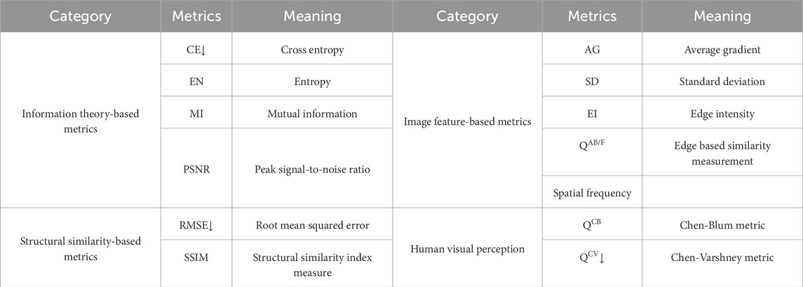
Table 1. The 13 metrics and their meaning in the following experiments. ‘‘↓’’ means that smaller value denotes better results.

4.2 Experiment results on VIFB dataset

The proposed method is first tested on the VIFB dataset and compared with 20 kinds of methods, namely, anisotropic diffusion-based image fusion (ADF) [7], cross bilateral filter fusion method (CBF) [8], convolutional neural network (CNN) [19], Deep learning framework (DLF) [20], fourth order partial differential equations (FPDE) [3], guided filter context enhancement (GFCE) [9], guided filtering-based fusion method (GFF) [10], Gradient Transfer Fusion (GTF) [4], guided filter-based hybrid multi-scale decomposition [9], hybrid multi-scale decomposition [14], infrared feature extraction and visual information preservation (IFEVIP) [2], latent low-rank representation (LatLRR) [5], multi-scale guided filtered-based fusion (MGF) [11], MST and sparse representation (MST_SR) [15], multi-resolution singular value decomposition (MSVD) [12], nonsubsampled contourlet transform and sparse representation (NSCT_SR) [15], ResNet [21], Two-scale image fusion (TIF) [6], visual saliency map and weighted least square (VSMWLS) [16], and ratio of low-pass pyramid and sparse representation (RP_SR) [15]. The results of the 20 methods are from the workbench in reference [22].

We can see that our method obtains four best results and two second-best results. The four best results include three categories of metrics: information theory-based metrics, image feature-based metrics, and human visual perception. It is worth pointing out that the other metrics among the three categories also keep a relatively good level. From the information theory viewpoint, our method avoids losing information both in LP and image fusion. LP is a reversible transform, so there is no information to be lost. Sparse low-rank coefficients with maximum L1 norm contain most of the information, so we can believe that our method can keep as much information as possible. However, the performance in structural similarity-based metrics does not really stand out. This is an inherent drawback of sparse representation. All the information of fused low-pass is from the fixed dictionary. The dictionary is learnt from a specific image dataset. It is inevitable to lose some structural information. A larger dictionary helps to improve the performance, but a bigger size induces more computational costs. Besides, as previously mentioned, the overlap between different patches is smoothed and some structural information is also lost in this stage. It is helpful if the step size of the sliding window remains relatively big. As a contrast, LatLRR also receives a good result, but its performance in structural similarity-based metrices is not satisfactory. DLF, MSVD, and RestNet can achieve good results in structural similarity-based metrices, however the other metrics cannot be maintained as outstanding. The results of the proposed method also demonstrate favorable performance in terms of standard deviations (STD). Specifically, smaller standard deviations are observed for the AG, CE, and EN metrics, slightly poorer performance is seen for the MI and Q^CB metrics, and the remaining metrics exhibit performances close to the average level.

Furthermore, we draw the metrics of all 21 image pairs as shown in Figure 4. Only nine methods with better results in Table 2 are compared. Firstly, it is easy to notice that the results vary significantly from image pair to image pair. Our method shows better performance in Q^CB and Q^CV than other methods, as Figures 4h,i show. In CE, MI, and Q^AB/F, the performance of our method is very near the best result of NSCT-SR. In EN, the performance of our method is very near the best result of GFCE. In PSNR, RMSE, and SSIM, the performance of our method is very near the best result of DLF. In AG, EI, and SF, the performance of our method is average and LatLRR shows the best results. The results are consistent with Table 2. However, we can find that our method shows better stability among different image pairs, as Figures 4d,e,g show. Although our method does not obtain the best result, the variance among different image pairs is smaller than the methods with the best results.

Figure 4

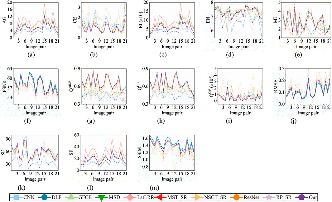
Figure 4. Metrics of all 21 image pairs. The data of the first 9 methods are from the workbench in reference [22]. The best result and our result are bolded, and there is one bolded result if our result is the best. (a) AG (b) CE (c) EI (d) EN (e) MI (f) PSNR (g) Q^AB/F (h) Q^CB (i) Q^CV (j) RMSE (k) SD (l) SF (m) SSIM.

Table 2

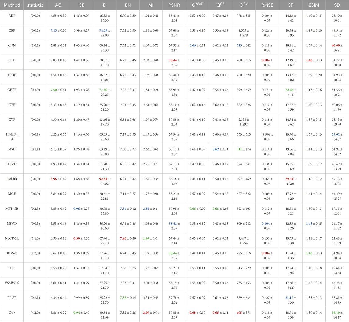
Table 2. Different methods’ average results of metrics on VIFB dataset. Red, green, and blue denote the best, second best, and third best results, numbers in the second column brackets are the statistical result of the best, second best, and third best results correspondingly. Some red, green, and blue results are ranked according to the third decimal place. Considering the size of the table, all results are only reserved for two decimal places. Considering the size of table, all results are only reserved for two decimal places. The data of the first 20 methods are from the workbench in [22].

Additionally, Figure 5 shows the fused image on the man Car image pair. Our method preserves as much information as possible: the majority of details from the visible and infrared image can be found in the fused image. In contrast, there are some notable discontinuities in NSCT_SR, which results in the introduction of certain new features and the loss of some crucial information. While DLF, MSD, and ResNet save more information about visible image, CNN, LatLRR, and GFCE store more information about the infrared image. The results of RP_SR and MST_SR are comparatively close to our method. It is possible to include some artificial features because the dictionary of sparse representation is fixed. Both colors of the car’s rear door and the roof adjacent to it have altered, as we can see in Figure 5k. There are some pink zones on the ground in Figures 5h,k, they are not present in the source image pair. In contrast, our method effectively suppresses the artificial features, as Figure 5l shows. This demonstrates once more the advantages of our method in terms of maintaining image information and suppressing artificial features. Figures 5c,d,j show that the overall images are smooth and the fused images are close to the source image pairs, but some details are not well preserved. The white zone beside the car is unobtrusive in Figures 5d,j, it is also hard to observe the trees in front of the farthest house. This indicates that DLF and RestNet lose more details while they capture more structural information; this is consistent with the metric results.

Figure 5

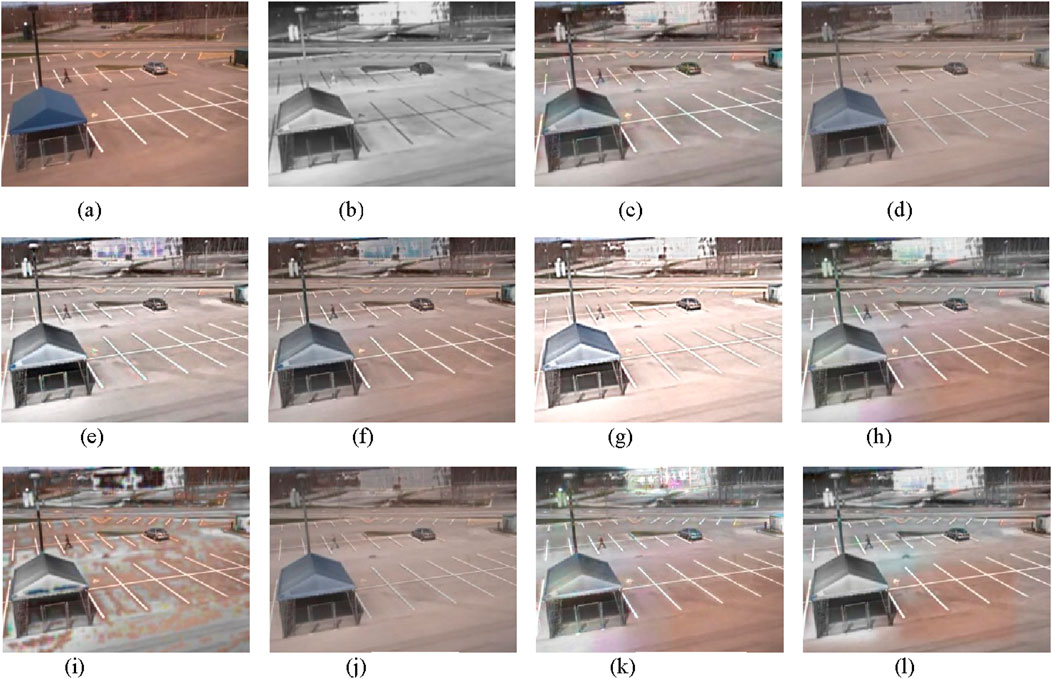
Figure 5. The visible and infrared image fusion result on the manCar image pair. The results of the first 9 methods are from the workbench in reference [22]. (a) Visible (b) Infrared (c) CNN (d) DLF (e) GFCE (f) MSD (g) LatLRR (h) MST_SR (i) NSCT_SR (j) ResNet (k) RP_SR (l) Our.

4.3 Experiment results on TNO dataset

We carried out another experiment on the TNO dataset to further examine the performance of our method; only nine methods that performed well on the VIFB dataset are compared in this experiment. The results of metrics are listed in Table 3. Our method receives three best, 2 seconds, one-third, and outperforms the others. It is easy to find that the advantages remain in information theory-based metrics, image feature-based metrics, and human visual perception, which is consistent with the results on the VIFB dataset. The performance of Q^CV declines compared with the results on the VIFB dataset. But our method continues to perform better in Q^CB; both Q^CB and Q^CV belong to human visual perception metrics, so we can still believe that our method has good ability to capture the major features in the human visual system. RMSE and SSIM are not prominent, this phenomenon can also be observed in other superior methods, including CNN, GFCE, LatLRR, RP_SR, and MST_SR. DLF and ResNet still obtain the best results in RMSE and SSIM. According to the STDs, smaller values are observed for the CE, EN, PSNR, RMSE, SSIM, and SD metrics, slightly poorer performance is seen for the MI and Q^CB metrics, and the remaining metrics exhibit performances close to the average level.

Table 3

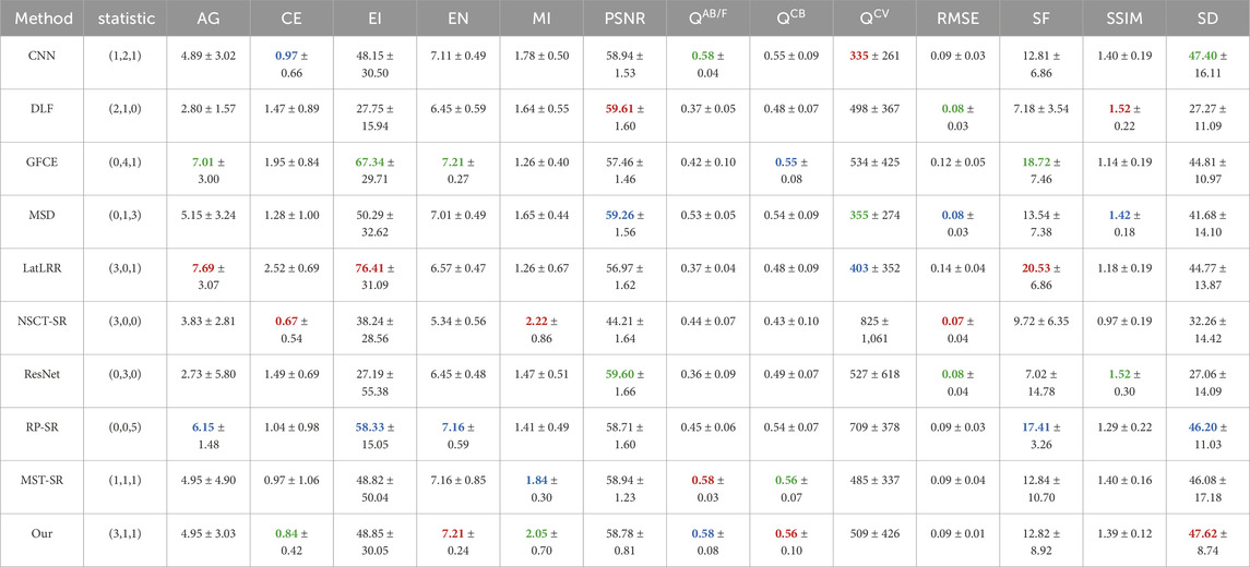
Table 3. Different methods’ average results of metrics on the TNO dataset. Red, green, and blue mean the best, second best, and third best results, numbers in the second column brackets are the statistical result of the best, second best, and third best results correspondingly. Some red, green, and blue results are ranked according to the third decimal place. Considering the size of table, all results are only reserved for two decimal places.

Furthermore, Figure 6 displays the metrics of 20 image pairs that were selected at random from the TNO dataset. The metrics of several image pairs also varied significantly from one another. Overall, our method performs better in CE, EN, Q^CB, and SD, as Figures 6b,d,h,k show. Even though our method’s average CE in Table 3 is not the best, it outperforms NSCT_SR in more image pairs, which proves the stability of our method. Additionally, our method’s performance is extremely close to the best ones in PSNR, Q^AB/F, Q^CV, RMSE, and SSIM, as Figures 6f,g,i,j,m show, while our method’s performance is mediocre in AG, EI, and SF.

Figure 6

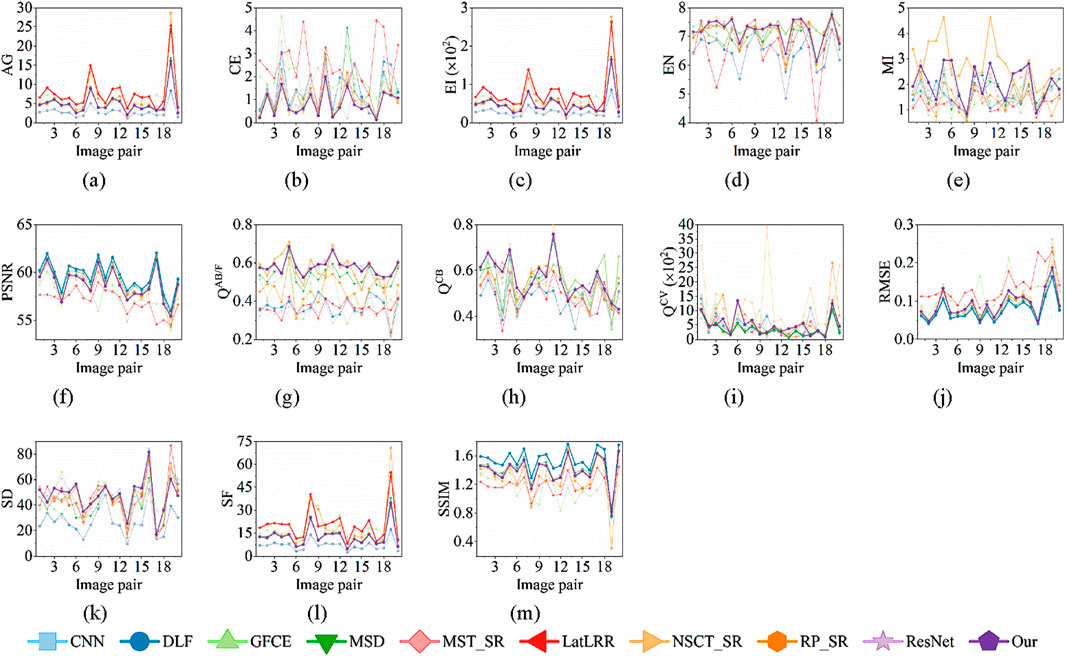
Figure 6. Metrics of 20 randomly selected image pairs. The best result and our result are bolded, and there is one bolded result if our result is the best. (a) AG (b) CE (c) EI (d) EN (e) MI (f) PSNR (g) Q^AB/F (h) Q^CB (i) Q^CV (j) RMSE (k) SD (l) SF (m) SSIM.

Figure 7 displays the fused images of different methods on the 29-th image pair. There are still some discontinuities in NSCT_SR, as Figure 7b shows. In GFCE and RP_SR, there are several unexpected new features about the window, as Figures 7e,j show. DLF and RestNet contain more information than the infrared image and the bright message in the sky is lost, as Figures 7d,i show. DLF and RP_SR lose some details about the letter box, as Figures 7d,i show. MSD and LatLRR save more information about the cloud and the visible and infrared features are very clear. Our method only contains a little of the cloud features of the visible image, but the dark and bright feature of the sky is retained more, as Figure 7l shows.

Figure 7

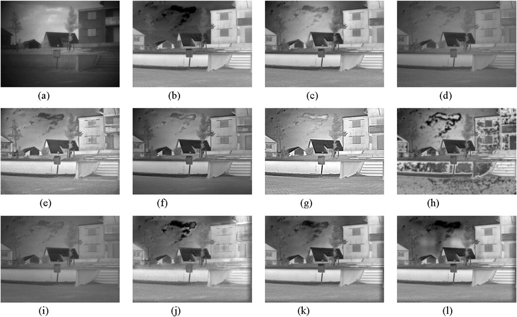
Figure 7. The visible and infrared image fusion result on the 29-th image pair. (a) Visible (b) Infrared (c) CNN (d) DLF (e) GFCE (f) Hybrid_MSD (g) LatLRR (h)NSCT_SR (i) ResNet (j) RP_SR (k) MST_SR (l) Our.

4.4 Experiment results on the LLVIP dataset

In order to further investigate the performance of our method, we conducted another experiment on the LLVIP dataset; the same methods that were used on TNO dataset are compared in this experiment. The image pairs from the LLVIP dataset are captured in a very dark environment. Table 3 lists the results of the metrics, our method receives one best and 3 seconds. Although there are fewer top three metric results, it is worth noting that the metric results of our method are very close to the better ones. Overall, LatLRR obtains the better scores. DLF and ResNet still share good results with RMSE and SSIM while the other metric results are not outstanding. According to the STDs, smaller values are observed for the Q^AB/F, RMSE, and SF metrics, slightly poorer performance is seen for the EN, PSNR and SD metrics, while the remaining metrics exhibit performances close to the average level. The assessment scores for the fusion results of all methods exhibit significant fluctuations across different image data sets, due mainly to various degrees of statistical complexities amongst the data sets. However, it is observed that the performance of the proposed algorithm exhibits relatively smaller fluctuations across most evaluation metrics, as indicated by the smaller standard deviations in Tables 2–4, indicative of the better stability in our proposed method.

Table 4

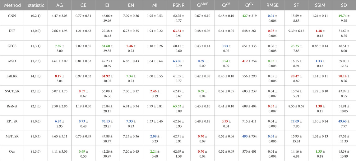
Table 4. Different methods’ average results of metrics on the LLVIP dataset. Red, green, and blue mean the best, second best, and third best results, numbers in the second column brackets are the statistical result of the best, second best, and third best results correspondingly. Considering the size of table, all results are only reserved for two decimal places.

Additionally, Figure 8 shows the metrics of 20 image pairs selected at random from the LLVIP dataset. Our method yields the best outcome in Q^AB/F, as Figure 8g shows. As shown in Figures 8b,e,i,m, our method’s performance is nearly as good as the best in CE, MI, Q^CB, Q^CV, and SSIM. In AG, EI, EN, PSNR, RMSE, SD, and SF, our method performs mediocrely. LatLRR performs better overall in AG, EI, SD, and SF but exhibits subpar results in PSNR, RMSE, and Q^AB/F, as Figures 8f,g,j show. Our approach presents better balanced results in all metrics than LatLRR, despite a slight performance drop when compared to the VIFB and TNO datasets. DLF also shows better performance in PSNR, RMSE, and SSIM, but its performance is not exceptional in CE, EI, EN, Q^CB, and SD.

Figure 8

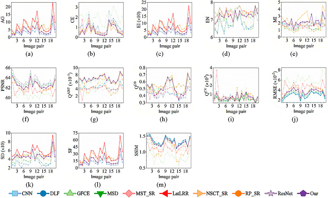
Figure 8. Metrics of 20 randomly selected image pairs. The best result and our result are bolded, and there is one bolded result if our result is the best. (a) AG (b) CE (c) EI (d) EN (e) MI (f) PSNR (g) Q^AB/F (h) Q^CB (i) Q^CV (j) RMSE (k) SD (l) SF (m) SSIM.

Figure 9 shows the selected fusion results on the 3-th image pair, which was taken in a very dim setting. It is easy to observe in Figure 9e that GFCE lost the dark information. The wall and pedestrians still have some noticeable discontinuities in NSCT_SR, and RP_SR also exhibits this problem. Due to the loss of some information from the visible source image, the words on the wall are not discernible in DLF and ResNet. The fusion performance is close in Figures 9c,f,g,k,l, CNN and LatLRR achieve superior results in motorbike light out of the five results. Our approach and MST_SR preserve more dark information while losing the visible source image’s bright light information.

Figure 9

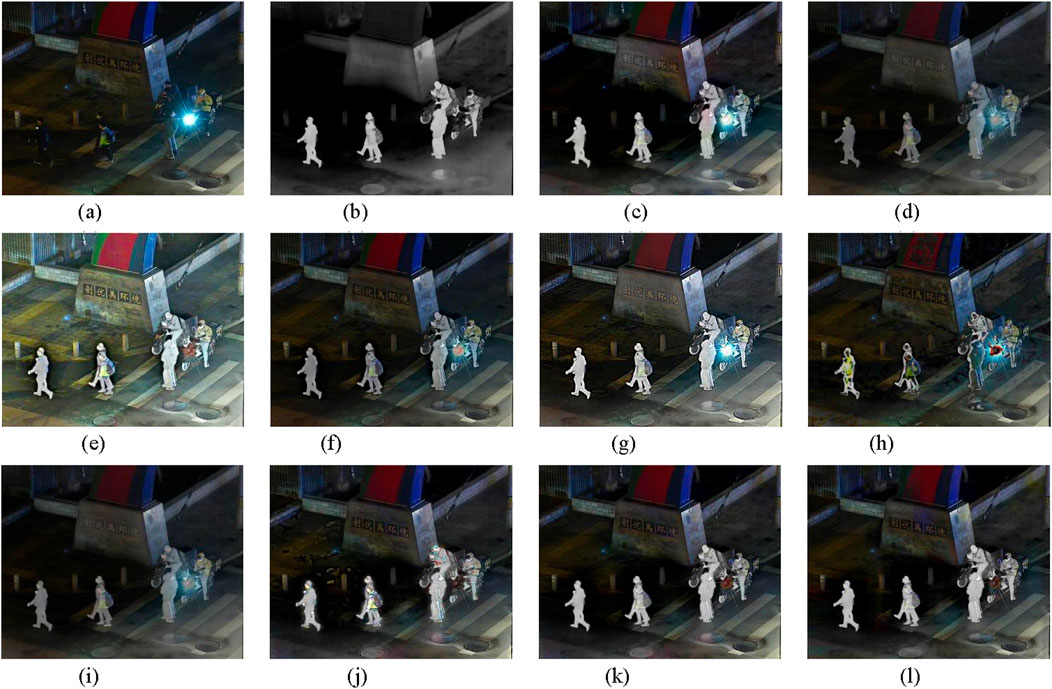
Figure 9. The visible and infrared image fusion results on the third image pair. (a) Visible (b) Infrared (c) CNN (d) DLF (e) GFCE (f) Hybrid_MSD (g) LatLRR (h) NSCT_SR (i) ResNet (j) RP_SR (k) MST_SR (l) Our.

4.5 Discussion

4.5.1 Runtime comparison

Table 5 lists the runtime of various algorithms on three datasets. It is evident that there are substantial differences in runtime across the various methods. ResNet performs better than other methods on VIFB and LLVIP datasets, while GFCE has a lower runtime cost on TNO dataset. NSCT_SR takes the longest on all three datasets, while LatLRR also needs to take a lengthy time to fuse a single image pair. Additionally, we can see that a particular method’s runtime varies greatly depending on the dataset; this is particularly true for LatLRR and NSCT_SR. The size of source image pairs from LLVIP are larger than those from the other two datasets. It theoretically takes more time on the LLVIP dataset. On the other hand, even though the size of the source image pairs from TNO are larger than that from VIFB, some algorithms, including DLF, GFCE, MSD, LatLRR, NSCT_SR, and RP_SR, have shorter runtimes on the TNO dataset. This is because different datasets have varying levels of complexity. When complexity is higher, feature extraction needs more time. Overall, GFCE and ResNet share computational efficiency. Our method’s runtime is comparable to that of DLF, MSD, RP_SR, and MST_SR. However, it can be observed that methods with notable advantages in runtime, such as ResNet and GFCE, perform far worse than the proposed method in image fusion. Conversely, methods that achieve comparable image fusion results to the proposed method, such as LatLRR and NSCT-SR, have a significantly higher time cost. As for MST-SR, although its time cost is slightly better than the proposed method on the VIFB and TNO datasets, its average time cost advantage is only 0.427 s, and its image fusion results across all datasets are far inferior to the proposed method. In conclusion, the proposed method, while maintaining an advantage in image fusion quality, also generally achieves improved runtime performance compared to methods with similar fusion quality.

Table 5

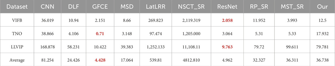
Table 5. The runtime of different methods in three datasets (seconds per image pair). Red is the best result.

Although LatLRR can obtain good fusion performance, the runtime cost is significantly expensive. NSCT_SR’s fusion performance is not exceptional and its runtime is lengthy. The aforementioned results lead us to the conclusion that there needs to be a compromise between fusion performance and runtime.

4.5.2 Analysis of parameter sensitivity

In order to analyze the parameter sensitivity of our method, both α and λ in Equation 4 are set among a discrete set {1e⁻⁷, 1e⁻⁶, 1e⁻⁵, 1e⁻⁴, 1e⁻³, 1e⁻², 1e⁻¹, 1, 10, 100}, and the results of 13 metrics are shown in Figure 10. The smaller the value, the better the result for three metrics: CE, Q^CV, and RMSE. When α and λ are in the range of 1e⁻⁷ to 10, the three metrics remain small and stable. Meanwhile, other metrics hold a high level. This illustrates that our method has good robustness, and it is easy to find a parameter pair that results in good performance. In addition, there are several noteworthy results. Firstly, the metrics, including AG, EI, EN, MI, Q^CB, SF, SD, CE, and Q^CV, improve when α is set to 100. However, PSNR is lower. Therefore, α cannot exceed 10 for overall performance, as Figure 10f shows. Second, RMSE does not change with the variation of parameters and always maintains a modest value; this proves that our sparse low-rank representation can be well implemented, and the error of image reconstruction is very close to zero. Third, SSIM improves when λ surpasses 10, but other metrics worsen. Therefore, λ cannot exceed 10 for overall performance.

Figure 10

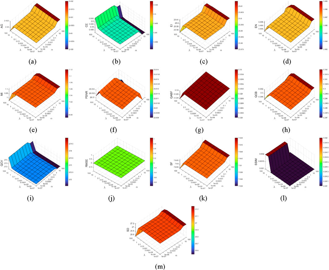
Figure 10. Analysis of parameter sensitivity. (a) AG (b) CE↓ (c) EI (d) EN (e) MI (f) PSNR (g) Q^AB/F (h) Q^CB (i) Q^CV↓ (j) RMSE↓ (k) SF (l) SSIM (m) SD.

In order to analyze the influence of decomposition levels, we set it in the discrete set {2, 3, 4, 5, 6, 7} and the results of different metrics are shown in Figure 11. When the decomposition levels increase, there are generally three types of change trends: increasing, decreasing, and first increasing then decreasing. Metrics, including CE, PSNR and Q^AB/F, show the increasing trend and maintain good results when the decomposition level is 4. As for AG, EI, EN, Q^CV, and RMSE, they decrease as the decomposition level is increasing. AG, EI, and EN receive the best results when the level is 2, while the value of Q^CV and RMSE are near the best result when the level exceeds 3. The rest of the metrics, including MI, Q^CB, SD, SF, and SSIM, show the trend of first increasing then decreasing. They obtain the best results when the decomposition level is 4. In conclusion, when the decomposition level is 4, metrics such as CE, MI, PSNR, Q^AB/F, Q^CB, Q^CV, RMSE, SD, SF, and SSIM, can obtain the best results or keep very near the best results while the other metrics still maintain relatively good results. Therefore, the decomposition level is recommended to be 4.

Figure 11

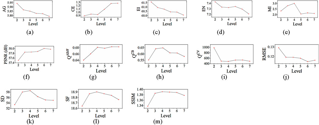
Figure 11. Influence of decomposition levels. (a) AG (b) CE↓ (c) EI (d) EN (e) MI (f) PSNR (g) Q^AB/F (h) Q^CB (i) Q^CV↓ (j) RMSE↓ (k) SD (l) SF (m) SSIM.

4.5.3 Effectiveness analysis of low-rank constraint

To further analyze the effectiveness of low-rank constraints in extracting image information, Figure 12 presents the visualization results of sparse coefficients and sparse low-rank coefficients. First, it can be observed that the number of nonzero elements in the sparse coefficients is relatively small, with larger magnitude values. This indicates that, in the sparse representation of infrared and visible images, greater weight is assigned to key features, while some detailed features tend to be overlooked. In contrast, due to the presence of the low-rank constraint, the sparse low-rank coefficients contain more nonzero elements, with values an order of magnitude lower than those of the sparse coefficients. This suggests that the sparse low-rank representation can extract more image features compared to the sparse representation. Furthermore, since low-pass band fusion is performed based on the maximum L1-norm fusion rule, when an image contains numerous features, the fusion is influenced not only by a few key features but also by other features that play a decisive role. Therefore, in summary, compared to MST-SR, the proposed infrared and visible image fusion method based on sparse low-rank representation can retain key features while extracting more detailed features, thereby preserving as much information from the original images as possible in the fused image. This also explains why the proposed method performs well in both information theory-based metrics and image feature-based metrics, further validating that the introduced low-rank constraint effectively enhances the quality of infrared and visible image fusion.

Figure 12

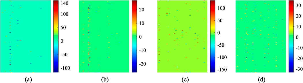
Figure 12. Coefficient visualization of the visible and infrared images. (a) SR coefficients of the visible image (b) SLR coefficients of the visible image (c) SR coefficients of the infrared image (d) SLR coefficients of the visible image.

5 Conclusion

In this paper, we combine sparse and low-rank constraints to present a novel visible and infrared image fusion method. Source images are firstly transformed into another domain to calculate their low-pass and high-pass bands by LP. Second, low-pass bands are represented with some sparse and low-rank coefficients. Then, specific fusion rules are adopted to fuse the low-pass and high-pass bands. Low-pass parts are a smooth version of source images; they are fused based on sparse low-rank representation. High-pass parts contain more details and the fusion is conducted based on the max-absolute rule. Finally, an inverse LP is conducted to obtain the fused image. Our method is validated on three public datasets. The results show that our method performs better in the three kinds of metrics: information theory-based, image feature-based, and human perception-based metrics. This means that low-rank constraints can effectively improve the performance of capturing details. Furthermore, our method obtains average performance in runtime cost and achieves relatively better balance between fusion performance and runtime cost. Our method also shows good parameter robustness; a good result can be obtained in a wide range of parameters.

Data availability statement

The VIFB dataset can be download from https://github.com/xingchenzhang/VIFB/tree/master (accessed on 17 June 2025). The TNO dataset can be download from https://figshare.com/articles/dataset/TNO_Image_Fusion_Dataset/1008029 (accessed on 17 June 2025). The LLVIP dataset can be download from https://bupt-ai-cz.github.io/LLVIP/ (accessed on 17 June 2025).

Author contributions

YZ: Writing – original draft, Data curation, Formal Analysis, Investigation, Methodology, Software, Validation. JW: Project administration, Resources, Supervision, Writing – review and editing. BY: Funding acquisition, Supervision, Writing – review and editing. HC: Methodology, Validation, Writing – review and editing. JF: Methodology, Writing – review and editing. ZW: Writing – review and editing. SY: Writing – review and editing.

Funding

The author(s) declare that financial support was received for the research and/or publication of this article. This research was funded by the Yunnan Provincial and Municipal Integration Special Project under Grant 202302AH360002 by the Young and Middle-Aged Academic and Technical Leaders Reserve Talents Project of Yunnan Province under Grant 202305AC160062 and by the Scientific Research Fund Project of Yunnan Provincial Department of Education under Grant 2024J0077.

Conflict of interest

Author JF was employed by Guangxi Huasheng new material Co., Ltd.

The remaining authors declare that the research was conducted in the absence of any commercial or financial relationships that could be construed as a potential conflict of interest.

Generative AI statement

The author(s) declare that no Generative AI was used in the creation of this manuscript.

Publisher’s note

All claims expressed in this article are solely those of the authors and do not necessarily represent those of their affiliated organizations, or those of the publisher, the editors and the reviewers. Any product that may be evaluated in this article, or claim that may be made by its manufacturer, is not guaranteed or endorsed by the publisher.

References

1. Zhang X. Benchmarking and comparing multi-exposure image fusion algorithms. Inf Fusion (2021) 74:111–31. doi:10.1016/j.inffus.2021.02.005

CrossRef Full Text | Google Scholar

2. Zhang Y, Zhang L, Bai X, Zhang L. Infrared and visual image fusion through infrared feature extraction and visual information preservation. Infrared Phys Technol (2017) 83:227–37. doi:10.1016/j.infrared.2017.05.007

CrossRef Full Text | Google Scholar

3. Bavirisetti D, Xiao G, Liu G. Multi-sensor image fusion based on fourth order partial differential equations. In: Proceedings of the 20th international conference information fusion. China: Xi’an (2017). p. 10–3.

Google Scholar

4. Ma J, Chen C, Li C, Huang J. Infrared and visible image fusion via gradient transfer and total variation minimization. Inf Fusion (2016) 31:100–9. doi:10.1016/j.inffus.2016.02.001

CrossRef Full Text | Google Scholar

5. Li H, Wu X. Infrared and visible image fusion using latent low-rank representation. arXiv preprint (2018). Available online at: https://arxiv.org/abs/1804.08992.

Google Scholar

6. Bavirisetti D, Dhuli R. Two-scale image fusion of visible and infrared images using saliency detection. Infrared Phys Technol (2016) 76:52–64. doi:10.1016/j.infrared.2016.01.009

CrossRef Full Text | Google Scholar

7. Bavirisetti D, Dhuli R. Fusion of infrared and visible sensor images based on anisotropic diffusion and karhunen-loeve transform. IEEE Sens J (2016) 16:203–9. doi:10.1109/jsen.2015.2478655

CrossRef Full Text | Google Scholar

8. Shreyamsha Kumar BK. Image fusion based on pixel significance using cross bilateral filter. Signal Image Video P (2013) 9:1193–204. doi:10.1007/s11760-013-0556-9

CrossRef Full Text | Google Scholar

9. Zhou Z, Dong M, Xie X, Gao Z. Fusion of infrared and visible images for night-vision context enhancement. Appl Opt (2016) 55:6480. doi:10.1364/ao.55.006480

PubMed Abstract | CrossRef Full Text | Google Scholar

10. Li S, Kang X, Hu J. Image fusion with guided filtering. IEEE Trans Image Process (2013) 22:2864–75. doi:10.1109/TIP.2013.2244222

PubMed Abstract | CrossRef Full Text | Google Scholar

11. Bavirisetti D, Xiao G, Zhao J, Dhuli R, Liu G. Multi-scale guided image and video fusion: a fast and efficient approach. Circuits Syst Signal Process (2019) 38:5576–605. doi:10.1007/s00034-019-01131-z

CrossRef Full Text | Google Scholar

12. Naidu V. Image fusion technique using multi-resolution singular value decomposition. Def Sci J (2011) 61:479. doi:10.14429/dsj.61.705

CrossRef Full Text | Google Scholar

13. Qi B, Bai X, Wu W, Zhang Y, Lv H, Li G. A novel saliency-based decomposition strategy for infrared and visible image fusion. Remote Sens. (2023) 15:2624. doi:10.3390/rs15102624

CrossRef Full Text | Google Scholar

14. Zhou Z, Wang B, Li S, Dong M. Perceptual fusion of infrared and visible images through a hybrid multi-scale decomposition with Gaussian and bilateral filters. Inf Fusion (2016) 30:15–26. doi:10.1016/j.inffus.2015.11.003

CrossRef Full Text | Google Scholar

15. Liu Y, Liu S, Wang Z. A general framework for image fusion based on multi-scale transform and sparse representation. Inf Fusion (2015) 24:147–64. doi:10.1016/j.inffus.2014.09.004

CrossRef Full Text | Google Scholar

16. Ma J, Zhou Z, Wang B, Zong H. Infrared and visible image fusion based on visual saliency map and weighted least square optimization. Infrared Phys Technol (2017) 82:8–17. doi:10.1016/j.infrared.2017.02.005

CrossRef Full Text | Google Scholar

17. Chen W, Miao L, Wang Y, Zhou Z, Qiao Y. Infrared–visible image fusion through feature-based decomposition and domain normalization. Remote Sens. (2024) 16:969. doi:10.3390/rs16060969

CrossRef Full Text | Google Scholar

18. Li L, Lv M, Jia Z, Jin Q, Liu M, Chen L, An effective infrared and visible image fusion approach via rolling guidance filtering and gradient saliency map. Remote Sens (2023) 15:2486. doi:10.3390/rs15102486

CrossRef Full Text | Google Scholar

19. Liu Y, Chen X, Cheng J, Peng H, Wang Z. Infrared and visible image fusion with convolutional neural networks. Int J Wavelets Multiresolut Inf Process (2018) 16:1850018. doi:10.1142/s0219691318500182

CrossRef Full Text | Google Scholar

20. Li H, Wu X, Kittler J. Infrared and visible image fusion using a deep learning framework. In: Proceedings of the 24th international conference on pattern recognition (ICPR). Beijing, China (2018). p. 20–4.

Google Scholar

21. Li H, Wu X, Durrani T. Infrared and visible image fusion with ResNet and zero-phase component analysis. Infrared Phys Technol (2019) 102. doi:10.1016/j.infrared.2019.103039

CrossRef Full Text | Google Scholar

22. Zhang X, Ye P, Xiao G. VIFB: a visible and infrared image fusion benchmark. In: Proceedings of the 2020 IEEE/CVF conference on computer vision and pattern recognition workshops (CVPRW). Seattle, WA, USA (2020).

Google Scholar

23. Wei Q, Liu Y, Jiang X, Su B, Yu M. DDFNet-A: attention-based dual-branch feature decomposition fusion network for infrared and visible image fusion. Remote Sens. (2024) 16:1795. doi:10.3390/rs16101795

CrossRef Full Text | Google Scholar

24. Xu Y, Fang X, Wu J, Li X, Zhang D. Discriminative transfer subspace learning via low-rank and sparse representation. IEEE Trans Image Process (2016) 25:850–63. doi:10.1109/tip.2015.2510498

PubMed Abstract | CrossRef Full Text | Google Scholar

25. Xue J, Zhao Y, Bu Y, Liao W, Chan J, Philips W. Spatial-spectral structured sparse low-rank representation for hyperspectral image super-resolution. IEEE Trans Image Process (2021) 30:3084–97. doi:10.1109/tip.2021.3058590

PubMed Abstract | CrossRef Full Text | Google Scholar

26. Donoho D. For most large underdetermined systems of linear equations the minimal l1-norm solution is also the sparsest solution. Commun. Pure Appl Math (2006) LIX:0797–829. doi:10.1002/cpa.20131

CrossRef Full Text | Google Scholar

27. Ahmed J, Gao B, Woo W, Zhu Y. Ensemble joint sparse low-rank matrix decomposition for thermography diagnosis system. IEEE Trans Ind Electron (2021) 68:2648–58. doi:10.1109/tie.2020.2975484

CrossRef Full Text | Google Scholar

28. Lin Z, Chen M, Ma Y. The augmented Lagrange multiplier method for exact recovery of corrupted low-rank matrices. arXiv:2011. arXiv: 1109.5055. doi:10.48550/arXiv.1009.5055

CrossRef Full Text | Google Scholar

29. Boyd S, Parikh N, Chu E, Peleato B, Eckstein J. Distributed optimization and statistical learning via the alternating direction method of multipliers. In: Now foundations and trends. Netherlands: Delft (2010). p. 1–122.

Google Scholar

30. Donoho DL. De-noising by soft-thresholding. IEEE Trans Inf Theor (1995) 41:613–27. doi:10.1109/18.382009

CrossRef Full Text | Google Scholar

31. Cai JF, Candès EJ, Shen ZW. A singular value thresholding algorithm for matrix completion. SIAM J Optimiz (2010) 20:1956–82. doi:10.1137/080738970

CrossRef Full Text | Google Scholar

32. Liu G, Lin Z, Yan S, Sun J, Yu Y, Ma Y. Robust recovery of subspace structures by low-rank representation. IEEE Trans Pattern Anal Mach Intell (2013) 35:171–84. doi:10.1109/tpami.2012.88

PubMed Abstract | CrossRef Full Text | Google Scholar

33. Li H, Manjunath B, Mitra S. Multisensor image fusion using the wavelet transform. Graph Models Image Process (1995) 57:235–45. doi:10.1006/gmip.1995.1022

CrossRef Full Text | Google Scholar

34. Toet A. The TNO multiband image data collection. Data Brief (2017) 15:249–51. doi:10.1016/j.dib.2017.09.038

PubMed Abstract | CrossRef Full Text | Google Scholar

35. Jia X, Zhu C, Li M, Tang W, Zhou W. LLVIP: a visible-infrared paired dataset for low-light vision. In: Proceedings of the 2021 IEEE/CVF international conference on computer vision workshops (ICCVW). Montreal: BC, Canada (2021).

Google Scholar