Inverse freeform design in non-imaging optics: Hamilton’s theory of geometrical optics, optimal transport, and least-squares solvers

We present a systematic derivation of three mathematical models of increasing complexity for optical design, based on Hamilton’s characteristic functions and conservation of luminous flux, and briefly explain the connection with the mathematical theory of optimal transport. We outline several iterative least-squares solvers for our models and demonstrate their performance for a few challenging problems.

1 Introduction

Nowadays, traditional incandescent light bulbs have largely been replaced by LED lamps, mainly because LEDs are highly energy efficient and last for long duration. However, to create a desired light output with LEDs, optical systems are required. Therefore, in the illumination optics industry, a lot of research is carried out on the design of optical systems for a myriad of applications.

The industry standard in optical design is (quasi-)Monte Carlo ray tracing. These are forward methods, which compute the target light distribution for a given source, typically LED, and a given optical system, tracing a large collection of rays from the source to target. Convergence of ray tracing is slow and requires millions or, maybe, even billions of rays to accurately compute the target distribution; see ([1], Chapter3). Moreover, to realize the desired target distribution, these methods have to be embedded in an iterative procedure, adjusting system parameters. More specifically to update these parameters, sophisticated design methods combine an iterative gradient-based optimization method, to minimize a suitably chosen merit function, with differentiable ray tracing to compute the required gradient. These methods are efficient and broadly applicable; see e.g., [31, 32]

A promising alternative are inverse methods. These methods compute the shape/location of the optical surface(s) in one go, given a source distribution and a desired target distribution. The surfaces are referred to as freeform since they have no imposed symmetries. Mathematical models for inverse methods are based on the principles of geometrical optics and conservation of luminous flux. Our models contain the following: a geometrical equation describing the shape/location of the optical surface(s), an (implicit) relation between the location of an optical surface and the optical map, which expresses target coordinates as a function of source coordinates, a matrix equation for the optical map, a conservation law of luminous flux, and a constraint on the luminous flux. The geometrical equation can be derived evaluating one of Hamilton’s characteristic functions and has multiple solutions. The optical map satisfies the luminous flux balance, which is a Jacobian equation, and a matrix equation, which has to be supplemented with the unconventional transport boundary condition. Our models are restricted to zero-étendue sources; more specifically, we consider only planar sources emitting a parallel beam of light or point sources.

In mathematics, the abstract theory of optimal transport is the correct framework to formulate optical design problems. The subject of optimal transport theory is to compute a transport plan (mapping) that transforms a given density function into another one, minimizing the transportation cost and subject to a(n) (integral) conservation law; see [2]. One of the governing equations is precisely the geometrical equation, containing a so-called cost function in the right hand side. The transportation cost is then a cost functional (an integral of the cost function). The analogy with optical design is obvious, the two density functions correspond to the source and target distributions, the transport plan to the optical map, the cost functional can be associated with the optical path length, and the conservation law applies to the luminous flux.

Based on the analogy with optimal transport theory, we can distinguish three mathematical models of increasing complexity. First, in the simplest model, the geometrical equation contains a quadratic cost function, and the Jacobian equation reduces to the standard Monge–Ampère (MA) equation, which is a second-order, non-linear, elliptic partial differential equation (PDE) [3], defining the location of an optical surface. In the next model, the cost function is no longer quadratic and the Jacobian equation corresponds to a generalized Monge–Ampère (GMA) equation. Finally, the most complicated model does not allow a description in terms of a cost function anymore; instead, a so-called generating function is required. The Jacobian equation now corresponds to a generated Jacobian (GJ) equation.

The procedure to derive our mathematical models consists of the following steps:

1. By applying principles of geometrical optics, derive the geometrical equation.

2. Formulate the luminous flux balance, which is a Jacobian equation for the optical map.

3. Based on optimal transport theory, select a uniquely defined solution from the geometrical equation.

4. Derive the necessary (zero-gradient) condition for this solution to define a unique relation between the location of an optical surface and the optical map.

5. Derive from the zero-gradient condition the matrix equation for the Jacobi matrix of the optical map.

6. Combine the luminous flux balance with the matrix equation to derive a constraint on the luminous flux.

There are many numerical methods available for inverse freeform optical design; for a detailed survey, see [4], Chapter 5. Without trying to be complete, a possible categorization is as follows: first, numerical methods for (G)MA equations governing the shape/location of an optical surface; second, optimization methods; third, geometrical construction methods; and fourth, ray mapping methods. In the first category are methods that directly solve the second-order PDE of MA type by discretization and subsequent iteration for the resulting algebraic system. Examples of these are reported in papers by Froese [5], using a wide-stencil finite difference scheme, Benamou et al. [6], using finite differences, Brix et al. [35], using B-spline collocation, and Kawecki et al. [7], using finite elements, to just name a few examples. Methods in the second category are based on optimal transport theory and determine the optical surface(s) by minimizing the cost functional subject to conservation of luminous flux, see, e.g., [33, 34] Next, based on the work of Caffarelli and Oliker [8], geometrical construction methods for optical surfaces with paraboloids have been investigated by Kitagawa et al. [9] and Mérigot and Thibert [10] for the GMA equation, and by Galouët et al. [11] for the GJ equation. Finally, in ray mapping methods, the computation of the optical surface(s) is split into two parts, i.e., first, an estimate of the optical map is computed from an optimal transport problem, and subsequently, the optical surface is computed employing the law of reflection/refraction; see e.g., [36–38]

Our methods are of the first category. The publication that inspired us to develop our numerical solvers is by Caboussat et al. [12]. In this paper, the authors present a least-squares method to solve the Dirichlet problem for the standard MA equation. Prins adjusted their method to include the transport boundary condition; see [13]. In a series of papers, Yadav and Romijn extended the method for the GMA equation, corresponding to a non-quadratic cost function; see [14], [15, 16]. Romijn further extended our least-squares methods to deal with the GJ equation; see [17, 18]. Specifically, for the cost function models, we have developed a two-stage algorithm, i.e., we first compute the optical map and subsequently the shape/location of the optical surface(s). For both stages, we apply a least-squares method. For the generating function model, the optical map and the optical surface(s) have to be computed simultaneously, also in a least-squares fashion.

In this paper, we present a systematic derivation of all models and outline numerical simulation methods. The content is then as follows. First, in Section 2, we introduce Hamilton’s characteristic functions needed to derive the geometrical equations. In Section 3, we give an outline of optimal transport theory, needed to select a uniquely defined solution of the geometrical equation. A generic conservation law for luminous flux is presented in Section 4. Next, in Section 5, we apply the results of the previous sections to present a hierarchy of models based on three example systems. A concise description of our numerical methods is presented in Section 6. To demonstrate the performance of our methods, we present a few challenging examples in Section 7. Concluding remarks are given in Section 8, and the paper is concluded with a nomenclature list.

2 Hamilton’s characteristic functions

In this section, we introduce Hamilton’s characteristic functions which are needed for the derivation of the geometrical equations in Section 5; see, e.g., [19], pp. 94–107; [20], Section 4.1 for a more detailed account. Our starting point is the eikonal equation given by

$|\nabla \phi |=n,(1)$

where $\phi =\phi (\underline{\mathit{r}})$ is the phase of an electromagnetic wave and $n=n(\underline{\mathit{r}})$ is the refractive index field as functions of the (three-dimensional) position vector (or coordinates) $\underline{\mathit{r}}\in {\mathbb{R}}^3$ of a typical point. A surface $\phi (\underline{\mathit{r}})=\mathrm{C}\mathrm{o}\mathrm{n}\mathrm{s}\mathrm{t}$ is a wavefront. We denote three-dimensional vectors in bold font with an underbar $\left(\underline{}\right)$ , to distinguish them from two-dimensional vectors, which are only written in bold font. Equation 1 describes free propagation of light waves and no longer holds when a light wave is reflected or refracted at an optical surface. The eikonal Equation 1 is a first-order non-linear PDE, which has the characteristic strip equations

$\frac{\mathrm{d}\underline{\mathit{r}}}{\mathrm{d}s}=\frac{1}{n}\nabla \phi ,\frac{\mathrm{d}\phi }{\mathrm{d}s}=n,\frac{\mathrm{d}}{\mathrm{d}s}\left(\nabla \phi \right)=\nabla n.(2)$

See, e.g., Kevorkian [21]. The curves $\mathcal{C}:\underline{\mathit{r}}=\underline{\mathit{r}}(s)$ , parameterized by the arc length $s$ , are the characteristics of (1). The system of ordinary differential equations in (2) determines the location of the characteristics and the solution along the characteristics, from which the solution of (1) can be reconstructed. From the first equation in (2), we conclude that the characteristics are orthogonal trajectories to the wavefronts, i.e., characteristics are light rays; see, e.g., [20], p. 114.

Hamilton’s characteristic functions are related to the optical path length of a ray, which we, therefore, introduce next. We assume that $n(\underline{\mathit{r}})$ is piecewise continuous, with jumps at lens surfaces; consequently, rays are continuous and consist of piecewise differentiable curve segments; cf. Equation 2. In this setting, we define the optical path length (OPL) between the points ${\mathrm{P}}_1$ (position vector $\underline{\mathit{r}}={\underline{\mathit{r}}}_1$ ) and ${\mathrm{P}}_2$ (position vector $\underline{\mathit{r}}={\underline{\mathit{r}}}_2$ ), connected by a light ray along the curve $\mathcal{C}$ , as

$\left[{\mathrm{P}}_1,{\mathrm{P}}_2\right]=d_{\text{opt}}\left({\underline{\mathit{r}}}_1,{\underline{\mathit{r}}}_2\right)≔{\int }_{\mathcal{C}}n\left(\underline{\mathit{r}}\left(s\right)\right)\mathrm{d}s.(3)$

A consequence of Fermat’s principle is that the optical path length $[{\mathrm{P}}_1,{\mathrm{P}}_2]$ is stationary with respect to variations in the curve $\mathcal{C}$ ; see, e.g., [20], p. 740.

Consider an optical system consisting of a source, located in a plane $z=z_{\mathrm{s}}$ (source plane), emitting light which via a sequence of reflectors and/or lenses arrives at a plane $z=z_{\mathrm{t}}$ (target plane). The $z$ -axis is referred to as the optical axis. In this paper, we use the subscripts $\mathrm{s}$ and $\mathrm{t}$ for variables/vectors to denote their value at the source and target, respectively. Let $\widehat{\underline{\mathit{v}}}={(v_1{v}_2{v}_3)}^{\mathrm{T}}=\mathrm{d}\underline{\mathit{r}}/\mathrm{d}s$ denote the unit tangent vector of a ray; thus, $\nabla \phi =n\widehat{\underline{\mathit{v}}}$ ; cf. Equation 2. Unit vectors are denoted with a hat $(\widehat{})$ . Let ${\mathrm{Q}}_{\mathrm{s}}$ (position vector $\underline{\mathit{r}}={\underline{\mathit{r}}}_{\mathrm{s}}$ ) and ${\mathrm{Q}}_{\mathrm{t}}$ (position vector $\underline{\mathit{r}}={\underline{\mathit{r}}}_{\mathrm{t}}$ ) be two points on the source and target plane, respectively; then, from Equation 3, we obtain

$\left[{\mathrm{Q}}_{\mathrm{s}},{\mathrm{Q}}_{\mathrm{t}}\right]=d_{\text{opt}}\left({\underline{\mathit{r}}}_{\mathrm{s}},{\underline{\mathit{r}}}_{\mathrm{t}}\right)={\int }_{\mathcal{C}}n\widehat{\underline{\mathit{v}}}\cdot \widehat{\underline{\mathit{v}}}\mathrm{d}s={\int }_{\mathcal{C}}\nabla \phi \cdot \mathrm{d}\underline{\mathit{r}}=\phi \left({\underline{\mathit{r}}}_{\mathrm{t}}\right)-\phi \left({\underline{\mathit{r}}}_{\mathrm{s}}\right).(4)$

Note that reversing the direction of integration yields the symmetry property of $d_{\text{opt}}$ , i.e.,

$\begin{array}{cc}\hfill d_{\text{opt}}\left({\underline{\mathit{r}}}_{\mathrm{t}},{\underline{\mathit{r}}}_{\mathrm{s}}\right)& ={\int }_{-\mathcal{C}}\left(-n\widehat{\underline{\mathit{v}}}\right)\cdot \left(-\widehat{\underline{\mathit{v}}}\right)\mathrm{d}s\hfill \\ \hfill & ={\int }_{-\mathcal{C}}-\nabla \phi \cdot \mathrm{d}\underline{\mathit{r}}\hfill \\ \hfill & =-\phi \left({\underline{\mathit{r}}}_{\mathrm{s}}\right)+\phi \left({\underline{\mathit{r}}}_{\mathrm{t}}\right)\hfill \\ \hfill & =d_{\text{opt}}\left({\underline{\mathit{r}}}_{\mathrm{s}},{\underline{\mathit{r}}}_{\mathrm{t}}\right)\hfill \end{array}(5)$

as one would expect from the definition in Equation 3. Observe that $d_{\text{opt}}$ is a metric since $d_{\text{opt}}({\underline{\mathit{r}}}_{\mathrm{s}},{\underline{\mathit{r}}}_{\mathrm{t}})\ge 0$ , with equality only if ${\underline{\mathit{r}}}_{\mathrm{s}}={\underline{\mathit{r}}}_{\mathrm{t}}$ , and it satisfies the triangle inequality due to Fermat’s principle. The symmetry of $d_{\text{opt}}$ is stated in Equation 5.

For ease of presentation, we use the shorthand notation ${\widehat{\underline{\mathit{v}}}}_{\mathrm{s}}=\widehat{\underline{\mathit{s}}}$ and ${\widehat{\underline{\mathit{v}}}}_{\mathrm{t}}=\widehat{\underline{\mathit{t}}}$ . Straightforward differentiation of the expression for $d_{\text{opt}}({\underline{\mathit{r}}}_{\mathrm{s}},{\underline{\mathit{r}}}_{\mathrm{t}})$ in Equation 4 gives

${\nabla }_{\mathrm{s}}{d}_{\text{opt}}\left({\underline{\mathit{r}}}_{\mathrm{s}},{\underline{\mathit{r}}}_{\mathrm{t}}\right)=-\nabla \phi \left({\underline{\mathit{r}}}_{\mathrm{s}}\right)=-n_{\mathrm{s}}\widehat{\underline{\mathit{s}}},{\nabla }_{\mathrm{t}}{d}_{\text{opt}}\left({\underline{\mathit{r}}}_{\mathrm{s}},{\underline{\mathit{r}}}_{\mathrm{t}}\right)=\nabla \phi \left({\underline{\mathit{r}}}_{\mathrm{t}}\right)=n_{\mathrm{t}}\widehat{\underline{\mathit{t}}},(6)$

where ${\nabla }_{\mathrm{s}}$ denotes the gradient with respect to the source coordinates ${\underline{\mathit{r}}}_{\mathrm{s}}$ and likewise for ${\nabla }_{\mathrm{t}}$ . From these relations, we readily conclude that

$|{\nabla }_{\mathrm{s}}{d}_{\text{opt}}|=n_{\mathrm{s}},|{\nabla }_{\mathrm{t}}{d}_{\text{opt}}|=n_{\mathrm{t}},$

i.e., $d_{\text{opt}}$ satisfies the eikonal equation in both source and target coordinates.

A ray is completely determined by its position and direction coordinates. Position coordinates $\mathit{q}\in {\mathbb{R}}^2$ are defined as the projection on a plane $z=\mathrm{C}\mathrm{o}\mathrm{n}\mathrm{s}\mathrm{t}$ of the position vector $\underline{\mathit{r}}$ of a typical point on the ray. Position coordinates in the source and target planes are denoted by ${\mathit{q}}_{\mathrm{s}}$ and ${\mathit{q}}_{\mathrm{t}}$ , respectively. Thus, ${\mathrm{Q}}_{\mathrm{s}}$ , with position vector ${\underline{\mathit{r}}}_{\mathrm{s}}=({\mathit{q}}_{\mathrm{s}},z_{\mathrm{s}})$ , will denote the point at which a light ray is emitted from the source plane, and ${\mathrm{Q}}_{\mathrm{t}}$ , with the position vector ${\underline{\mathit{r}}}_{\mathrm{t}}=({\mathit{q}}_{\mathrm{t}},z_{\mathrm{t}})$ , as the point at which it arrives at the target plane. Next, selecting the first two components from the equation $n\frac{\mathrm{d}\underline{\mathit{r}}}{\mathrm{d}s}=n\widehat{\underline{\mathit{v}}}=\nabla \phi$ , we introduce the momentum vector $\mathit{p}\in {\mathbb{R}}^2$ as

$\mathit{p}≔n\frac{\mathrm{d}\mathit{q}}{\mathrm{d}s}=n\left(\begin{array}{c}\hfill v_1\hfill \\ \hfill v_2\hfill \end{array}\right)=\left(\begin{array}{c}\hfill \frac{\partial \phi }{\partial q_1}\hfill \\ \hfill \frac{\partial \phi }{\partial q_2}\hfill \end{array}\right)≕\frac{\partial \phi }{\partial \mathit{q}}.(7)$

Thus, the momentum vector is the projection of $\nabla \phi (\mathit{x})$ on a plane $z=\mathrm{C}\mathrm{o}\mathrm{n}\mathrm{s}\mathrm{t}$ and determines the direction of a light ray. Momentum vectors at the source and target are denoted with ${\mathit{p}}_{\mathrm{s}}$ and ${\mathit{p}}_{\mathrm{t}}$ , respectively. The variables $\mathit{q}=\mathit{q}(z)$ and $\mathit{p}=\mathit{p}(z)$ are referred to as phase-space coordinates and together constitute phase space.

In the remainder of this paper, we assume that $n(\underline{\mathit{r}})$ is piecewise constant, with possible discontinuities at optical interfaces, and consequently, a light ray consists of piecewise straight line segments. Below, we define four characteristic functions which relate the optical path length to phase-space coordinates at the source and target.

Point characteristic

As a function of the position coordinates ${\mathit{q}}_{\mathrm{s}}$ and ${\mathit{q}}_{\mathrm{t}}$ , the point characteristic $V$ is the optical path length of the ray connecting the points ${\mathrm{Q}}_{\mathrm{s}}$ and ${\mathrm{Q}}_{\mathrm{t}}$ , i.e.,

$V\left({\mathit{q}}_{\mathrm{s}},{\mathit{q}}_{\mathrm{t}}\right)≔d_{\text{opt}}\left(\left({\mathit{q}}_{\mathrm{s}},z_{\mathrm{s}}\right),\left({\mathit{q}}_{\mathrm{t}},z_{\mathrm{t}}\right)\right)=\left[{\mathrm{Q}}_{\mathrm{s}},{\mathrm{Q}}_{\mathrm{t}}\right].(8)$

From Equation 4, we conclude that $V({\mathit{q}}_{\mathrm{s}},{\mathit{q}}_{\mathrm{t}})=\phi ({\mathit{q}}_{\mathrm{t}},z_{\mathrm{t}})-\phi ({\mathit{q}}_{\mathrm{s}},z_{\mathrm{s}})$ . Combining this relation with the equations in Equation 6, selecting the first two components in both equations, we find for the directional derivatives $\frac{\partial V}{\partial {\mathit{q}}_{\mathrm{s}}}$ and $\frac{\partial V}{\partial {\mathit{q}}_{\mathrm{t}}}$ the following expressions:

$\frac{\partial V}{\partial {\mathit{q}}_{\mathrm{s}}}=-n_{\mathrm{s}}\left(\begin{array}{c}\hfill s_1\hfill \\ \hfill s_2\hfill \end{array}\right)=-{\mathit{p}}_{\mathrm{s}},\frac{\partial V}{\partial {\mathit{q}}_{\mathrm{t}}}=n_{\mathrm{t}}\left(\begin{array}{c}\hfill t_1\hfill \\ \hfill t_2\hfill \end{array}\right)={\mathit{p}}_{\mathrm{t}};(9)$

cf. Equation 7. Typically, Equations 8, 9 are used to derive a geometrical equation for optical systems described in terms of the position coordinates ${\mathit{q}}_{\mathrm{s}}$ and ${\mathit{q}}_{\mathrm{t}}$ . An example is the parallel-to-near-field reflector, discussed in Section 5.3.

Mixed characteristic of the first kind

Let a light ray connect the points ${\mathrm{Q}}_{\mathrm{s}}({\mathit{q}}_{\mathrm{s}},z_{\mathrm{s}})$ and ${\mathrm{Q}}_{\mathrm{t}}({\mathit{q}}_{\mathrm{t}},z_{\mathrm{t}})$ with momentum ${\mathit{p}}_{\mathrm{s}}$ and ${\mathit{p}}_{\mathrm{t}}$ , respectively; then, the mixed characteristic of the first kind $W$ is defined as

$W\left({\mathit{q}}_{\mathrm{s}},{\mathit{p}}_{\mathrm{t}}\right)≔V\left({\mathit{q}}_{\mathrm{s}},{\mathit{q}}_{\mathrm{t}}\right)-{\mathit{q}}_{\mathrm{t}}\cdot {\mathit{p}}_{\mathrm{t}}.(10)$

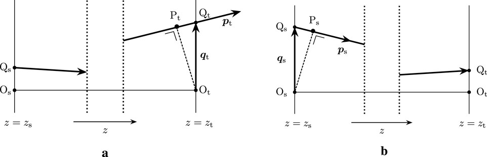
Straightforward differentiation yields $\partial W/\partial {\mathit{p}}_{\mathrm{s}}=\mathbf{0}$ and $\partial W/\partial {\mathit{q}}_{\mathrm{t}}=\partial V/\partial {\mathit{q}}_{\mathrm{t}}-{\mathit{p}}_{\mathrm{t}}=\mathbf{0}$ ; cf. Equation 9, second relation. Consequently, $W=W({\mathit{q}}_{\mathrm{s}},{\mathit{p}}_{\mathrm{t}})$ indeed. Moreover, we readily verify that

$\frac{\partial W}{\partial {\mathit{q}}_{\mathrm{s}}}=-{\mathit{p}}_{\mathrm{s}},\frac{\partial W}{\partial {\mathit{p}}_{\mathrm{t}}}=-{\mathit{q}}_{\mathrm{t}}.$

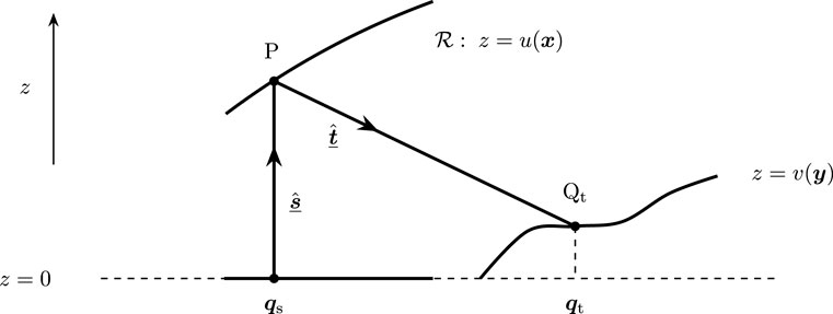
$W$ can be interpreted as a modification of $[{\mathrm{Q}}_{\mathrm{s}},{\mathrm{Q}}_{\mathrm{t}}]$ , which we show as follows. Assume that $z_{\mathrm{t}}>z_{\mathrm{s}}$ and define the point ${\mathrm{P}}_{\mathrm{t}}$ as the intersection of the ray segment arriving at ${\mathrm{Q}}_{\mathrm{t}}$ , parameterized by $\underline{\mathit{r}}(\lambda )={\underline{\mathit{r}}}_{\mathrm{t}}+\lambda \widehat{\underline{\mathit{t}}}$ , and the plane passing through the origin ${\mathrm{O}}_{\mathrm{t}}(\mathit{0},z_{\mathrm{t}})$ of the target plane (position vector ${\underline{\mathit{o}}}_{\mathrm{t}}$ ) perpendicular to this ray, given by the normal equation $(\underline{\mathit{r}}-{\underline{\mathit{o}}}_{\mathrm{t}})\cdot \widehat{\underline{\mathit{t}}}=0$ ; see Figure 1. The intersection point is given by $\lambda =\lambda ({\mathrm{P}}_{\mathrm{t}})=-({\underline{\mathit{r}}}_{\mathrm{t}}-{\underline{\mathit{o}}}_{\mathrm{t}})\cdot \widehat{\underline{\mathit{t}}}$ . Since the third component of ${\underline{\mathit{r}}}_{\mathrm{t}}-{\underline{\mathit{o}}}_{\mathrm{t}}$ vanishes, this can be rewritten as $\lambda ({\mathrm{P}}_{\mathrm{t}})=-{\mathit{q}}_{\mathrm{t}}\cdot \left(\begin{array}{c}\hfill t_1\hfill \\ \hfill t_2\hfill \end{array}\right)=-{\mathit{q}}_{\mathrm{t}}\cdot {\mathit{p}}_{\mathrm{t}}/n_{\mathrm{t}}$ ; cf. Equation 7 or Equation 9. For the $z$ -component of ${\mathrm{P}}_{\mathrm{t}}$ , we have $\delta z_{\mathrm{t}}≔z({\mathrm{P}}_{\mathrm{t}})-z_{\mathrm{t}}=\lambda ({\mathrm{P}}_{\mathrm{t}})t_3$ with $t_3>0$ since the ray is directed toward the target plane $(z_{\mathrm{t}}>z_{\mathrm{s}})$ . From this, we conclude that $\lambda ({\mathrm{P}}_{\mathrm{t}})>0$ if $\delta z_{\mathrm{t}}>0$ , i.e., ${\mathrm{P}}_{\mathrm{t}}$ is located behind the target plane as seen from the source, and $\lambda ({\mathrm{P}}_{\mathrm{t}})<0$ otherwise. Obviously, the distance $d({\mathrm{Q}}_{\mathrm{t}},{\mathrm{P}}_{\mathrm{t}})=\pm \lambda ({\mathrm{P}}_{\mathrm{t}})$ since $\widehat{\underline{\mathit{t}}}$ is a unit vector. If $\delta z_{\mathrm{t}}>0$ , then $\lambda ({\mathrm{P}}_{\mathrm{t}})>0$ , implying that $d({\mathrm{Q}}_{\mathrm{t}},{\mathrm{P}}_{\mathrm{t}})=\lambda ({\mathrm{P}}_{\mathrm{t}})$ and ${\mathit{q}}_{\mathrm{t}}\cdot {\mathit{p}}_{\mathrm{t}}=-n_{\mathrm{t}}d({\mathrm{Q}}_{\mathrm{t}},{\mathrm{P}}_{\mathrm{t}})=-[{\mathrm{Q}}_{\mathrm{t}},{\mathrm{P}}_{\mathrm{t}}]$ ; cf. Equation 3. Analogously, if $\delta z_{\mathrm{t}}<0$ , then ${\mathit{q}}_{\mathrm{t}}\cdot {\mathit{p}}_{\mathrm{t}}=[{\mathrm{Q}}_{\mathrm{t}},{\mathrm{P}}_{\mathrm{t}}]$ . Finally, we can easily verify that ${\sigma }_{\mathrm{t}}≔\mathrm{s}\mathrm{g}\mathrm{n}({\mathit{q}}_{\mathrm{t}}\cdot {\mathit{p}}_{\mathrm{t}})=-\mathrm{s}\mathrm{g}\mathrm{n}(\delta z_{\mathrm{t}})$ ; thus, $W$ can be interpreted as

$W\left({\mathit{q}}_{\mathrm{s}},{\mathit{p}}_{\mathrm{t}}\right)=\left[{\mathrm{Q}}_{\mathrm{s}},{\mathrm{Q}}_{\mathrm{t}}\right]-{\sigma }_{\mathrm{t}}\left[{\mathrm{Q}}_{\mathrm{t}},{\mathrm{P}}_{\mathrm{t}}\right].$

The characteristic function $W$ is convenient to describe optical systems in terms of ${\mathit{q}}_{\mathrm{s}}$ and ${\mathit{p}}_{\mathrm{t}}$ . An example is the parallel-to-far-field reflector, as described in Section 5.1.

Figure 1

Figure 1. Interpretation of the mixed characteristics of the first and second kind. (a) Mixed characteristic W ( q _s, p _t ) of the first kind; σ_t > 0. (b) Mixed characteristic W* ( p _s, q _t ) of the second kind; σ_s < 0.

Mixed characteristic of the second kind

Under the same setting, the mixed characteristic of the second kind $W^{*}$ is defined as

$W^{*}\left({\mathit{p}}_{\mathrm{s}},{\mathit{q}}_{\mathrm{t}}\right)≔V\left({\mathit{q}}_{\mathrm{s}},{\mathit{q}}_{\mathrm{t}}\right)+{\mathit{q}}_{\mathrm{s}}\cdot {\mathit{p}}_{\mathrm{s}}.$

In this case, using the first relation in Equation 9, we readily verify that $\partial W^{*}/\partial {\mathit{q}}_{\mathrm{s}}=\partial V/\partial {\mathit{q}}_{\mathrm{s}}+{\mathit{p}}_{\mathrm{s}}=\mathbf{0}$ and $\partial W^{*}/\partial {\mathit{p}}_{\mathrm{t}}=\mathbf{0}$ , so $W^{*}$ is a function of ${\mathit{p}}_{\mathrm{s}}$ and ${\mathit{q}}_{\mathrm{t}}$ indeed. Furthermore, straightforward differentiation yields

$\frac{\partial W^{*}}{\partial {\mathit{p}}_{\mathrm{s}}}={\mathit{q}}_{\mathrm{s}},\frac{\partial W^{*}}{\partial {\mathit{q}}_{\mathrm{t}}}={\mathit{p}}_{\mathrm{t}}.$

In addition, $W^{*}$ can be interpreted as a modified OPL. We assume again that $z_{\mathrm{t}}>z_{\mathrm{s}}$ and introduce the point ${\mathrm{P}}_{\mathrm{s}}$ as the intersection of the ray segment emitted from ${\mathrm{Q}}_{\mathrm{s}}$ , parameterized by $\underline{\mathit{r}}(\lambda )={\underline{\mathit{r}}}_{\mathrm{s}}+\lambda \widehat{\underline{\mathit{s}}}$ , and the plane passing through the origin ${\mathrm{O}}_{\mathrm{s}}(\mathit{0},z_{\mathrm{s}})$ of the source plane (position vector ${\underline{\mathit{o}}}_{\mathrm{s}}$ ) perpendicular to this ray, given by $(\underline{\mathit{r}}-{\underline{\mathit{o}}}_{\mathrm{s}})\cdot \widehat{\underline{\mathit{s}}}=0$ ; see Figure 1. Analogous to the previous derivation, we obtain $\lambda =\lambda ({\mathrm{P}}_{\mathrm{s}})=-({\underline{\mathit{r}}}_{\mathrm{s}}-{\underline{\mathit{o}}}_{\mathrm{s}})\cdot \widehat{\underline{\mathit{s}}}=-{\mathit{q}}_{\mathrm{s}}\cdot \left(\begin{array}{c}\hfill s_1\hfill \\ \hfill s_2\hfill \end{array}\right)=-{\mathit{q}}_{\mathrm{s}}\cdot {\mathit{p}}_{\mathrm{s}}/n_{\mathrm{s}}$ . The $z$ -component of ${\mathrm{P}}_{\mathrm{s}}$ is given by $z({\mathrm{P}}_{\mathrm{s}})=z_{\mathrm{s}}+\lambda ({\mathrm{P}}_{\mathrm{s}})s_3$ with $s_3>0$ . Thus, if $\delta z_{\mathrm{s}}≔z(P_{\mathrm{s}})-z_{\mathrm{s}}>0$ , then $\lambda ({\mathrm{P}}_{\mathrm{s}})>0$ ; otherwise, $\lambda ({\mathrm{P}}_{\mathrm{s}})<0$ . Following the same line of reasoning as before, we find that ${\mathit{q}}_{\mathrm{s}}\cdot {\mathit{p}}_{\mathrm{s}}={\sigma }_{\mathrm{s}}[{\mathrm{Q}}_{\mathrm{s}},{\mathrm{P}}_{\mathrm{s}}]$ with ${\sigma }_{\mathrm{s}}=\mathrm{s}\mathrm{g}\mathrm{n}({\mathit{q}}_{\mathrm{s}}\cdot {\mathit{p}}_{\mathrm{s}})$ . Therefore, the second mixed characteristic can be interpreted as

$W^{*}\left({\mathit{p}}_{\mathrm{s}},{\mathit{q}}_{\mathrm{t}}\right)=\left[{\mathrm{Q}}_{\mathrm{s}},{\mathrm{Q}}_{\mathrm{t}}\right]+{\sigma }_{\mathrm{s}}\left[{\mathrm{Q}}_{\mathrm{s}},{\mathrm{P}}_{\mathrm{s}}\right].$

Note that $W^{*}(-{\mathit{p}}_{\mathrm{t}},{\mathit{q}}_{\mathrm{s}})=W({\mathit{q}}_{\mathrm{s}},{\mathit{p}}_{\mathrm{t}})$ , i.e., the mixed characteristic of the second kind of the ray in reversed direction equals the mixed characteristic of the first kind of the original ray. The function $W^{*}$ can be used to characterize optical systems in terms of ${\mathit{p}}_{\mathrm{s}}$ and ${\mathit{q}}_{\mathrm{t}}$ . An example is the point-to-near-field reflector.

Angular characteristic

The angular characteristic $T$ is another modification of $[{\mathrm{Q}}_{\mathrm{s}},{\mathrm{Q}}_{\mathrm{t}}]$ and is a function of the momenta ${\mathit{p}}_{\mathrm{s}}$ and ${\mathit{p}}_{\mathrm{t}}$ . Its definition and interpretation (for $z_{\mathrm{t}}>z_{\mathrm{s}}$ ) are given by

$\begin{array}{cc}\hfill T\left({\mathit{p}}_{\mathrm{s}},{\mathit{p}}_{\mathrm{t}}\right)& ≔V\left({\mathit{q}}_{\mathrm{s}},{\mathit{q}}_{\mathrm{t}}\right)+{\mathit{q}}_{\mathrm{s}}\cdot {\mathit{p}}_{\mathrm{s}}-{\mathit{q}}_{\mathrm{t}}\cdot {\mathit{p}}_{\mathrm{t}}\hfill \\ \hfill & =\left[{\mathrm{Q}}_{\mathrm{s}},{\mathrm{Q}}_{\mathrm{t}}\right]+{\sigma }_{\mathrm{s}}\left[{\mathrm{Q}}_{\mathrm{s}},{\mathrm{P}}_{\mathrm{s}}\right]-{\sigma }_{\mathrm{t}}\left[{\mathrm{Q}}_{\mathrm{t}},{\mathrm{P}}_{\mathrm{t}}\right].\hfill \end{array}(11)$

From Equations 9, 11, we readily verify that $\partial T/\partial {\mathit{q}}_{\mathrm{s}}=\partial V/\partial {\mathit{q}}_{\mathrm{s}}+{\mathit{p}}_{\mathrm{s}}=\mathbf{0}$ and $\partial T/\partial {\mathit{q}}_{\mathrm{t}}=\partial V/\partial {\mathit{q}}_{\mathrm{t}}-{\mathit{p}}_{\mathrm{t}}=\mathbf{0}$ , implying that $T=T({\mathit{p}}_{\mathrm{s}},{\mathit{p}}_{\mathrm{t}})$ . Moreover, it is evident that

$\frac{\partial T}{\partial {\mathit{p}}_{\mathrm{s}}}={\mathit{q}}_{\mathrm{s}},\frac{\partial T}{\partial {\mathit{p}}_{\mathrm{t}}}=-{\mathit{q}}_{\mathrm{t}}.$

Note that $T(-{\mathit{p}}_{\mathrm{t}},-{\mathit{p}}_{\mathrm{s}})=T({\mathit{p}}_{\mathrm{s}},{\mathit{p}}_{\mathrm{t}})$ , i.e., the angular characteristic is invariant if the direction of the ray is reversed. This function is used to describe optical systems in terms of ${\mathit{p}}_{\mathrm{s}}$ and ${\mathit{p}}_{\mathrm{t}}$ , such as the point-to-far-field lens; see Section 5.2.

3 Geometrical description of optical systems: an optimal transport point of view

To derive a geometrical description of an optical system, i.e., an algebraic relation defining the location and shape of the optical surface(s), we have to evaluate one of the four Hamilton’s characteristic functions. However, this geometrical equation does not have a unique solution. In this section, we discuss how to select a uniquely defined solution from this equation. Subsequently, we derive an equation for the optical map.

First, we introduce some notation. We denote with $\mathcal{S}$ and $\mathcal{T}$ the (physical) source and target domain, respectively. The source and target domain are parameterized by $\mathit{x}\in \mathcal{X}\subset {\mathbb{R}}^2$ and $\mathit{y}\in \mathcal{Y}\subset {\mathbb{R}}^2$ , respectively, i.e., $\mathcal{X}$ and $\mathcal{Y}$ are the parameter domains for the source and target. We assume that $\mathcal{X}$ and $\mathcal{Y}$ are compact, i.e., bounded and closed, and consequently, any continuous function defined on one of these domains assumes a minimum and a maximum. The key in the following discussion is the optical map $\mathit{m}:\mathcal{X}\to \mathcal{Y}$ , defining how a point on the source domain (specified by $\mathit{x}$ ) is connected via a light ray with a point on the target domain (specified by $\mathit{y}=\mathit{m}(\mathit{x})$ ). Given source and target domains, the optical map has to satisfy the condition $\mathcal{Y}=\mathit{m}(\mathcal{X})$ , i.e., $\mathcal{Y}$ is the image of $\mathcal{X}$ under the mapping $\mathit{m}$ .

We consider optical systems having one or two freeform optical surfaces, i.e., surfaces without any symmetry. Consider an arbitrary ray connecting the source and target, for which $\mathit{y}=\mathit{m}(\mathit{x})$ . Evaluation of the appropriate Hamilton’s characteristic function for such a ray leads to either one of the two algebraic equations:

$u_1\left(\mathit{x}\right)+u_2\left(\mathit{y}\right)=c\left(\mathit{x},\mathit{y}\right),(\mathrm{12a})$

$u_2\left(\mathit{y}\right)=H\left(\mathit{x},\mathit{y},u_1\left(\mathit{x}\right)\right),(\mathrm{12b})$

which we refer to as geometrical equations, where $u_1(\mathit{x})$ defines the location of (one of) the optical surface(s) and $u_2(\mathit{y})$ is either an auxiliary variable or defines the location of the other surface. We like to emphasize that in Equation 12, source and target coordinates are related via $\mathit{y}=\mathit{m}(\mathit{x})$ . In Section 5, we will derive geometrical equations for several optical systems. Note that in Equation 12a, source and target coordinates are separated in the left-hand side. This equation occurs in the theory of optimal transport, where $u_1(\mathit{x})$ and $u_2(\mathit{y})$ are referred to as Kantorovich potentials and $c(\mathit{x},\mathit{y})$ as the cost function; see, e.g., [2] for a rigorous mathematical account. In Equation 12b, source and target coordinates are no longer separated. It will turn out that for fixed $\mathit{x}$ and $\mathit{y}$ , the function $H(\mathit{x},\mathit{y},\cdot )$ has a unique inverse $H^{-1}(\mathit{x},\mathit{y},\cdot )=G(\mathit{x},\mathit{y},\cdot )$ , referred to as the generating function; see [22]. Thus, the following holds:

$\forall \mathit{x}\in \mathcal{X}\forall \mathit{y}\in \mathcal{Y}\left(u_2\left(\mathit{y}\right)=H\left(\mathit{x},\mathit{y},u_1\left(\mathit{x}\right)\right)⟺u_1\left(\mathit{x}\right)=G\left(\mathit{x},\mathit{y},u_2\left(\mathit{y}\right)\right)\right).$

Obviously, Equation 12a is a special case of Equation 12b if we choose $H(\mathit{x},\mathit{y},w)=c(\mathit{x},\mathit{y})-w$ . Nevertheless, for the sake of completeness, we discuss both cases separately.

$c$ -convex analysis

Equation 12a has multiple solution pairs $(u_1(\mathit{x}),u_2(\mathit{y}))$ . From the theory of optimal transport, we know that a possible solution of Equation 12a is given by

$\forall \mathit{x}\in \mathcal{X}{u}_1\left(\mathit{x}\right)={\max }_{\mathit{y}\in \mathcal{Y}}\left(c\left(\mathit{x},\mathit{y}\right)-u_2\left(\mathit{y}\right)\right),(\mathrm{13a})$

$\forall \mathit{y}\in \mathcal{Y}{u}_2\left(\mathit{y}\right)={\max }_{\mathit{x}\in \mathcal{X}}\left(c\left(\mathit{x},\mathit{y}\right)-u_1\left(\mathit{x}\right)\right),(\mathrm{13b})$

which implicitly defines the optical map as an alternative to a geometrical optics derivation. To be more precise, for any $\mathit{x}\in \mathcal{X}$ , its image $\mathit{y}*=\mathit{m}(\mathit{x})\in \mathcal{Y}$ is the maximizer in Equation 13a. In addition, for any $\mathit{y}\in \mathcal{Y}$ , we have that $\mathit{x}*\in \mathcal{X}$ such that $\mathit{y}=\mathit{m}(\mathit{x}*)$ is the maximizer in Equation 13b, which is possible since $\mathcal{Y}=\mathit{m}(\mathcal{X})$ . Under certain conditions, to be specified shortly, the maxima in (13) are unique, which we henceforth assume. The solution in (13) is referred to as a $c$ -convex pair; see [23]. The proof of the equivalence of (Equation 13a) and (Equation 13b) proceeds as follows. Suppose, Equation 12a and the expression for $u_1(\mathit{x})$ in Equation 13a hold, then we have to derive the expression for $u_2(\mathit{y})$ in Equation 13b. From Equation 13a we conclude

$\forall \mathit{x}\in \mathcal{X}\forall \mathit{y}\in \mathcal{Y}{u}_1\left(\mathit{x}\right)\ge c\left(\mathit{x},\mathit{y}\right)-u_2\left(\mathit{y}\right),$

or equivalently, swapping $u_1(\mathit{x})$ and $u_2(\mathit{y})$ ,

$\forall \mathit{x}\in \mathcal{X}\forall \mathit{y}\in \mathcal{Y}{u}_2\left(\mathit{y}\right)\ge c\left(\mathit{x},\mathit{y}\right)-u_1\left(\mathit{x}\right).$

Since the latter inequality holds for all $\mathit{x}\in \mathcal{X}$ , we can take the maximum over all $\mathit{x}\in \mathcal{X}$ to obtain

$\forall \mathit{y}\in \mathcal{Y}{u}_2\left(\mathit{y}\right)\ge \underset{\mathit{x}\in \mathcal{X}}{\max }\left(c\left(\mathit{x},\mathit{y}\right)-u_1\left(\mathit{x}\right)\right).$

Recall that $\mathcal{Y}=\mathit{m}(\mathcal{X})$ . Let $\mathit{y}\in \mathcal{Y}$ , then $\mathit{y}=\mathit{m}(\tilde{\mathit{x}})$ for some $\tilde{\mathit{x}}\in \mathcal{X}$ . From Equation 12a, we conclude that

$u_2\left(\mathit{y}\right)=c\left(\tilde{\mathit{x}},\mathit{y}\right)-u_1\left(\tilde{\mathit{x}}\right)\le \underset{\mathit{x}\in \mathcal{X}}{\max }\left(c\left(\mathit{x},\mathit{y}\right)-u_1\left(\mathit{x}\right)\right).$

Combining both inequalities, we obtain the expression for $u_2(\mathit{y})$ in Equation 13b and conclude that $\tilde{\mathit{x}}=\mathit{x}*$ is the (unique) maximizer of $c(\mathit{x},\mathit{y})-u_1(\mathit{x})$ . Thus, the expression for $u_1(\mathit{x})$ in Equation 13a combined with Equation 12a implies the expression for $u_2(\mathit{y})$ in Equation 13b. Conversely, given the expression for $u_2(\mathit{y})$ in Equation 13b and Equation 12a, we can derive in a similar manner the expression for $u_1(\mathit{x})$ defined in Equation 13a.

Alternatively, Equation 12a has a $c$ -concave solution pair, for which the maxima in Equation 13 are replaced by minima, defining another mapping $\mathit{m}$ . In either case, a necessary condition is that $(\mathit{x},\mathit{m}(\mathit{x}))$ is a stationary point of $c(\mathit{x},\mathit{y})-u_1(\mathit{x})$ for all $\mathit{x}\in \mathcal{X}$ , i.e.,

${\nabla }_{\mathit{x}}c\left(\mathit{x},\mathit{m}\left(\mathit{x}\right)\right)-\nabla u_1\left(\mathit{x}\right)=\mathbf{0},(14)$

where ${\nabla }_{\mathit{x}}c$ is the gradient of $c$ with respect to the source coordinates $\mathit{x}$ . A sufficient condition for the $c$ -convex pair (max/max solution) in (Equation 13) is that ${\mathrm{D}}_{\mathit{x}\mathit{x}}c(\mathit{x},\mathit{m}(\mathit{x}))-{\mathrm{D}}^2{u}_1(\mathit{x})$ be symmetric negative definite (SND) for all $\mathit{x}\in \mathcal{X}$ , where ${\mathrm{D}}_{\mathit{x}\mathit{x}}c$ and ${\mathrm{D}}^2{u}_1$ are the Hessian matrices of $c$ (with respect to $\mathit{x}$ ) and $u_1$ , respectively. The function $c(\cdot ,\mathit{y})-u_1$ is then concave, guaranteeing a unique maximum in Equation 13b. Alternatively, for a $c$ -concave pair (min/min solution), the sufficient condition is that ${\mathrm{D}}_{\mathit{x}\mathit{x}}c(\mathit{x},\mathit{m}(\mathit{x}))-{\mathrm{D}}^2{u}_1(\mathit{x})$ be symmetric positive definite (SPD) for all $\mathit{x}\in \mathcal{X}$ . Then, $c(\cdot ,\mathit{y})-u_1$ is convex and has a unique minimum.

According to the implicit function theorem, the optical map $\mathit{y}=\mathit{m}(\mathit{x})$ is well-defined by Equation 14, provided the mixed derivative matrix ${\mathrm{D}}_{\mathit{x}\mathit{y}}c=\left(\frac{{\partial }^{2}c}{\partial x_i\partial y_j}\right)$ is regular in $(\mathit{x},\mathit{m}(\mathit{x}))$ for all $\mathit{x}\in \mathcal{X}$ , the so-called twist condition. However, for many optical systems, the actual computation of $\mathit{y}=\mathit{m}(\mathit{x})$ from Equation 14 is quite complicated, if not impossible. Therefore, to derive an equation for the optical map, we differentiate the zero-gradient condition in Equation 14 to obtain the equation

$\begin{array}{ll}\hfill & \hfill \mathit{C}\left(\mathit{x},\mathit{m}\left(\mathit{x}\right)\right)\mathrm{D}\mathit{m}=\mathit{P}\left(\mathit{x},\mathit{m}\left(\mathit{x}\right)\right),\\ \hfill & \hfill \mathit{C}\left(\mathit{x},\mathit{y}\right)={\mathrm{D}}_{\mathit{x}\mathit{y}}c\left(\mathit{x},\mathit{y}\right),\\ \hfill & \hfill \mathit{P}\left(\mathit{x},\mathit{y}\right)={\mathrm{D}}^2{u}_1\left(\mathit{x}\right)-{\mathrm{D}}_{\mathit{x}\mathit{x}}c\left(\mathit{x},\mathit{y}\right)\end{array},(15)$

where $\mathrm{D}\mathit{m}=\left(\frac{\partial m_i}{\partial x_j}\right)$ is the Jacobi matrix of the optical map. We refer to Equation 15 as the matrix-Jacobi equation. Note that the matrix $\mathit{P}$ is either SPD, for a $c$ -convex, or SND for a $c$ -concave solution pair.

Equation 15 has to be supplemented with the so-called transport boundary condition

$\mathit{m}\left(\partial \mathcal{X}\right)=\partial \mathcal{Y},(16)$

stating that the boundary of the source domain $\partial \mathcal{X}$ is mapped to the boundary of the target domain $\partial \mathcal{Y}$ . This condition is a consequence of the edge-ray principle of geometrical optics [24] and guarantees that all light emitted from the source arrives at the target.

For some basic optical systems $c(\mathit{x},\mathit{y})=\mathit{x}\cdot \mathit{y}$ , implying that $\mathit{C}=\mathit{I}$ and ${\mathrm{D}}_{\mathit{x}\mathit{x}}c=\mathit{O}$ ; see Section 5.1. The $c$ -convex solution pair in (13a) reduces to a conjugate pair of Legendre–Fenchel transforms, see e.g., [4], for which the necessary condition (14) reduces to $\mathit{m}(\mathit{x})-\nabla u_1(\mathit{x})=\mathbf{0}$ . The sufficient condition for the $c$ -convex solution pair is that ${\mathrm{D}}^2{u}_1(\mathit{x})$ is SPD for all $\mathit{x}\in \mathcal{X}$ , i.e., $u_1(\mathit{x})$ is a convex function. Likewise, for the $c$ -concave solution pair, ${\mathrm{D}}^2{u}_1(\mathit{x})$ has to be SND for all $\mathit{x}\in \mathcal{X}$ , and $u_1(\mathit{x})$ is then concave. In both cases, $c(\cdot ,\mathit{y})-u_1$ has a unique extremum.

In our numerical algorithm, the matrix-Jacobi (Equation 15), subject to the transport boundary condition (16), is employed to compute the optical map, and subsequently, $u_1(\mathit{x})$ is reconstructed from Equation 14. If needed, $u_2(\mathit{y})$ is computed from Equation 12a. From $u_1(\mathit{x})$ and possibly $u_2(\mathit{y})$ , the shape of the optical surface(s) is computed. A concise account of the numerical algorithm is given in Section 6.

$H$ -convex analysis

Next, we consider the geometrical Equation 12b, which can always be formulated such that $H_w(\mathit{x},\mathit{y},\cdot )>0$ for all $\mathit{x}\in \mathcal{X}$ and $\mathit{y}\in \mathcal{Y}$ , implying that $H(\mathit{x},\mathit{y},\cdot )$ has an inverse. Also, Equation 12b has multiple solution pairs $(u_1(\mathit{x}),u_2(\mathit{y}))$ . In analogy with (Equation 13), a possible solution reads

$\forall \mathit{x}\in \mathcal{X}{u}_1\left(\mathit{x}\right)={\max }_{\mathit{y}\in \mathcal{Y}}G\left(\mathit{x},\mathit{y},u_2\left(\mathit{y}\right)\right),(\mathrm{17a})$

$\forall \mathit{y}\in \mathcal{Y}{u}_2\left(\mathit{y}\right)={\min }_{\mathit{x}\in \mathcal{X}}H\left(\mathit{x},\mathit{y},u_1\left(\mathit{x}\right)\right),(\mathrm{17b})$

implicitly defining the optical map as follows: $\mathit{y}*=\mathit{m}(\mathit{x})\in \mathcal{Y}$ is the maximizer in Equation 17a and $\mathit{x}*\in \mathcal{X}$ such that $\mathit{y}=\mathit{m}(\mathit{x}*)$ is the minimizer in Equation 17b. Provided a condition on $H$ holds, which we specify shortly, the extrema in Equation 17 are unique, which we henceforth assume. The functions $u_1(\mathit{x})$ and $u_2(\mathit{y})$ are referred to as a $G$ -convex $H$ -concave solution pair; see [4]. We prove that (Equation 17a) together with (Equation 12b) implies (Equation 17b); the implication in the reverse order proceeds in a similar way. Assume that the expression for $u_1(\mathit{x})$ in (Equation 17a) holds, then

$\forall \mathit{x}\in \mathcal{X}\forall \mathit{y}\in \mathcal{Y}{u}_1\left(\mathit{x}\right)\ge G\left(\mathit{x},\mathit{y},u_2\left(\mathit{y}\right)\right).$

Applying the inverse $H(\mathit{x},\mathit{y},\cdot )=G^{-1}(\mathit{x},\mathit{y},\cdot )$ and using that $H_w(\mathit{x},\mathit{y},\cdot )>0$ , we obtain

$\forall \mathit{x}\in \mathcal{X}\forall \mathit{y}\in \mathcal{Y}H\left(\mathit{x},\mathit{y},u_1\left(\mathit{x}\right)\right)\ge u_2\left(\mathit{y}\right).$

Since this inequality holds for all $\mathit{x}\in \mathcal{X}$ , we can take the minimum and find

$\forall \mathit{y}\in \mathcal{Y}{u}_2\left(\mathit{y}\right)\le {\min }_{\mathit{x}\in \mathcal{X}}H\left(\mathit{x},\mathit{y},u_1\left(\mathit{x}\right)\right).$

Let $\mathit{y}=\mathit{m}(\tilde{\mathit{x}})\in \mathcal{Y}$ for some $\tilde{\mathit{x}}\in \mathcal{X}$ . Then, by virtue of Equation 12b.

$u_2\left(\mathit{y}\right)=H\left(\tilde{\mathit{x}},\mathit{y},u_1\left(\tilde{\mathit{x}}\right)\right)\ge {\min }_{\mathit{x}\in \mathcal{X}}H\left(\mathit{x},\mathit{y},u_1\left(\mathit{x}\right)\right).$

Combining both inequalities, we arrive at the expression for $u_2(\mathit{y})$ in Equation 17b with $\tilde{\mathit{x}}=\mathit{x}*$ the unique minimizer. Conversely, given the expression for $u_2(\mathit{y})$ in Equation 17b, we can derive in a similar manner the expression for $u_1(\mathit{x})$ in Equation 17a.

Equation 12b also has a $G$ -concave $H$ -convex (min/max) solution pair. The necessary condition for both solutions is that $(\mathit{x},\mathit{m}(\mathit{x}))$ is a stationary point of $\tilde{H}(\mathit{x},\mathit{y})=H(\mathit{x},\mathit{y},u_1(\mathit{x}))$ , i.e.,

${\nabla }_{\mathit{x}}\tilde{H}\left(\mathit{x},\mathit{m}\left(\mathit{x}\right)\right)={\nabla }_{\mathit{x}}H\left(\mathit{x},\mathit{m}\left(\mathit{x}\right),u_1\left(\mathit{x}\right)\right)+H_w\left(\mathit{x},\mathit{m}\left(\mathit{x}\right),u_1\left(\mathit{x}\right)\right)\nabla u_1\left(\mathit{x}\right)=\mathbf{0}.(18)$

A sufficient condition for the max/min pair is that ${\mathrm{D}}_{\mathit{x}\mathit{x}}\tilde{H}(\mathit{x},\mathit{m}(\mathit{x}))$ be SPD for all $\mathit{x}\in \mathcal{X}$ . Alternatively, for the min/max pair, the Hessian matrix ${\mathrm{D}}_{\mathit{x}\mathit{x}}\tilde{H}(\mathit{x},\mathit{m}(\mathit{x}))$ should be SND for all $\mathit{x}\in \mathcal{X}$ . In both cases, the solution pair is unique.

Equation 18 implicitly defines the optical map $\mathit{y}=\mathit{m}(\mathit{x})$ , provided the mixed derivative matrix ${\mathrm{D}}_{\mathit{x}\mathit{y}}\tilde{H}(\mathit{x},\mathit{y})$ is regular in $(\mathit{x},\mathit{m}(\mathit{x}))$ for all $\mathit{x}\in \mathcal{X}$ , but the actual computation of the optical map from Equation 18 is virtually impossible for most optical systems. So, we differentiate the zero-gradient condition in Equation 18 and recover the matrix-Jacobi equation in Equation 15; however, with matrices $\mathit{C}$ and $\mathit{P}$ given by

$\mathit{C}\left(\mathit{x},\mathit{y},u_1\left(\mathit{x}\right)\right)={\mathrm{D}}_{\mathit{x}\mathit{y}}\tilde{H}\left(\mathit{x},\mathit{y}\right),\mathit{P}\left(\mathit{x},\mathit{y},u_1\left(\mathit{x}\right)\right)=-{\mathrm{D}}_{\mathit{x}\mathit{x}}\tilde{H}\left(\mathit{x},\mathit{y}\right).(19)$

Notice, there is one difficulty, i.e., the function $\tilde{H}(\mathit{x},\mathit{y})$ depends on $u_1(\mathit{x})$ , and consequently, also the matrices $\mathit{C}$ and $\mathit{P}$ do. Therefore, the computation of the optical map and the function $u_1(\mathit{x})$ can no longer be decoupled; see Section 6 for more details. Finally, also, in this case, the transport boundary condition (16) applies.

4 Conservation of luminous flux

In the previous section, we presented equations describing the geometry of an optical system, more specifically (Equation 12) for the shape/location of the optical surface(s), the zero-gradient conditions (Equations 14, 18), and the matrix-Jacobi equation for the optical map, defined in Equations 15, 19. To close the model, we have to formulate the conservation law of luminous flux.

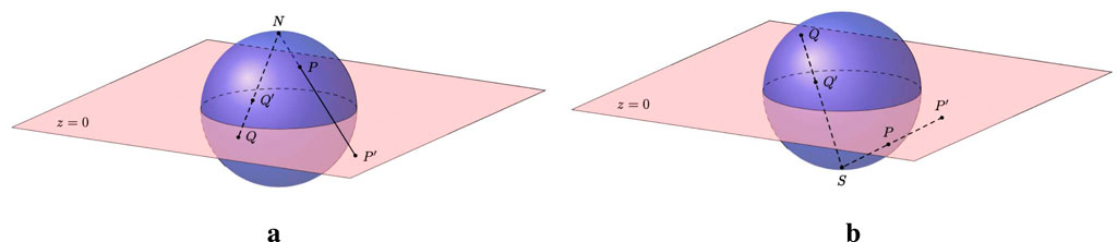
We first introduce stereographic projections of a unit vector $\widehat{\underline{\mathit{v}}}\in {\mathrm{S}}^2$ , needed in some of the flux balances. A unit vector $\widehat{\underline{\mathit{v}}}$ can be represented by a point $\mathrm{P}$ or $\mathrm{Q}$ on the unit sphere; see Figure 2. There are two stereographic projections of $\widehat{\underline{\mathit{v}}}$ , i.e., the projection from the north pole and from the south pole. To compute the stereographic projection from the north pole $\mathrm{N}$ , we have to compute the intersection of the line through $\mathrm{N}$ and $\mathrm{P}$ , given by

$\underline{\mathit{r}}\left(\lambda \right)=\left(\begin{array}{c}\hfill 0\hfill \\ \hfill 0\hfill \\ \hfill 1\hfill \end{array}\right)+\lambda \left(\begin{array}{c}\hfill v_1\hfill \\ \hfill v_2\hfill \\ \hfill v_3-1\hfill \end{array}\right),$

with the equator plane $z=0$ . In this way, we obtain the stereographic projection $\mathit{z}={\mathbf{S}}_{\mathrm{N}}(\widehat{\underline{\mathit{v}}})$ given by

${\mathbf{S}}_{\mathrm{N}}\left(\widehat{\underline{\mathit{v}}}\right)=\frac{1}{1-v_3}\left(\begin{array}{c}\hfill v_1\hfill \\ \hfill v_2\hfill \end{array}\right),(\mathrm{20a})$

which is defined for $v_3\ne 1$ . The latter condition means that $\mathrm{P}$ and $\mathrm{N}$ should not coincide. Using the relations $|\widehat{\underline{\mathit{v}}}{|}^2=1$ and $v_3\ne 1$ , we can compute the inverse $\widehat{\underline{\mathit{v}}}={\mathbf{S}}_{\mathrm{N}}^{-1}(\mathit{z})$ and find

${\mathbf{S}}_{\mathrm{N}}^{-1}\left(\mathit{z}\right)=\frac{1}{1+|\mathit{z}{|}^2}\left(\begin{array}{c}\hfill 2z_1\hfill \\ \hfill 2z_2\hfill \\ \hfill -1+|\mathit{z}{|}^2\hfill \end{array}\right).(\mathrm{20b})$

In a similar manner, we can determine the stereographic projection from the south pole and its inverse. These are given by

$\mathit{z}={\mathbf{S}}_{\mathrm{S}}\left(\widehat{\underline{\mathit{v}}}\right)=\frac{1}{1+v_3}\left(\begin{array}{c}\hfill v_1\hfill \\ \hfill v_2\hfill \end{array}\right),\widehat{\underline{\mathit{v}}}={\mathbf{S}}_{\mathrm{S}}^{-1}\left(\mathit{z}\right)=\frac{1}{1+|\mathit{z}{|}^2}\left(\begin{array}{c}\hfill 2z_1\hfill \\ \hfill 2z_2\hfill \\ \hfill 1-|\mathit{z}{|}^2\hfill \end{array}\right)(21)$

and are defined for $v_3\ne -1$ . Both projections are parameterizations of ${\mathrm{S}}^2$ , and in either case, an area element $\mathrm{d}S(\mathit{z})$ on $S^2$ generated by $\widehat{\underline{\mathit{v}}}$ is given by

$\mathrm{d}S\left(\mathit{z}\right)=\left|\frac{\partial \widehat{\underline{\mathit{v}}}}{\partial z_1}\times \frac{\partial \widehat{\underline{\mathit{v}}}}{\partial z_2}\right|\mathrm{d}\mathit{z}=\frac{4}{{\left(1+|\mathit{z}{|}^2\right)}^2}\mathrm{d}\mathit{z}≕J\left(\widehat{\underline{\mathit{v}}}\left(\mathit{z}\right)\right)\mathrm{d}\mathit{z}.(22)$

The choice for the stereographic projection depends on the direction of $\widehat{\underline{\mathit{v}}}$ . If $v_3>0$ , a suitable choice is the projection from the south pole; since then, the domain for $\mathit{z}$ is included in the interior of the disc $|\mathit{z}|\le 1$ . The projection from the north pole gives a domain outside this disc; see Figure 2. Likewise, if $v_3<0$ , the projection from the north pole is the proper choice.

Figure 2

Figure 2. Stereographic projections of the unit sphere ${\mathrm{S}}^2$ . (A) From the north pole N. (B) From the south pole S.

Assuming there is no energy lost, the most generic form of the luminous flux balance reads

${\int }_{\mathcal{A}}f\left(\mathit{x}\right)\mathrm{d}S\left(\mathit{x}\right)={\int }_{\mathit{m}\left(\mathcal{A}\right)}g\left(\mathit{y}\right)\mathrm{d}S\left(\mathit{y}\right),(23)$

for every subset $\mathcal{A}\subset \mathcal{X}$ and image set $\mathit{m}(\mathcal{A})\subset \mathcal{Y}$ , where $f(\mathit{x})$ and $g(\mathit{y})$ are the flux densities, to be specified shortly, at the source and target, respectively. Here, $\mathrm{d}S(\mathit{x})$ denotes an area element on the (curved) surface $\mathcal{S}$ describing the source and parameterized by $\mathit{x}$ . Analogously, $\mathrm{d}S(\mathit{y})$ is an area element on the target surface $\mathcal{T}$ , parameterized by $\mathit{y}$ . Equation 23 should hold for any subsets $\mathcal{A}\subset \mathcal{X}$ and $\mathit{m}(\mathcal{A})\subset \mathcal{Y}$ , so also for $\mathcal{A}=\mathcal{X}$ and $\mathit{m}(\mathcal{A})=\mathcal{Y}$ , giving the global luminous flux balance. This implies that an inverse design problem can only have a solution if $f$ and $g$ satisfy this global flux balance.

The precise form of the flux balance depends on the source and target. For the source, we consider two options: first, a planar source located in $z=0$ and emitting a parallel beam of light with $\widehat{\underline{\mathit{s}}}={\widehat{\underline{\mathit{e}}}}_z$ , and second, a point source located in the origin and emitting a conical beam of light with $\widehat{\underline{\mathit{s}}}={\widehat{\underline{\mathit{e}}}}_r$ . Both are zero-étendue (English: zero-extent) sources, meaning that the emitted beam has either a spatial or angular extent, but in the embedding four-dimensional phase space, it has zero volume; see Chaves [25]. For the planar source $\mathcal{S}=\{\underline{\mathit{r}}(\mathit{x})=(\mathit{x},0)|\mathit{x}\in \mathcal{X}\subset {\mathbb{R}}^2\}$ , $\mathit{x}={\mathit{q}}_{\mathrm{s}}$ are spatial coordinates (Cartesian/polar), $\mathrm{d}S(\mathit{x})=\mathrm{d}\mathit{x}$ , the area element in the source plane, and $f(\mathit{x})=M(\underline{\mathit{r}}(\mathit{x}))$ , the emittance, i.e., the luminous flux per unit area emitted by the source. The point source has no spatial extent but emits light rays in an angular domain, specified by $\widehat{\underline{\mathit{s}}}\in \mathcal{S}\subset {\mathrm{S}}^2$ . As parameterization, we choose a stereographic projection, either from the north or south pole, the area element $\mathrm{d}S(\mathit{x})=J(\widehat{\underline{\mathit{s}}}(\mathit{x}))\mathrm{d}\mathit{x}$ , cf. Equation 22, and $f(\mathit{x})=I_{\mathrm{s}}(\widehat{\underline{\mathit{s}}}(\mathit{x}))$ , the intensity of the source, i.e., the emitted luminous flux per unit solid angle. We can express both flux densities in the form $f=\tilde{f}◦{\mathbf{P}}_{\mathrm{s}}^{-1}$ , where $\tilde{f}=M$ and ${\mathbf{P}}_{\mathrm{s}}:(\mathit{x},0)\mapsto \mathit{x}$ , the trivial projection from $\mathcal{S}$ to $\mathcal{X}$ , for the planar source and $\tilde{f}=I_{\mathrm{s}}$ and ${\mathbf{P}}_{\mathrm{s}}={\mathbf{S}}_{\mathrm{N}}$ or ${\mathbf{P}}_{\mathrm{s}}={\mathbf{S}}_{\mathrm{S}}$ for the point source.

For the target, we consider the following cases; first, a near-field target located on a curved surface $\mathcal{T}=\{\underline{\mathit{r}}(\mathit{y})=(\mathit{y},v(\mathit{y}))|\mathit{y}\in \mathcal{Y}\subset {\mathbb{R}}^2\}$ , and second, a far-field target. For the near-field target, $\mathit{y}={\mathit{q}}_{\mathrm{t}}$ are spatial coordinates in a reference plane $z=z_{\mathrm{t}}$ , the area element

$\mathrm{d}S\left(\mathit{y}\right)=\left|\frac{\partial \underline{\mathit{r}}}{\partial y_1}\times \frac{\partial \underline{\mathit{r}}}{\partial y_2}\right|\mathrm{d}\mathit{y}=\sqrt{|\nabla v\left(\mathit{y}\right){|}^2+1}\mathrm{d}\mathit{y},$

and $g(\mathit{y})=E(\underline{\mathit{r}}(\mathit{y}))$ , the illuminance, i.e., the luminous flux per unit area incident on the target surface. The domain of a far-field target is an angular domain, determined by the transmitted rays with $\widehat{\underline{\mathit{t}}}\in \mathcal{T}\subset {\mathrm{S}}^2$ . Therefore, we choose for $\mathit{y}$ one of the two stereographic projections, for which $\mathrm{d}S(\mathit{y})=J(\widehat{\underline{\mathit{t}}}(\mathit{y}))\mathrm{d}\mathit{y}$ ; cf. Equation 22. However, $g(\mathit{y})=I_{\mathrm{t}}(\widehat{\underline{\mathit{r}}}(\mathit{y}))$ , the intensity in the target domain as a function of $\widehat{\underline{\mathit{r}}}$ , the unit direction vector directed straight from source to target domain, skipping all optical surfaces, rather than a function of $\widehat{\underline{\mathit{t}}}$ . In the far-field approximation, the distance from the source to target is large compared to the size of the optical system, specifically $|\underline{\mathit{r}}-d\widehat{\underline{\mathit{t}}}|/|\underline{\mathit{r}}|\ll 1$ , where $d$ is the distance from the optical surface to target, measured along a reflected ray; see, e.g., [4], pp. 59–60. The optical system is considered a point contracted at the origin, so we simply consider $g(\mathit{y})=I_{\mathrm{t}}(\widehat{\underline{\mathit{t}}}(\mathit{y}))$ . In addition, for the target, both flux densities can be unified in the expression $g=\tilde{g}◦{\mathbf{P}}_{\mathrm{t}}^{-1}$ , where for the near field $\tilde{g}=E$ and ${\mathbf{P}}_{\mathrm{t}}:(\mathit{y},v(\mathit{y}))\mapsto \mathit{y}$ is the orthogonal projection from $\mathcal{T}$ to $\mathcal{Y}$ , and where for the far-field target, $\tilde{g}=I_{\mathrm{t}}$ and either ${\mathbf{P}}_{\mathrm{t}}={\mathbf{S}}_{\mathrm{N}}$ or ${\mathbf{P}}_{\mathrm{t}}={\mathbf{S}}_{\mathrm{S}}$ .

5 Reflector and lens equations: a hierarchy of mathematical models

We present a hierarchy of mathematical models for optical systems with a zero-étendue source, based on three example systems, i.e., a parallel-to-far-field reflector, point-to-far-field lens, and parallel-to-near-field reflector. These example systems are selected based on the mathematical model (quadratic cost function, non-quadratic cost function, and generating function) but are otherwise arbitrary. Other choices like a parallel-to-far-field-lens (quadratic cost function) or point-to-near-field reflector (generating function) would be equally appropriate. In this section, we combine the geometrical equations with the conservation law for luminous flux.

5.1 Parallel-to-far-field reflector

We consider a light source located in the plane $z=0$ emitting a parallel beam of light, for which $\widehat{\underline{\mathit{s}}}={\widehat{\underline{\mathit{e}}}}_z$ . Light rays strike the reflector $\mathcal{R}$ defined by $z=u(\mathit{x})$ , $\mathit{x}\in \mathcal{X}\subset {\mathbb{R}}^2$ , and are reflected off in the direction $\widehat{\underline{\mathit{t}}}\in \mathcal{T}\subset {\mathrm{S}}^2$ . The reflected rays intersect an auxiliary plane $z=L$ , which we introduce to be able to determine an optical distance; see Figure 3. More precisely, to derive a geometrical equation for the reflector surface, we determine from Equation 10 the mixed characteristic of the first kind $W({\mathit{q}}_{\mathrm{s}},{\mathit{p}}_{\mathrm{t}})$ for an arbitrary ray with ${\mathit{q}}_{\mathrm{s}}=\mathit{x}$ and ${\mathit{p}}_{\mathrm{t}}={(t_1{t}_2)}^{\text{T}}$ , connecting the source with the plane $z=L$ . The point characteristic $V({\mathit{q}}_{\mathrm{s}},{\mathit{q}}_{\mathrm{t}})$ involved is given by

$V\left({\mathit{q}}_{\mathrm{s}},{\mathit{q}}_{\mathrm{t}}\right)=\left[{\mathrm{Q}}_{\mathrm{s}},{\mathrm{Q}}_{\mathrm{t}}\right]=u\left(\mathit{x}\right)+d,d=\sqrt{|{\mathit{q}}_{\mathrm{t}}-\mathit{x}{|}^2+{\left(L-u\left(\mathit{x}\right)\right)}^2},(24)$

where $d=d(\mathrm{P},{\mathrm{Q}}_{\mathrm{t}})$ is the distance between the points $\mathrm{P}(\mathit{x},u(\mathit{x}))$ and ${\mathrm{Q}}_{\mathrm{t}}({\mathit{q}}_{\mathrm{t}},L)$ , which are the points where the reflected ray hits the reflector and target plane, respectively, loosely referred to as intersection points. For the direction vector $\widehat{\underline{\mathit{t}}}$ of the reflected ray, we have

${\mathit{p}}_{\mathrm{t}}=\left(\begin{array}{c}\hfill t_1\hfill \\ \hfill t_2\hfill \end{array}\right)=\frac{1}{d}\left({\mathit{q}}_{\mathrm{t}}-\mathit{x}\right),t_3=\frac{1}{d}\left(L-u\left(\mathit{x}\right)\right).(25)$

Moreover, $\partial W/\partial {\mathit{q}}_{\mathrm{s}}=-{\mathit{p}}_{\mathrm{s}}=\mathbf{0}$ since $\widehat{\underline{\mathit{s}}}$ is perpendicular to the source plane, implying that $W=W({\mathit{p}}_{\mathrm{t}})$ . Elaborating the expression for $W$ , using the relations in Equations 24, 25, we find

$\begin{array}{cc}\hfill W\left({\mathit{p}}_{\mathrm{t}}\right)& =u\left(\mathit{x}\right)+d-{\mathit{q}}_{\mathrm{t}}\cdot {\mathit{p}}_{\mathrm{t}}\hfill \\ \hfill & =u\left(\mathit{x}\right)+\frac{1}{d}\left(|{\mathit{q}}_{\mathrm{t}}-\mathit{x}{|}^2+{\left(L-u\left(\mathit{x}\right)\right)}^2-{\mathit{q}}_{\mathrm{t}}\cdot \left({\mathit{q}}_{\mathrm{t}}-\mathit{x}\right)\right)\hfill \\ \hfill & =u\left(\mathit{x}\right)+\frac{1}{d}\left(-\mathit{x}\cdot \left({\mathit{q}}_{\mathrm{t}}-\mathit{x}\right)+d{t}_3\left(L-u\left(\mathit{x}\right)\right)\right)\hfill \\ \hfill & =u\left(\mathit{x}\right)\left(1-t_3\right)-\mathit{x}\cdot {\mathit{p}}_{\mathrm{t}}+L{t}_3.\hfill \end{array}$

Figure 3

Figure 3. Sketch of a parallel-to-far-field reflector.

To separate the variables $\mathit{x}$ (source) and ${\mathit{p}}_{\mathrm{t}}$ (target), we bring all terms that solely depend on $\widehat{\underline{\mathit{t}}}$ to the left-hand side, and we obtain

$\frac{W\left({\mathit{p}}_{\mathrm{t}}\right)-L{t}_3}{1-t_3}=u\left(\mathit{x}\right)-\frac{\mathit{x}\cdot {\mathit{p}}_{\mathrm{t}}}{1-t_3}.(26)$

Note that $t_3\ne 1$ since rays cannot pass straight through the reflector. Using the expressions for $d$ and $t_3$ , we can show that

$\frac{\partial W}{\partial L}=\frac{\partial d}{\partial L}-\frac{\partial {\mathit{q}}_{\mathrm{t}}}{\partial L}\cdot {\mathit{p}}_{\mathrm{t}},\frac{\partial d}{\partial L}={\mathit{p}}_{\mathrm{t}}\cdot \frac{\partial {\mathit{q}}_{\mathrm{t}}}{\partial L}+t_3,$

from which we readily conclude that the left-hand side in Equation 26 is independent of $L$ , which makes sense since a far-field target domain should not depend on the choice of a particular plane $z=L$ . As stated in Section 4, the proper choice to parameterize the target $\mathcal{T}$ is the stereographic projection from the north pole; thus, $\mathit{y}={\mathit{p}}_{\mathrm{t}}/(1-t_3)$ and $\mathcal{Y}={\mathbf{S}}_{\mathrm{N}}(\mathcal{T})$ ; cf. Equation 20. Substituting the expression for $\mathit{y}$ in Equation 26, we arrive at the geometrical equation

$u_1\left(\mathit{x}\right)+u_2\left(\mathit{y}\right)=c\left(\mathit{x},\mathit{y}\right),c\left(\mathit{x},\mathit{y}\right)=\mathit{x}\cdot \mathit{y},(27)$

where $u_1(\mathit{x})=u(\mathit{x})$ and $u_2(\mathit{y})=(L{t}_3-W({\mathit{p}}_{\mathrm{t}}))/(1-t_3)$ .

Referring to Section 3, a possible solution of Equation 27 is the max/max solution in Equation 13, which is a conjugate pair of Legendre–Fenchel transforms since $c(\mathit{x},\mathit{y})=\mathit{x}\cdot \mathit{y}$ . The necessary condition in Equation 14 and the matrix equation for the optical map in Equation 15 reduce to

$\mathit{y}-\nabla u_1\left(\mathit{x}\right)=\mathbf{0},(\mathrm{28a})$

$\mathrm{D}\mathit{m}=\mathit{P}\left(\mathit{x}\right),\mathit{P}\left(\mathit{x}\right)={\mathrm{D}}^2{u}_1\left(\mathit{x}\right).(\mathrm{28b})$

Recall that Equation 28b has to be supplemented with the transport boundary condition (Equation 16).

To close the model, we elaborate the flux balance in Equation 23. Substituting $f(\mathit{x})=M(\underline{\mathit{r}}(\mathit{x}))$ , $\mathrm{d}S(\mathit{x})=\mathrm{d}\mathit{x}$ , $g(\mathit{y})=I_{\mathrm{t}}(\widehat{\underline{\mathit{t}}}(\mathit{y}))$, and $\mathrm{d}S(\mathit{y})=J(\widehat{\underline{\mathit{t}}}(\mathit{y}))\mathrm{d}\mathit{y}$ , we obtain

${\int }_{\mathcal{A}}M\left(\underline{\mathit{r}}\left(\mathit{x}\right)\right)\mathrm{d}\mathit{x}={\int }_{\mathit{m}\left(\mathcal{A}\right)}{I}_{\mathrm{t}}\left(\widehat{\underline{\mathit{t}}}\left(\mathit{y}\right)\right)J\left(\widehat{\underline{\mathit{t}}}\left(\mathit{y}\right)\right)\mathrm{d}\mathit{y},$

for arbitrary $\mathcal{A}\subset \mathcal{X}$ and $\mathit{m}(\mathcal{A})\subset \mathcal{Y}$ . Substituting $\mathit{y}=\mathit{m}(\mathit{x})$ and the expression for $J(\widehat{\underline{\mathit{t}}}(\mathit{y}))$ , replacing $\widehat{\underline{\mathit{v}}}(\mathit{z})$ by $\widehat{\underline{\mathit{t}}}(\mathit{y})$ in Equation 22, we can rewrite the integral in the right-hand side and find

${\int }_{\mathcal{A}}M\left(\underline{\mathit{r}}\left(\mathit{x}\right)\right)\mathrm{d}\mathit{x}={\int }_{\mathcal{A}}{I}_{\mathrm{t}}\left(\widehat{\underline{\mathit{t}}}\left(\mathit{m}\left(\mathit{x}\right)\right)\right)\frac{4}{{\left(1+|\mathit{m}\left(\mathit{x}\right){|}^2\right)}^2}\det \left(\mathrm{D}\mathit{m}\right)\mathrm{d}\mathit{x},(29)$

where we used that $\det (\mathrm{D}\mathit{m})>0$ , which is correct because $\mathrm{D}\mathit{m}$ is either SPD or SND. Since Equation 29 should hold for arbitrary $\mathcal{A}\subset \mathcal{X}$ , we obtain the differential form

$\det \left(\mathrm{D}\mathit{m}\right)=\frac{1}{4}{\left(1+|\mathit{m}\left(\mathit{x}\right){|}^2\right)}^2\frac{M\left(\underline{\mathit{r}}\left(\mathit{x}\right)\right)}{I_{\mathrm{t}}\left(\widehat{\underline{\mathit{t}}}\left(\mathit{m}\left(\mathit{x}\right)\right)\right)}≕F\left(\mathit{x},\mathit{m}\left(\mathit{x}\right)\right),$

referred to as the Jacobian equation. Substituting $\mathit{m}=\nabla u_1$ , this equation reduces to the standard MA equation $\det ({\mathrm{D}}^2{u}_1)=F(\mathit{x},\nabla u_1(\mathit{x}))$ ; see, e.g., Gutiérrez [3].

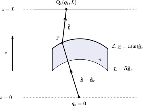
5.2 Point-to-far-field lens

We consider a point source located in the origin ${\mathrm{O}}_{\mathrm{s}}$ (position vector given by ${\mathit{q}}_{\mathrm{s}}=\mathit{0}$ and $z_{\mathrm{s}}=0$ ), emitting upward a conical beam of light with the direction vector $\widehat{\underline{\mathit{s}}}={\widehat{\underline{\mathit{e}}}}_r$ . Light rays hit a lens of refractive index $n$ ; see Figure 4. The first (entrance) surface is spherical with center ${\mathrm{O}}_{\mathrm{s}}$ and radius $R$ ; hence, rays are not refracted there; however, the second (exit) surface is freeform and given by the parameterization $\underline{\mathit{r}}(\widehat{\underline{\mathit{s}}})=u(\widehat{\underline{\mathit{s}}})\widehat{\underline{\mathit{s}}}$ . Rays are refracted at the exit surface and arrive at an auxiliary plane $z=L>0$ . To derive a geometrical equation for the freeform surface, we evaluate the angular characteristic $T({\mathit{p}}_{\mathrm{s}},{\mathit{p}}_{\mathrm{t}})$ defined in Equation 11 for an arbitrary ray connecting the source with the plane $z=L$ . The point characteristic $V({\mathit{q}}_{\mathrm{s}},{\mathit{q}}_{\mathrm{t}})$ needed to evaluate $T({\mathit{p}}_{\mathrm{s}},{\mathit{p}}_{\mathrm{t}})$ is given by

$\begin{array}{cc}\hfill V\left({\mathit{q}}_{\mathrm{s}},{\mathit{q}}_{\mathrm{t}}\right)& =\left[{\mathrm{O}}_{\mathrm{s}},{\mathrm{Q}}_{\mathrm{t}}\right]=R+n\left(u\left(\widehat{\underline{\mathit{s}}}\right)-R\right)+d\hfill \\ \hfill & d=\sqrt{|{\mathit{q}}_{\mathrm{t}}-u\left(\widehat{\underline{\mathit{s}}}\right){\mathit{p}}_{\mathrm{s}}{|}^2+{\left(L-u\left(\widehat{\underline{\mathit{s}}}\right)s_3\right)}^2}\hfill \end{array}(30)$

where $d=d(\mathrm{P},{\mathrm{Q}}_{\mathrm{t}})$ is the distance between the points $\mathrm{P}(u(\widehat{\underline{\mathit{s}}}){\mathit{p}}_{\mathrm{s}},u(\widehat{\underline{\mathit{s}}})s_3)$ and ${\mathrm{Q}}_{\mathrm{t}}({\mathit{q}}_{\mathrm{t}},L)$ , which are the intersection points of the refracted ray with exit surface and target screen, respectively. The direction vector $\widehat{\underline{\mathit{t}}}$ of the refracted ray is given by

${\mathit{p}}_{\mathrm{t}}=\left(\begin{array}{c}\hfill t_1\hfill \\ \hfill t_2\hfill \end{array}\right)=\frac{1}{d}\left({\mathit{q}}_{\mathrm{t}}-u\left(\widehat{\underline{\mathit{s}}}\right){\mathit{p}}_{\mathrm{s}}\right),t_3=\frac{1}{d}\left(L-u\left(\widehat{\underline{\mathit{s}}}\right)s_3\right).(31)$

Note that $\partial T/\partial {\mathit{p}}_{\mathrm{s}}={\mathit{q}}_{\mathrm{s}}=\mathit{0}$ , implying that $T=T({\mathit{p}}_{\mathrm{t}})$ . Evaluating the expression for $T({\mathit{p}}_{\mathrm{t}})$ in Equation 11 using the relations in Equations 30, 31, we obtain

$\begin{array}{cc}\hfill T\left({\mathit{p}}_{\mathrm{t}}\right)& =R+n\left(u\left(\widehat{\underline{\mathit{s}}}\right)-R\right)+d-{\mathit{q}}_{\mathrm{t}}\cdot {\mathit{p}}_{\mathrm{t}}\hfill \\ \hfill & =\left(1-n\right)R+nu\left(\widehat{\underline{\mathit{s}}}\right)+\frac{1}{d}\left(|{\mathit{q}}_{\mathrm{t}}-u\left(\widehat{\underline{\mathit{s}}}\right){\mathit{p}}_{\mathrm{s}}{|}^2+{\left(L-u\left(\widehat{\underline{\mathit{s}}}\right)s_3\right)}^2\right.\hfill \\ \hfill & -\left.{\mathit{q}}_{\mathrm{t}},\cdot ,\left({\mathit{q}}_{\mathrm{t}}-u\left(\widehat{\underline{\mathit{s}}}\right){\mathit{p}}_{\mathrm{s}}\right)\right)\hfill \\ \hfill & =\left(1-n\right)R+nu\left(\widehat{\underline{\mathit{s}}}\right)+\frac{1}{d}\left(-u\left(\widehat{\underline{\mathit{s}}}\right){\mathit{p}}_{\mathrm{s}}\right)\cdot \left({\mathit{q}}_{\mathrm{t}}-u\left(\widehat{\underline{\mathit{s}}}\right){\mathit{p}}_{\mathrm{s}}\right)\hfill \\ \hfill & +\left.d,t_3,\left(L-u\left(\widehat{\underline{\mathit{s}}}\right)s_3\right)\right)\hfill \\ \hfill & =\left(1-n\right)R+nu\left(\widehat{\underline{\mathit{s}}}\right)-u\left(\widehat{\underline{\mathit{s}}}\right){\mathit{p}}_{\mathrm{s}}\cdot {\mathit{p}}_{\mathrm{t}}+t_3\left(L-u\left(\widehat{\underline{\mathit{s}}}\right)s_3\right)\hfill \\ \hfill & =\left(1-n\right)R+\left(n-\widehat{\underline{\mathit{s}}}\cdot \widehat{\underline{\mathit{t}}}\right)u\left(\widehat{\underline{\mathit{s}}}\right)+L{t}_3.\hfill \end{array}(32)$

To derive the last expression for $T$ in Equation 32, we substituted the relation $\widehat{\underline{\mathit{s}}}\cdot \widehat{\underline{\mathit{t}}}={\mathit{p}}_{\mathrm{s}}\cdot {\mathit{p}}_{\mathrm{t}}+s_3{t}_3$ . Next, we move all terms that solely depend on $\widehat{\underline{\mathit{t}}}$ and the constant $(1-n)R$ to the left-hand side and find

$T\left({\mathit{p}}_{\mathrm{t}}\right)-L{t}_3+\left(n-1\right)R=\left(n-\widehat{\underline{\mathit{s}}}\cdot \widehat{\underline{\mathit{t}}}\right)u\left(\widehat{\underline{\mathit{s}}}\right).(33)$

Differentiating the first expression in Equation 32 with respect to $L$ and combining the expression for $d$ with Equation 31, we obtain

$\frac{\partial T}{\partial L}=\frac{\partial d}{\partial L}-\frac{\partial {\mathit{q}}_{\mathrm{t}}}{\partial L}\cdot {\mathit{p}}_{\mathrm{t}},\frac{\partial d}{\partial L}={\mathit{p}}_{\mathrm{t}}\cdot \frac{\partial {\mathit{q}}_{\mathrm{t}}}{\partial L}+t_3,$

from which we readily see that the left-hand side in Equation 33 is independent of $L$ , as anticipated.

Figure 4

Figure 4. Sketch of a point-to-far-field lens.

To separate source and target coordinates, analogous to Equation 27, we have to take the logarithm of the left- and right-hand sides of Equation 33. Note that $n-\widehat{\underline{\mathit{s}}}\cdot \widehat{\underline{\mathit{t}}}>0$ and $u(\widehat{\underline{\mathit{s}}})>0$ ; consequently, the left-hand side is positive as well, and we can take the logarithms. In addition, we substitute the stereographic projections (from the south pole) $\mathit{x}$ of $\widehat{\underline{\mathit{s}}}$ and $\mathit{y}$ of $\widehat{\underline{\mathit{t}}}$ since both $\widehat{\underline{\mathit{s}}}$ and $\widehat{\underline{\mathit{t}}}$ are directed upward; cf. Equation 21. In this way, we obtain

$u_1\left(\mathit{x}\right)+u_2\left(\mathit{y}\right)=c\left(\mathit{x},\mathit{y}\right),(\mathrm{34a})$

where the variables $u_1(\mathit{x})$ and $u_2(\mathit{y})$ and the cost function $c(\mathit{x},\mathit{y})$ are defined by

$u_1\left(\mathit{x}\right)=\log u\left(\widehat{\underline{\mathit{s}}}\left(\mathit{x}\right)\right),(\mathrm{34b})$

$u_2\left(\mathit{y}\right)=-\log \left(T\left({\mathit{p}}_{\mathrm{t}}\left(\mathit{y}\right)\right)-L{t}_3\left(\mathit{y}\right)+\left(n-1\right)R\right),(\mathrm{34c})$

$c\left(\mathit{x},\mathit{y}\right)=-\log \left(n-\widehat{\underline{\mathit{s}}}\left(\mathit{x}\right)\cdot \widehat{\underline{\mathit{t}}}\left(\mathit{y}\right)\right).(\mathrm{34d})$

Formulated in terms of stereographic coordinates, the cost function reads

$c\left(\mathit{x},\mathit{y}\right)=-\log \left(n-1+\frac{2|\mathit{x}-\mathit{y}{|}^2}{\left(1+|\mathit{x}{|}^2\right)\left(1+|\mathit{y}{|}^2\right)}\right),$

which is no longer quadratic. A possible solution of Equation 34a is the $c$ -convex pair in Equation 13, for which the necessary condition (Equation 14) holds. For the optical map, matrix Equation 15 accompanied with the transport boundary condition (Equation 16) is given.

Referring to Section 4, in the far-field approximation, the luminous flux balance reads

${\int }_{\mathcal{A}}{I}_{\mathrm{s}}\left(\widehat{\underline{\mathit{s}}}\left(\mathit{x}\right)\right)J\left(\widehat{\underline{\mathit{s}}}\left(\mathit{x}\right)\right)\mathrm{d}\mathit{x}={\int }_{\mathit{m}\left(\mathcal{A}\right)}{I}_{\mathrm{t}}\left(\widehat{\underline{\mathit{t}}}\left(\mathit{y}\right)\right)J\left(\widehat{\underline{\mathit{t}}}\left(\mathit{y}\right)\right)\mathrm{d}\mathit{y},(35)$

for arbitrary $\mathcal{A}\subset \mathcal{X}$ and image set $\mathit{m}(\mathcal{A})\subset \mathcal{Y}$ . To derive the differential form, we substitute the expressions for $J(\widehat{\underline{\mathit{s}}}(\mathit{x}))$ and $J(\widehat{\underline{\mathit{t}}}(\mathit{y}))$ , according to Equation 22, and subsequently substitute $\mathit{y}=\mathit{m}(\mathit{x})$ . Assuming $\det (\mathrm{D}\mathit{m})>0$ , we obtain

$\det \left(\mathrm{D}\mathit{m}\right)={\left(\frac{1+|\mathit{m}\left(\mathit{x}\right){|}^2}{1+|\mathit{x}{|}^2}\right)}^2\frac{I_{\mathrm{s}}\left(\mathit{x}\right)}{I_{\mathrm{t}}\left(\mathit{m}\left(\mathit{x}\right)\right)}≕F\left(\mathit{x},\mathit{m}\left(\mathit{x}\right)\right).$

Combining this equation with the matrix equation in Equation 15, we obtain the GMA equation $\det ({\mathrm{D}}^2{u}_1-{\mathrm{D}}_{\mathit{x}\mathit{x}}c)=\det \left(C(\mathit{x},\mathit{m}(\mathit{x}))\right.F(\mathit{x},\mathit{m}(\mathit{x}))$ .

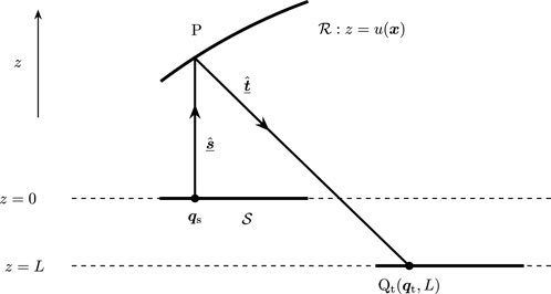
5.3 Parallel-to-near-field reflector

The last example concerns a planar source, located in $z=0$ , emitting a parallel beam of light rays in the direction $\widehat{\underline{\mathit{s}}}={\widehat{\underline{\mathit{e}}}}_z$ , consequently ${\mathit{p}}_{\mathrm{s}}=\mathbf{0}$ , which hits a reflector $\mathcal{R}$ given by $z=u(\mathit{x})$ , with $\mathit{x}={\mathit{q}}_{\mathrm{s}}$ spatial coordinates in the source domain, and are reflected off in the direction $\widehat{\underline{\mathit{t}}}$ and lands at a target surface given by $z=v(\mathit{y})$ , with $\mathit{y}={\mathit{q}}_{\mathrm{t}}$ spatial coordinates in the reference plane $z=z_{\mathrm{t}}=0$ . Thus, source and target planes coincide; see Figure 5. We evaluate Hamilton’s point characteristic and find

$\begin{array}{c}\hfill V\left({\mathit{q}}_{\mathrm{s}},{\mathit{q}}_{\mathrm{t}}\right)=\left[{\mathrm{Q}}_{\mathrm{s}},{\mathrm{Q}}_{\mathrm{t}}\right]\hfill \\ =u\left(\mathit{x}\right)+d,d=\sqrt{|\mathit{y}-\mathit{x}{|}^2+{\left(v\left(\mathit{y}\right)-u\left(\mathit{x}\right)\right)}^2},\hfill \end{array}$

where $d=d(\mathrm{P},{\mathrm{Q}}_{\mathrm{t}})$ is the distance between the intersection points $\mathrm{P}(\mathit{x},u(\mathit{x}))$ and ${\mathrm{Q}}_{\mathrm{t}}(\mathit{y},v(\mathit{y}))$ of the reflected ray with the reflector and the target surface, respectively. Since $\partial V/\partial {\mathit{q}}_{\mathrm{s}}=-{\mathit{p}}_{\mathrm{s}}=\mathbf{0}$ , we find that $V=V({\mathit{q}}_{\mathrm{t}})$ . In this case, it is no longer possible to separate the source and target coordinates $\mathit{x}$ and $\mathit{y}$ like in Equation 27 or (Equation 34a). Instead, we write

$u_2\left(\mathit{y}\right)=H\left(\mathit{x},\mathit{y},u_1\left(\mathit{x}\right)\right),H\left(\mathit{x},\mathit{y},w\right)=w+\sqrt{|\mathit{y}-\mathit{x}{|}^2+{\left(v\left(\mathit{y}\right)-w\right)}^2},(36)$

where $u_1(\mathit{x})=u(\mathit{x})$ and $u_2(\mathit{y})=V({\mathit{q}}_{\mathrm{t}})$ . Straightforward differentiation gives $H_w(\mathit{x},\mathit{y},\cdot )>0$ , implying that for fixed $\mathit{x},\mathit{y}$ , the inverse $G(\mathit{x},\mathit{y},\cdot )=H^{-1}(\mathit{x},\mathit{y},\cdot )$ exists. Therefore, we can explicitly determine $u_1(\mathit{x})$ from Equation 36, and we obtain

$u_1\left(\mathit{x}\right)=G\left(\mathit{x},\mathit{y},u_2\left(\mathit{y}\right)\right),G\left(\mathit{x},\mathit{y},w\right)=\frac{1}{2}\left(w+v\left(\mathit{y}\right)-\frac{|\mathit{y}-\mathit{x}{|}^2}{w-v\left(\mathit{y}\right)}\right).(37)$

A possible solution of Equations 36, 37 is the $G$ -convex $H$ -concave pair in Equation 17, for which the necessary condition (18) holds. The matrix equation for $\mathit{m}$ is given in Equation 15 with matrices $\mathit{C}$ and $\mathit{P}$ defined in Equation 19. Recall that these matrices explicitly depend on $u_1(\mathit{x})$ . Obviously, also the transport boundary condition (16) holds.

Figure 5

Figure 5. Sketch of a parallel-to-near-field reflector.

Making the proper choices for the flux densities and area elements, the flux balance (23) reduces to

${\int }_{\mathcal{A}}M\left(\underline{\mathit{r}}\left(\mathit{x}\right)\right)\mathrm{d}\mathit{x}={\int }_{\mathit{m}\left(\mathcal{A}\right)}E\left(\underline{\mathit{r}}\left(\mathit{y}\right)\right)\sqrt{|\nabla v\left(\mathit{y}\right){|}^2+1}\mathrm{d}\mathit{y},(38)$

for an arbitrary set $\mathcal{A}\subset \mathcal{X}$ and image set $\mathit{m}(\mathcal{A})\subset \mathcal{Y}$ , where $M(\underline{\mathit{r}}(\mathit{x}))$ and $E(\underline{\mathit{r}}(\mathit{y}))$ denote the emittance and illuminance of the source and target, respectively. Substituting $\mathit{y}=\mathit{m}(\mathit{x})$ , assuming $\det (\mathrm{D}\mathit{m})>0$ , we obtain

$\det \left(\mathrm{D}\mathit{m}\right)=\frac{1}{\sqrt{|\nabla v\left(\mathit{m}\left(\mathit{x}\right)\right){|}^2+1}}\frac{M\left(\underline{\mathit{r}}\left(\mathit{x}\right)\right)}{E\left(\underline{\mathit{r}}\left(\mathit{m}\left(\mathit{x}\right)\right)\right)}≕F\left(\mathit{x},\mathit{m}\left(\mathit{x}\right)\right).$

Combining this equation with Equation 15 and the matrices $\mathit{C}$ and $\mathit{P}$ defined in Equation 19, we obtain the equation $\det ({\mathrm{D}}_{\mathit{x}\mathit{x}}\tilde{H})=\det \left(\mathit{C}(\mathit{x},\mathit{m}(\mathit{x}),u_1(\mathit{x}))\right.F(\mathit{x},\mathit{m}(\mathit{x}))$ , referred to as the GJ equation.

5.4 Summary of mathematical models

All mathematical models considered consist of a geometrical equation, a (zero-gradient) condition for a stationary point, a matrix equation for the optical map coupled to the transport boundary condition, and a luminous flux balance $\det (\mathrm{D}\mathit{m})=F(\mathit{x},\mathit{m}(\mathit{x}))$ . The conditions for the stationary point read

$\text{cost\hspace{0.17em}function}{\nabla }_{\mathit{x}}c\left(\mathit{x},\mathit{y}\right)-\nabla u_1\left(\mathit{x}\right)=\mathbf{0},(\mathrm{39a})$

$\text{generating\hspace{0.17em}\hspace{0.17em}function}{\nabla }_{\mathit{x}}\tilde{H}\left(\mathit{x},\mathit{y}\right)=\mathbf{0}.(\mathrm{39b})$

Substituting the optical map $\mathit{y}=\mathit{m}(\mathit{x})$ and differentiating with respect to $\mathit{x}$ gives the matrix equation $\mathit{C}\mathrm{D}\mathit{m}=\mathit{P}$ , where the matrices $\mathit{C}$ and $\mathit{P}$ are given by

$\text{quadratic\hspace{0.17em}\hspace{0.17em}cost\hspace{0.17em}\hspace{0.17em}function}\mathit{C}=\mathit{I},\mathit{P}={\mathrm{D}}^2{u}_1,(\mathrm{40a})$

$\text{general\hspace{0.17em}\hspace{0.17em}cost\hspace{0.17em}\hspace{0.17em}function}\mathit{C}={\mathrm{D}}_{\mathit{x}\mathit{y}}c,\mathit{P}={\mathrm{D}}^2{u}_1-{\mathrm{D}}_{\mathit{x}\mathit{x}}c,(\mathrm{40b})$

$\text{generating\hspace{0.17em}\hspace{0.17em}function}\mathit{C}={\mathrm{D}}_{\mathit{x}\mathit{y}}\tilde{H},\mathit{P}=-{\mathrm{D}}_{\mathit{x}\mathit{x}}\tilde{H}.(\mathrm{40c})$

Combining the matrix equation for $\mathit{m}$ with the flux balance gives

$\det \left(\mathit{C}\right)F\left(\mathit{x},\mathit{m}\left(\mathit{x}\right)\right)=\det \left(\mathit{P}\right),$

which we refer to as the luminous flux constraint. Note that for the cost-function model, the matrices $\mathit{C}$ and $\mathit{P}$ explicitly depend on $\mathit{x}$ and $\mathit{m}(\mathit{x})$ ; on the other hand, for the generating-function model, both matrices in addition depend on $u_1(\mathit{x})$ . In [26], we have given a similar overview of mathematical models of 16 base optical systems.

In the next section, we outline numerical methods to compute the optical map $\mathit{y}=\mathit{m}(\mathit{x})$ and the auxiliary variable $u_1(\mathit{x})$ . The shape/location of the optical surface is then reconstructed from a simple algebraic equation, i.e., $u(\mathit{x})=u_1(\mathit{x})$ for the parallel-to-far-field and parallel-to-near-field reflectors and $u(\widehat{\underline{\mathit{s}}}(\mathit{x}))={\mathrm{e}}^{u_1(\mathit{x})}$ for the parallel-to-far-field lens.

6 Iterative least-squares methods

In this section, we outline iterative least-squares methods for the models presented in the previous section, starting with the base scheme for the cost-function models and adding modifications for the generation-function model. A detailed account of these methods is presented in a series of theses—see [27]; [23]; [4]—and papers—see [13]; [28]; [14, 29]; [15–18]; [26].

Base scheme for cost function

To compute the layout of the optical system, we apply a two-stage method, i.e., we first compute the optical map $\mathit{m}$ and subsequently, the auxiliary variable $u_1$ and possibly $u_2$ , from which we trivially can compute the shape/location of the optical surface(s). We employ a uniform rectangular grid covering the parameter space of the source domain.

We iteratively compute a symmetric matrix $\mathit{P}$ as approximation of the symmetric part of $\mathit{C}\mathrm{D}\mathit{m}$ , satisfying $\det (\mathit{P})=\det (\mathit{C}(\cdot ,\mathit{m}))F(\cdot ,\mathit{m})$ , and a vector field $\mathit{b}:\partial \mathcal{X}\to \partial \mathcal{Y}$ , from which we subsequently compute $\mathit{m}$ . Our solution strategy is then to minimize the functionals

$\begin{array}{ll}\hfill & \hfill J_{\mathrm{I}}\left[\mathit{m},\mathit{P}\right]=\frac{1}{2}{\int }_{\mathcal{X}}||\mathit{C}\mathrm{D}\mathit{m}-\mathit{P}|{|}_{\mathrm{F}}^2\mathrm{d}\mathit{x},\\ \hfill & \hfill \text{subject t\hspace{0.17em}o}\det \left(\mathit{P}\right)=\det \left(\mathit{C}\left(\cdot ,\mathit{m}\right)\right)F\left(\cdot ,\mathit{m}\right),\end{array}(\mathrm{41a})$

$J_{\mathrm{B}}\left[\mathit{m},\mathit{b}\right]=\frac{1}{2}{\oint }_{\partial \mathcal{X}}|\mathit{m}-\mathit{b}{|}_2^2\mathrm{d}s,(\mathrm{41b})$

$J\left[\mathit{m},\mathit{P},\mathit{b}\right]=\alpha J_{\mathrm{I}}\left[\mathit{m},\mathit{P}\right]+\left(1-\alpha \right)J_{\mathrm{B}}\left[\mathit{m},\mathit{b}\right],\left(0<\alpha <1\right),(\mathrm{41c})$

where $||\cdot |{|}_{\mathrm{F}}$ denotes the Frobenius norm. The minimization of $J_{\mathrm{B}}[\mathit{m},\mathit{b}]$ is to enforce the transport boundary condition (16). Given an initial guess ${\mathit{m}}^0$ , the iteration scheme then reads

${\mathit{P}}^{k+1}={\mathrm{argmin}}_{\mathit{P}\in \mathcal{P}\left({\mathit{m}}^k\right)}{J}_{\mathrm{I}}\left[{\mathit{m}}^k,\mathit{P}\right],(\mathrm{42a})$

${\mathit{b}}^{k+1}={\mathrm{argmin}}_{\mathit{b}\in \mathcal{B}}{J}_{\mathrm{B}}\left[{\mathit{m}}^k,\mathit{b}\right],(\mathrm{42b})$

${\mathit{m}}^{k+1}={\mathrm{argmin}}_{\mathit{m}\in \mathcal{M}}J\left[\mathit{m},{\mathit{P}}^{k+1},{\mathit{b}}^{k+1}\right],(\mathrm{42c})$

where the corresponding function spaces are given by

$\mathcal{P}\left(\mathit{m}\right)=\left\{\mathit{P}n\in o{C}^{1}ne{\left(\mathcal{X}\right)}^{2\times 2}e|e{\mathit{P}}^{\mathrm{T}}e=e\mathit{P}e,e\det \left(\mathit{P}\right)e=e\det \left(\mathit{C}\left(\cdot ,\mathit{m}\left(\cdot \right)\right)\right)eF\left(\cdot ,\mathit{m}\left(\cdot \right)\right)\right\},(\mathrm{43a})$

$\mathcal{B}=\left\{\mathit{b}\in C{\left(\partial \mathcal{X}\right)}^2|\mathit{b}\left(\mathit{x}\right)\in \partial \mathcal{Y}\right\},(\mathrm{43b})$

$\mathcal{M}=C^2{\left(\mathcal{X}\right)}^2.(\mathrm{43c})$

In common parlance, $\mathcal{P}(\mathit{m})$ is the space of $2\times 2$ matrix functions that are continuously differentiable on $\mathcal{X}$ , are symmetric, and satisfy the luminous flux constraint. $\mathcal{B}$ is the space of continuous vector functions that map the boundary $\partial \mathcal{X}$ to the boundary $\partial \mathcal{Y}$ .

The minimization of $J_{\mathrm{I}}[\mathit{m},\mathit{P}]$ to compute $\mathit{P}$ can be performed point-wise and requires the solution of a constrained minimization problem. $\mathit{P}$ has to be either SPD or SND, which can be enforced by a constraint on $\mathrm{t}\mathrm{r}(\mathit{P})$ . The minimization of $J_{\mathrm{B}}[\mathit{m},\mathit{b}]$ to compute $\mathit{b}$ is a piecewise projection of $\mathit{m}$ on $\partial \mathcal{X}$ . For the minimization of $J[\mathit{m},\mathit{P},\mathit{b}]$ , we impose the first variation with respect to $\mathit{m}$ to vanish, i.e.,

$\delta J\left[\mathit{m},\mathit{P},\mathit{b}\right]\left(\mathit{\eta }\right)=\underset{\epsilon \to 0}{\lim }\frac{1}{\epsilon }\left(J\left[\mathit{m}+\epsilon \mathit{\eta },\mathit{P},\mathit{b}\right]-J\left[\mathit{m},\mathit{P},\mathit{b}\right]\right)=0,(44)$

for arbitrary $\mathit{\eta }\in C^2{(\mathcal{X})}^2$ . Evaluating this limit, applying Gauss’s theorem and the fundamental lemma of calculus of variations ([30], p. 185), we derive the following coupled boundary value problem (BVP) for $\mathit{m}$:

$\nabla \cdot \left({\mathit{C}}^{\mathrm{T}}\mathit{C}\mathrm{D}\mathit{m}\right)=\nabla \cdot \left({\mathit{C}}^{\mathrm{T}}\mathit{P}\right),\mathit{x}\in \mathcal{X},(\mathrm{45a})$

$\left(1-\alpha \right)\mathit{m}+\alpha \left({\mathit{C}}^{\mathrm{T}}\mathit{C}\mathrm{D}\mathit{m}\right)\widehat{\mathit{n}}=\left(1-\alpha \right)\mathit{b}+\alpha {\mathit{C}}^{\mathrm{T}}\mathit{P}\widehat{\mathit{n}},\mathit{x}\in \partial \mathcal{X},(\mathrm{45b})$

where $\widehat{\mathit{n}}$ is the unit outward normal on $\partial \mathcal{X}$ . The divergence of a $2\times 2$ matrix function $\mathit{A}=({\mathit{a}}_1{\mathit{a}}_2)$ is defined as $\nabla \cdot \mathit{A}=\left(\begin{array}{c}\hfill \nabla \cdot {\mathit{a}}_1\hfill \\ \hfill \nabla \cdot {\mathit{a}}_2\hfill \end{array}\right)$ . For discretization of the BVP in (Equation 45), we employ the standard finite volume method ([4], pp. Appendix B).

Next, upon convergence of the iteration (42), we compute $u_1$ from (Equation 39a) by minimizing the functional

$I\left[u_1\right]=\frac{1}{2}{\int }_{\mathcal{X}}|{\nabla }_{\mathit{x}}c\left(\cdot ,\mathit{m}\right)-\nabla u_1{|}_2^2\mathrm{d}\mathit{x}.$

Analogous to the derivation of (Equation 45), we set the first variation $\delta I[u_1](v)=0$ for arbitrary $v\in C^2(\mathcal{X})$ , to obtain the Neumann problem

${\nabla }^2{u}_1=\nabla \cdot {\nabla }_{\mathit{x}}c\left(\cdot ,\mathit{m}\right),\mathit{x}\in \mathcal{X},(\mathrm{46a})$

$\nabla u_1\cdot \widehat{\mathit{n}}={\nabla }_{\mathit{x}}c\left(\cdot ,\mathit{m}\right)\cdot \widehat{\mathit{n}},\mathit{x}\in \partial \mathcal{X}.(\mathrm{46b})$

We employ standard finite differences for the BVP in 46. $u_1$ is determined up to an additive constant, which translates in an additive constant in the location of the parallel-to-far-field reflector and a multiplicative constant for the location of the point-to-far-field lens. To compute a unique solution from 46 we either fix the distance from the source to optical surface along a specific ray, or prescribe an average for $u_1$ .

Extension to generating function

The optical map $\mathit{m}$ and the variable $u_1$ have to be computed simultaneously since the matrices $\mathit{C}$ and $\mathit{P}$ depend on both variables. Like in the previous case, the optical map satisfies the equation $\mathit{C}\mathrm{D}\mathit{m}=\mathit{P}$ , with the matrices $\mathit{C}$ and $\mathit{P}$ defined in Equation 40c, and the luminous flux balance $\det (\mathrm{D}\mathit{m})=F$ . Consequently, the functional $J_{\mathrm{I}}[\mathit{m},\mathit{P}]$ remains the same, albeit with different matrices $\mathit{C}$ and $\mathit{P}$ . The variable $u_1$ has to be computed from Equation 39b, for which we introduce the functional

$\begin{array}{cc}\hfill I\left[u_1,\mathit{m}\right]& =\frac{1}{2}{\int }_{\mathcal{X}}{\left|{\nabla }_{\mathit{x}}\tilde{H}\left(\cdot ,\mathit{m}\right)\right|}_2^2\mathrm{d}\mathit{x}\hfill \\ \hfill & =\frac{1}{2}{\int }_{\mathcal{X}}{\left|{\nabla }_{\mathit{x}}H\left(\cdot ,\mathit{m},u_1\right)+H_w\left(\cdot ,\mathit{m},u_1\right)\nabla u_1\right|}_2^2\mathrm{d}\mathit{x}.\hfill \end{array}(47)$

To minimize the functional in Equation 47, we require $\delta I[u_1,\mathit{m}](v)=0$ for arbitrary $v\in C^2(\mathcal{X})$ , with $\delta I[u_1,\mathit{m}](v)$ the first variation in $I$ with respect to $u_1$ , defined analogously to Equation 44. This way we can derive the BVP

$\nabla \cdot \left(H_w{\nabla }_{\mathit{x}}H+H_w^2\nabla u_1\right)=\frac{1}{2}\frac{\mathrm{d}}{\mathrm{d}w}{\left|{\nabla }_{\mathit{x}}H+H_w\nabla u_1\right|}_2^2,\mathit{x}\in \mathcal{X},(\mathrm{48a})$

$H_w\left({\nabla }_{\mathit{x}}H+H_w\nabla u_1\right)\cdot \widehat{\mathit{n}}=0,\mathit{x}\in \partial \mathcal{X}.(\mathrm{48b})$

We employ the standard finite volume method for discretization. We can show that also the solution of the BVP in Equation 48 is determined up to an additive constant and compute a unique solution prescribing the average value of $u_1$ ; see ([4], pp. 166–167) for more details. Finally, given an initial guess ${\mathit{m}}^0$ and $u_1^0$ , the iteration scheme then reads

${\mathit{P}}^{k+1}={\mathrm{argmin}}_{\mathit{P}\in \mathcal{P}\left({\mathit{m}}^k\right)}{J}_{\mathrm{I}}\left[{\mathit{m}}^k,u_1^k,\mathit{P}\right],(\mathrm{49a})$

${\mathit{b}}^{k+1}={\mathrm{argmin}}_{\mathit{b}\in \mathcal{B}}{J}_{\mathrm{B}}\left[{\mathit{m}}^k,\mathit{b}\right],(\mathrm{49b})$

${\mathit{m}}^{k+1}={\mathrm{argmin}}_{\mathit{m}\in \mathcal{M}}J\left[\mathit{m},u_1^k,{\mathit{P}}^{k+1},{\mathit{b}}^{k+1}\right],(\mathrm{49c})$

$u_1^{k+1}={\mathrm{argmin}}_{v\in \mathcal{U}}I\left[v,{\mathit{m}}^{k+1}\right],(\mathrm{49d})$

with $\mathcal{U}=C^2(\mathcal{X})$ , where we have included $u_1^k$ in the argument list of $J_{\mathrm{I}}$ and $J$ to denote their implicit dependence on $u_1$ via the matrix $\mathit{C}$ .

7 Numerical examples

We present two numerical examples, viz. the point-to-far-field lens discussed in Section 5.2 and the parallel-to-near-field reflector from Section 5.3.

7.1 Point-to-far-field lens

We consider a point source, located in the origin ${\mathrm{O}}_{\mathrm{s}}$ of the source plane $z=0$ , emitting upward a beam of light with uniform intensity $I_{\mathrm{s}}(\widehat{\underline{\mathit{s}}}(\mathit{x}))$ on the circular stereographic source domain $\mathcal{X}=\{\mathit{x}\in {\mathbb{R}}^2||\mathit{x}|<0.2\}$ . In terms of spherical coordinates $(\varphi ,\theta )$ , this corresponds to the domain $0\le \varphi \le \arccos (12/13)$ and $0\le \theta <2\pi$ with $\varphi$ and $\theta$ as the polar and azimuthal angle, respectively, i.e., the emitted conical light beam has an opening angle of $\arccos (12/13)=0.39\mathrm{r}\mathrm{a}\mathrm{d}$ . 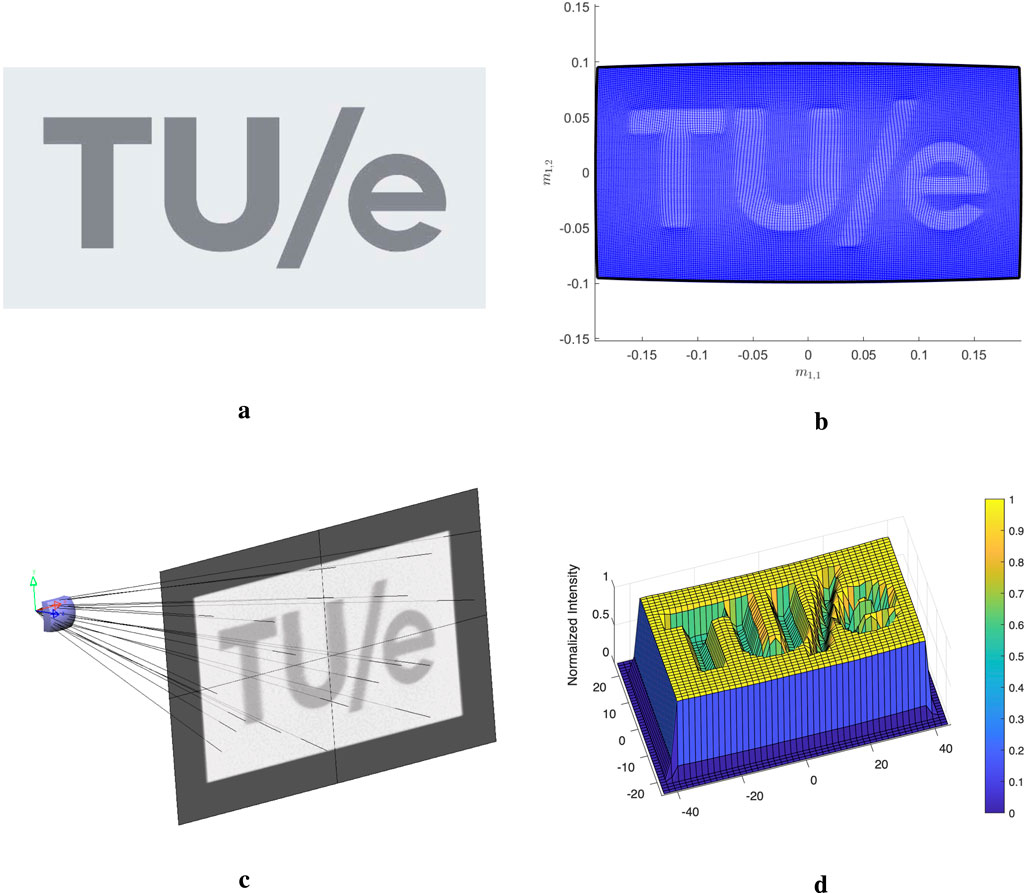For the target, we choose the stereographic domain $\mathcal{Y}=[-0.2,0.2]\times [-0.1,0.1]$ and intensity $I_{\mathrm{t}}(\widehat{\underline{\mathit{t}}}(\mathit{y}))$ corresponding to the gray-scale image of the TU/e logo given in Figure 6a. Both intensities are scaled such that the global luminous flux balance holds, i.e., Equation 35 for $\mathcal{A}=\mathcal{X}$ and $\mathit{m}(\mathcal{A})=\mathcal{Y}$ . Both stereographic coordinates are projections from the south pole; cf. Equation 21. The refractive index of the lens $n=1.5$ , and we enforce a unique solution for the lens surface by setting $u({\mathit{x}}_{\mathrm{c}})=1$ , and therefore, $u_1({\mathit{x}}_{\mathrm{c}})=0$ , corresponding to the central light ray with stereographic source coordinate ${\mathit{x}}_{\mathrm{c}}=\mathit{0}$ and direction vector $\widehat{\underline{\mathit{s}}}({\mathit{x}}_{\mathrm{c}})={\widehat{\underline{\mathit{e}}}}_z$ ; cf. Equation 34b.

Figure 6

Figure 6. Point-to-far-field lens: target intensity pattern, mapping, freeform surface with a ray-traced target intensity pattern, and 3D illuminance distribution of TU/e-logo. (a) TU/e-logo as a target intensity pattern. (b) Mapping displayed in the stereographic projection plane of $\widehat{\underline{\mathit{t}}}$ . (c) Freeform lens and ray-traced target intensity pattern. (d) 3D normalized illuminance distribution, using 50 × 50 bins.

For space discretization of the BVPs in (45) and (46), we cover the source domain with a uniform $201\times 201$ grid and evaluate 500 iterations of scheme (42)–(43), where the associated functionals are defined in Equation 41. We choose $\alpha =10^{-3}$ . The computational time, on a laptop with Intel Core i7 - 11800 H 2.30 GHz processor and a RAM of 16.0 GB, is $443.65$ s (7.39 min). The optical mapping, computed as an image of the source grid, is shown in Figure 6b, and clearly exhibits the TU/e-logo. The computed freeform lens with a ray traced target intensity pattern is shown in Figure 6c. This intensity pattern is computed with the commercial software code LightTools using $5\times 10^6$ rays and clearly resembles the desired intensity. The corresponding (normalized) 3D illuminance distribution, projected on the plane $z=100$ , is shown in Figure 6d.

7.2 Parallel-to-near-field reflector

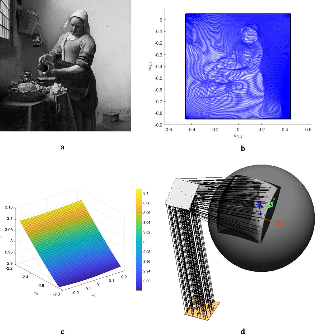
We consider a reflector that converts a uniform source emittance $M(\mathit{x},0)$ into the illuminance $E(\underline{\mathit{r}}(\mathit{y}))$ corresponding to the gray-scale image of the painting ‘the Milkmaid’ by Johannes Vermeer as shown in Figure 7a, projected on a spherical target surface. The source domain $\mathcal{X}=[-0.25,0.25]\times [-2.25,-2.75]$ and the target domain is located on the northern hemisphere of the unit sphere given by $z=v(\mathit{y})=\sqrt{1-|\mathit{y}{|}^2}$ with $\mathcal{Y}=[-0.42,0.42]\times [-0.82,0.02]$ . The parameters $\mathit{x}$ and $\mathit{y}$ are both Cartesian coordinates. The emittance and illuminance are scaled such that the global flux balance holds, i.e., Equation 38 for $\mathcal{A}=\mathcal{X}$ and $\mathit{m}(\mathcal{A})=\mathcal{Y}$ . We enforce a unique solution for the location of the reflector by setting $u({\mathit{x}}_{\mathrm{c}})=u_1({\mathit{x}}_{\mathrm{c}})=3$ , where ${\mathit{x}}_{\mathrm{c}}={(0,-2.5)}^{\mathrm{T}}$ is the center point of the source domain $\mathcal{X}$ .

Figure 7

Figure 7. Parallel-to-near-field reflector: target illuminance pattern, mapping, sag map, and freeform surface with ray-traced target illuminance. (a) “Milkmaid” as target illuminance pattern. (b) Mapping displayed in the orthogonal projection plane of the target surface. (c) Sag map of the freeform reflector. (d) Free-form reflector with ray-traced target illuminance pattern on a sphere.

To discretize the BVPs in Equations 45, 48, we cover the source domain $\mathcal{X}$ with a uniform $201\times 201$ grid and 500 times apply the iteration scheme defined in Equations 49, 43. The associated functionals are defined in Equation 41, where we choose $\alpha =0.05$ , and Equation 47. On the same laptop/processor, the computational time is 496.63 s (8.28 min). The optical map as image of the uniform rectangular source grid is shown in Figure 7b. Clearly, the girl shown in Figure 7a is recognizable in optical mapping as grid points come closer together in regions of high contrast, showing her contours. The sag map of the reflector is shown in Figure 7c.

To verify the reflector computed by the least-squares algorithm, we used LightTools. Implementing the reflector coordinates into this code and specifying the uniformly distributed rectangular source along with the curved target surface, we obtained the reflector system illustrated in Figure 7d, where only 50 rays are shown. The resulting target intensity was obtained tracing $5\times 10^7$ rays. The image of the ‘Milkmaid’ is clearly visible, confirming the validity of the reflector computed by the least-squares algorithm.

8 Concluding remarks

We have presented a systematic and generic derivation of the governing equations for inverse optical design. Using Hamilton’s characteristic functions, we could derive a geometrical equation defining the shape/location of the optical surface(s). From this equation, applying concepts from optimal transport theory, we derived equations for the optical map. To close the model, we presented a generic conservation law of luminous flux. Combining all equations, we derived the luminous flux constraint. Subsequently, we elaborated the generic model in three different models of increasing complexity, on the basis of three example optical systems. We briefly outlined numerical least-squares methods for all models and demonstrated their performance for a few examples.

We intend to expand our research on inverse methods along the following lines. First, we will adjust our numerical methods to incorporate two target distributions; second, we will develop mathematical models and numerical methods for catadioptric systems, where light rays propagate via different paths from the source to target, and finally, and probably the most challenging, we intent to generalize our models and numerics to optical systems with finite sources, as opposed to zero-étendue sources.

Data availability statement

The original contributions presented in the study are included in the article/Supplementary Material; further inquiries can be directed to the corresponding author.

Author contributions

JT: writing–original draft and writing–review and editing. KM: writing–original draft and writing–review and editing. MA: writing–review and editing. LK: writing–review and editing. PB: writing–review and editing. WI: writing–review and editing.

Funding

The author(s) declare that financial support was received for the research, authorship, and/or publication of this article. This work was partially supported by the Dutch Research Council (Dutch: Nederlandse Organisatie voor Wetenschappelijk Onderzoek–NWO) through the (grants P15-36 and P21-20).

Acknowledgments

The authors would like to thank R. Beltman from Signify for executing all LightTools simulations.

Conflict of interest

The authors declare that the research was conducted in the absence of any commercial or financial relationships that could be construed as a potential conflict of interest.

Generative AI statement

The author(s) declare that no Generative AI was used in the creation of this manuscript.

Publisher’s note

All claims expressed in this article are solely those of the authors and do not necessarily represent those of their affiliated organizations, or those of the publisher, the editors and the reviewers. Any product that may be evaluated in this article, or claim that may be made by its manufacturer, is not guaranteed or endorsed by the publisher.

References

1. Filosa C. Phase space ray tracing for illumination optics. Eindhoven: Eindhoven University of Technology (2018). PhD Thesis.

Google Scholar

2. Santambrogio F. Optimal transport for applied mathematicians. Birkäuser, New York: Springer (2015).

Google Scholar

3. Gutiérrez C. The Monge-Ampère equation. 2nd ed. Switzerland: Birkhäuser: Springer International Publishing AG (2016).

Google Scholar

4. Romijn L. Generated Jacobian equations in freeform optical design. Eindhoven: Eindhoven University of Technology (2021). PhD Thesis.

Google Scholar

5. Froese B. A numerical method for the elliptic Monge–Ampère equation with transport boundary conditions. SIAM J Scientific Comput (2012) 34:A1432–59. doi:10.1137/110822372

CrossRef Full Text | Google Scholar

6. Benamou J, Froese B, Oberman A. Numerical solution of the optimal transportation problem using the Monge–Ampère equation. J Comput Phys (2014) 260:107–26. doi:10.1016/j.jcp.2013.12.015

CrossRef Full Text | Google Scholar

7. Kawecki E, Lakkis O, Pryer T. A finite element method for the Monge-Ampère equation with transport boundary conditions. arXiv preprint arXiv:1807 (2018).

Google Scholar

8. Caffarelli L, Oliker V. Weak solutions of one inverse problem in geometric optics. J Math Sci (2008) 154:39–49. doi:10.1007/s10958-008-9152-x

CrossRef Full Text | Google Scholar

9. Kitagawa J, Mérigot Q, Thibert B. Convergence of a Newton algorithm for semi-discrete optimal transport. J Eur Math Soc (2019) 21:2603–51. doi:10.4171/jems/889

CrossRef Full Text | Google Scholar

10. Mérigot Q, Thibert B. Mirrors, lenses and Monge-Ampère equations. Eur Math Soc Mag (2021) 120:16–28. doi:10.4171/mag-21

CrossRef Full Text | Google Scholar

11. Gallouet A, Mérigot Q, Thibert B. A damped Newton algorithm for generated Jacobian equations. Calculus of Variations and Partial Differential Equations (2021) 61:49–59. doi:10.1007/s00526-021-02147-7

CrossRef Full Text | Google Scholar

12. Caboussat A, Glowinski R, Sorensen D. A least-squares method for the numerical solution of the Dirichlet problem for the elliptic Monge − Ampère equation in dimension two. ESAIM: Control, Optimisation and Calculus of Variations (2013) 19:780–810. doi:10.1051/cocv/2012033

CrossRef Full Text | Google Scholar

13. Prins C, Beltman R, ten Thije Boonkkamp J, IJzerman W, Tukker T. A least-squares method for optimal transport using the Monge-Ampère equation. SIAM J Scientific Comput (2015) 37:B937–61. doi:10.1137/140986414

CrossRef Full Text | Google Scholar

14. Yadav N, ten Thije Boonkkamp J, IJzerman W. A Monge-Ampère problem with non-quadratic cost function to compute freeform lens surfaces. J Sci Comput (2019) 80:475–99. doi:10.1007/s10915-019-00948-9

CrossRef Full Text | Google Scholar

15. Romijn L, ten Thije Boonkkamp J, IJzerman W. Freeform lens design for a point source and far-field target. J Opt Soc Am A (2019) 36:1926–39. doi:10.1364/josaa.36.001926

PubMed Abstract | CrossRef Full Text | Google Scholar

16. Romijn L, ten Thije Boonkkamp J, IJzerman W. Inverse reflector design for a point source and far-field target. J Comput Phys (2020) 408:109283. doi:10.1016/j.jcp.2020.109283

CrossRef Full Text | Google Scholar

17. Romijn L, Anthonissen M, ten Thije Boonkkamp J, IJzerman W. The generating function approach for double freeform lens design. J Opt Soc Am A (2021) 38:356–68. doi:10.1364/OE.438920

PubMed Abstract | CrossRef Full Text | Google Scholar

18. Romijn L, ten Thije Boonkkamp J, Anthonissen M, IJzerman W. An iterative least-squares method for generated Jacobian equations in freeform optical design. SIAM J Scientific Comput (2021) 43:B298–B322. doi:10.1364/OE.438920

CrossRef Full Text | Google Scholar

19. Luneburg R. Mathematical theory of optics. Berkeley and Los Angeles: University of California Press (1966).

Google Scholar

20. Born M, Wolf E. Principles of optics: electromagnetic theory of propagation, interference and diffraction of light. 5th ed. Oxford: Pergamon Press (1975).

Google Scholar

21. Kevorkian J. Partial differential equations: analytical solution techniques. Pacific Grove, California: Brooks/Cole (1990).

Google Scholar

22. Guillen N. A primer on generated Jacobian equations: geometry, optics, economics. Notices Am Math Soc (2019) 66:1401–11. doi:10.1090/noti1956

CrossRef Full Text | Google Scholar

23. Yadav N. Monge-Ampère problems with non-quadratic cost function: application to freeform optics. Eindhoven: Eindhoven University of Technology (2018). PhD Thesis.

Google Scholar

24. Ries H, Rable A. Edge-ray principle of nonimaging optics. J Opt Soc Am A (2002) 19:590–5. doi:10.1364/OE.438920

CrossRef Full Text | Google Scholar

25. Chaves J. Introduction to nonimaging optics. 2nd ed. Boca Raton, Florida: CRC Press (2016).

CrossRef Full Text | Google Scholar

26. Anthonissen M, ten Thije Boonkkamp J, IJzerman W. Unified mathematical framework for a class of fundamental freeform optical systems. Opt Express (2021) 29:31650–64. doi:10.1364/OE.438920

PubMed Abstract | CrossRef Full Text | Google Scholar

27. Prins C. Inverse methods for illumination optics. Eindhoven: Eindhoven University of Technology (2014). PhD Thesis.

Google Scholar

28. Beltman R, ten Thije Boonkkamp J, IJzerman W. A least-squares method for the inverse reflector problem in arbitrary orthogonal coordinates. J Comput Phys (2018) 367:347–73. doi:10.1016/j.jcp.2018.04.041

CrossRef Full Text | Google Scholar

29. Yadav N, Romijn L, ten Thije Boonkkamp J, IJzerman W. A least-squares method for the design of two-reflector optical systems. J Phys Photon (2019) 1:034001. doi:10.1088/2515-7647/ab2db3

CrossRef Full Text | Google Scholar

30. Courant R, Hilbert D. Methods of mathematical physics, 2. New York: John Wiley and Sons (1989). doi:10.1002/9783527617210

CrossRef Full Text | Google Scholar

31. Wang C, Luo Y, Li H, Zang Z, Xu Y, Han Y, et al. Extended ray-mapping method based on differentiable ray-tracing for non-paraxial and off-axis freeform illumination lens design. Optics Express (2023) 31:30066–30078.

PubMed Abstract | CrossRef Full Text | Google Scholar

32. Heemels A, de Koning B, Möller M, Adam A. Optimizing freeform lenses for extended sources with algorithmic differentiable ray tracing and truncated hierarchical B-splines. Optics Express (2024) 32:9730–9746.

PubMed Abstract | CrossRef Full Text | Google Scholar

33. Doskolovich L, Bykov D, Andreev E, Bezus E, Oliker V. Designing double freeform surfaces for collimated beam shaping with optimal mass transportation and linear assignment problems. Optics Express (2018) 26:24602–24613.

PubMed Abstract | CrossRef Full Text | Google Scholar

34. Doskolovich L, Bykov D, Mingazov A, Bezus E. Optimal mass transportation and linear assignment problems in the design of freeform refractive optical elements generating far-field irradiance distributions. Optics Express (2019) 27:13083–13097.

PubMed Abstract | CrossRef Full Text | Google Scholar

35. Brix K, Hafizogullari Y, Platen A. Designing illumination lenses and mirrors by the numerical solution of Monge-Ampère equations. J Opt Soc Am A (2015) 32:2227–2236.

PubMed Abstract | CrossRef Full Text | Google Scholar

36. Feng Z, Froese B, Liang R. Freeform illumination optics construction following an optimal transport map. Appl. Optics (2016) 55:4301–4306.

PubMed Abstract | CrossRef Full Text | Google Scholar

37. Bösel C, Gross H. Single freeform surface design for prescribed input wavefront and target irradiance. J Opt Soc Am (2017) 34:1490–1499.

PubMed Abstract | CrossRef Full Text | Google Scholar

38. Bösel C, Gross H. Double freeform illumination design for prescribed wavefronts and irradiances. J Opt Soc Am (2017) 35:236–243.

PubMed Abstract | CrossRef Full Text | Google Scholar

Nomenclature

Scalar variables

$\mathit{c}(\mathit{x},\mathit{y})$ cost function

$\mathit{d}(\mathbf{P},\mathbf{Q})$ distance between the points $\mathbf{P}$ and $\mathbf{Q}$

${\mathit{d}}_{\mathbf{opt}}({\underline{\mathit{r}}}_{\mathbf{s}},{\underline{\mathit{r}}}_{\mathbf{t}})$ optical distance, i.e., optical path length $[{\mathbf{P}}_{\mathbf{s}},{\mathbf{P}}_{\mathbf{t}}]$ as function of the position vectors ${\underline{\mathit{r}}}_{\mathbf{s}}$ and ${\underline{\mathit{r}}}_{\mathbf{t}}$

$\mathit{E}(\underline{\mathit{r}}(\mathit{y}))$ illuminance at a near-field target

$\mathit{f}(\mathit{x})$ generic flux density of the source

$\mathit{g}(\mathit{y})$ generic flux density of the target

$\mathit{G}(\mathit{x},\mathit{y},\mathit{w})$ generating function

$\mathit{H}(\mathit{x},\mathit{y},\mathit{w})$ inverse of generating function

${\mathit{I}}_{\mathbf{s}}(\widehat{\underline{\mathit{s}}}(\mathit{x}))$ intensity of the point source

${\mathit{I}}_{\mathbf{t}}(\widehat{\underline{\mathit{t}}}(\mathit{y}))$ intensity of the far-field target

$\mathit{J}(\widehat{\underline{\mathit{v}}}(\mathit{z}))$ factor in the area element $\mathrm{d}S(\mathit{z})$ on ${\mathrm{S}}^2$ generated by $\widehat{\underline{\mathit{v}}}$ and parameterized by $\mathit{z}$

$\mathit{M}(\underline{\mathit{r}}(\mathit{x}))$ emittance of the planar source

$\mathit{n}(\underline{\mathit{r}})$ refractive index field

$\mathit{s}$ arc length along a curve $\mathcal{C}$ representing a ray

$\mathit{T}({\mathit{p}}_{\mathbf{s}},{\mathit{p}}_{\mathbf{t}})$ angular characteristic (function)

${\mathit{u}}_{\mathit{1}}(\mathit{x})$ Kantorovich potential for source domain

${\mathit{u}}_{\mathit{2}}(\mathit{y})$ Kantorovich potential for target domain

$\mathit{V}({\mathit{q}}_{\mathbf{s}},{\mathit{q}}_{\mathbf{t}})$ point characteristic (function)

$\mathit{W}({\mathit{q}}_{\mathbf{s}},{\mathit{p}}_{\mathbf{t}})$ mixed characteristic (function) of the first kind

${\mathit{W}}^{*}({\mathit{p}}_{\mathbf{s}},{\mathit{q}}_{\mathbf{t}})$ mixed characteristic (function) of the second kind

$\mathit{z}$ coordinate along the optical axis

$\mathit{\phi }(\underline{\mathit{r}})$ phase of an electromagnetic wave

$[{\mathbf{P}}_{\mathbf{s}},{\mathbf{P}}_{\mathbf{t}}]$ optical path length between the points ${\mathrm{P}}_{\mathrm{s}}$ and ${\mathrm{P}}_{\mathrm{t}}$

Vectors

$\mathit{p}(\mathit{z})$ 2D momentum vector of a ray

$\mathit{q}(\mathit{z})$ 2D position vector of a ray

$\underline{\mathit{r}}$ 3D position vector of an arbitrary point

$\widehat{\underline{\mathit{s}}}$ 3D unit direction/tangent vector of a ray at the source plane

$\widehat{\underline{\mathit{t}}}$ 3D unit direction/tangent vector of a ray at the target plane

$\widehat{\underline{\mathit{v}}}$ 3D unit direction/tangent vector at an arbitrary point of a ray

$\mathit{x}$ 2D vector parameterizing the source domain

$\mathit{y}$ 2D vector parameterizing the target domain