Prediction of thermospheric temperature over the South Pole based on two-layer LSTM network

This study presents a new two-layer LSTM network-based model, which improves the accuracy of thermospheric temperature over the South Pole simulated by MSIS2.0 model. A dataset is constructed using temperature data measured by the South Pole FPI from 2000 to 2011 along with corresponding temperature derived from MSIS2.0 model, F10.7 and Ap indices, which are the input parameters of the first LSTM network layer. The first LSTM layer combines these inputs into a one-dimensional time series, while the second LSTM layer extracts temporal features from the output of the first layer. The proposed LSTM-based model shows better performance in predicting FPI observations compared to the empirical MSIS2.0 model during both geomagnetically quiet and disturbed periods. For the year 2011, the mean absolute error between the MSIS2.0 model and FPI data is 53.460 K, whereas the LSTM model reduces it to 34.024 K. The euclidean distance analysis also demonstrates better performance of the LSTM model. This study illustrates the potential of applying a two-layer LSTM network to optimize model simulations in upper atmosphere research.

1 Introduction

The Earth’s atmosphere is a complex system that plays a vital role in regulating climate and sustaining life. Understanding the interactions between the Earth and space, particularly in the upper atmosphere spanning from 80 km to 500 km, holds great importance [1]. Extensive researches have been conducted over several decades to help our understanding of this region [2].

Fabry-Perot Interferometer (FPI [3]) instruments measure temperature and wind velocity in the upper atmosphere based on doppler shifts observed in transmitted light. Only a limited number of FPIs have been deployed in the South Pole region to study the temporal evolution of thermospheric parameters [4, 5]. Given the limited observational data available, researchers have conducted a series of studies on the phenomena of winds and temperatures over polar regions under conditions of solar activity and geomagnetic activity[6–8]. To enhance these investigations, additional observational data are often required, including data from balloon [9] and satellite [10] observations.Furthermore, temperature data observation based on FPI is lack of data during the beginning and end of each year. For example, observations of temperature data over the South Pole often exhibit data gaps [11].

To address this shortcoming, numerical simulation work can be employed. Models such as DTM (Dynamic Thermosphere Model [12, 13]), TIEGCM (Thermosphere-Ionosphere-Electrodynamics General Circulation Model, [14]), and GITM (Global Ionosphere-Thermosphere Model, [15]) can provide continuous temporal variations at a particular location and address the problem of gap.Among various models used for simulating the upper atmosphere, the Mass Spectrometer Incoherent Scatter (MSIS) model stands out as one of the most widely employed ([16]). The MSIS model combines theory and observations to predict upper atmospheric behavior, providing valuable insights into composition, density, temperature, and other properties [17, 18]. Despite its effectiveness, there are limitations associated with the MSIS model that need improvements for more accurate predictions.The MSIS model family has been continuously evolving and improving since the early 1970s. Accurate prediction of FPI values from MSIS simulations poses challenges due to inherent complexities and dynamic nature within these regions. It necessitates precise modeling of multiple physical processes involving ion-neutral interactions, chemical reactions, and energy transfer mechanisms. Advanced techniques are required to optimize MSIS simulations effectively while improving FPI value prediction accuracy.Recently, Licata et al. [19] developed a machine learning-based MSIS-UQ model and calibrated it against NRLMSIS2.0 to reduce the discrepancies between the model and satellite density. The research findings show that MSIS-UQ achieved significant improvement in terms of MAE (Mean Absolute Error) compared to NRLMSIS2.0, reducing the differences between the model and satellite density by approximately 25% [19]. It outperformed the High Accuracy Satellite Drag Model (HASDM) by approximately 11% [21].

Although these models can compensate for gaps in observational data, the discrepancies between the simulation results and the actual observations remain significant. For instance, Huang et al. [22] demonstrates that the neutral temperature at Palmer Station during geomagnetic storms simulated from TIEGCM is much smaller to the FPI observations.Similarly, Lee et al. [5] reveals that the observed temperature in the upper atmosphere at Jang Bogo Station (JBS) in Antarctica is approximately 200 K higher than the simulated results from TIEGCM during geomagnetic storms.

We propose a novel approach utilizing a two-layer Long Short-Term Memory (LSTM) network [23, 24] framework to optimize MSIS2.0 simulation results over Antarctica.LSTM networks, which are designed to handle sequential data while retaining long-term dependencies, are well-suited for processing time-series data, making them promising tools for improving atmospheric simulations [25]. Reddybattula et al. [26] developed an LSTM-based model using 8 years of GPS-TEC data to forecast ionospheric total electron content at a low-latitude Indian station, outperforming traditional models like IRI-2016. Similarly, Vankadara et al. [27] proposed a Bi-LSTM model trained on 11 months of TEC data with solar and geomagnetic indices, which accurately forecasts ionospheric total electron content and surpasses conventional models such as LSTM, ARIMA, IRI-2020, and GIM. More studies have explored the application of LSTM networks in atmospheric data processing, including researches by Hao et al. [28]; Kun et al. [29]. These investigations specifically highlight the remarkable achievements of LSTM networks in the domain of atmospheric prediction. They underscore the exceptional capabilities of LSTM networks in effectively processing atmospheric data and significantly improving prediction accuracy for atmospheric forecasting [30, 31]. In addition, Zhang et al. [32] confirmed that, compared to traditional neural network models, the combination of models and neural networks with applied physical constraints have greater potential in space weather applications. The two-layer LSTM network constructed in this work is not a conventional LSTM network. On one hand, it is composed of two independent LSTM networks; on the other, the functions implemented by these two networks are different. However, LSTM networks have been widely applied in prediction problems, there has been relatively limited research on their application in handling regression problems. Therefore, it is crucial to explore and investigate the potential of LSTM networks in addressing regression problems.

In this study, we use FPI-measured temperature at South Pole from year 2000–2011 to train a two-layer LSTM network in order to develop a prediction model. It presents a promising avenue for improving the overall accuracy predicting FPI measurements, contributing to better understanding of upper atmospheric dynamics through advanced neural networks.

2 Data and models

2.1 Neutral temperature measured by FPI at the South Pole

The thermospheric temperature measured by FPI at the South Pole from 2000 to 2011 is used in this study, sourced from Madrigal database (https://cedar.openmadrigal.org/list). Figure 1 shows temporal variation of the neural temperature at 250 km between Day of Year (DOY) 100 and 245 from year 2000–2011. The black line represents the measurements overlapped over the 11 years, whereas the red line depicts the averaged temperature for these years. Figure 2 shows the temporal distribution of temperature data counts, with a total number of about 400,000 counts from year 2000–2011. The top panel displays the hourly distribution of temperature data, which is relatively uniform. The middle panel presents monthly data counts, with the fewest in September, exceeding 10,000. It is worth noting that FPI observations begin in April and end around September every year. The bottom panel shows the data counts for each year, with the least count in year 2003.

Figure 1

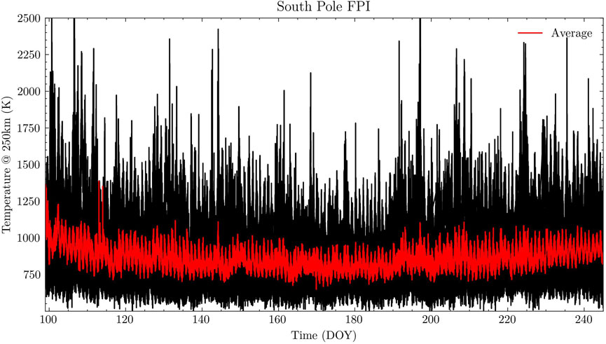
Figure 1. Thermospheric temperature at 250 km measured by the South Pole FPI from year 2000–2011. The black lines represents the temporal variation of overlapped temperatures from DOY 100 to DOY 245, while the red line is the average over these 11 years.

Figure 2

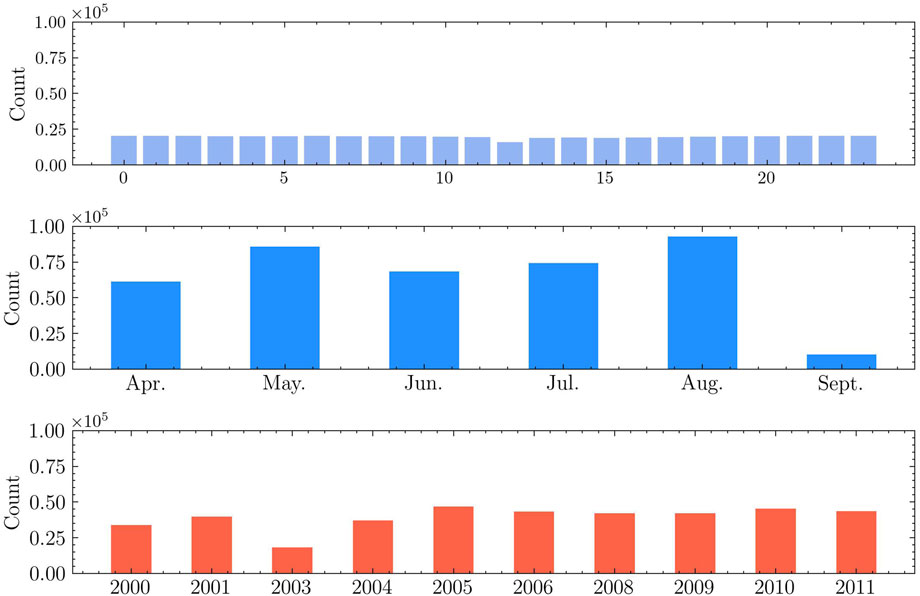
Figure 2. Local time (upper panel), Monthly (middle panel) and annual (bottom panel) distribution of the South Pole FPI data counts.

The FPI temperature measurements exhibit a mean absolute error of 34.31 K (the temperature range spans approximately 500–3000 K), with a mean relative error of 3.91% and a median relative error of 3.37%. The proportion of errors greater than 100 K is 1.75%, and the proportion of errors greater than 200 K is 0.07%. The standard deviation of 2.24% suggests that the measurement noise is constrained but non-negligible, particularly given the dynamic range of the thermosphere. Observational error and abrupt fluctuations in FPI data hinder neural networks from effectively extracting time series features. To address this challenge, we employed a Savitzky-Golay filter [33] with a 3-h temporal window. This approach leverages localized polynomial regression to adaptively smooth noise while preserving the integrity of transient features. The Savitzky-Golay filter smooths data by fitting a polynomial within a moving window, with its core operation defined by the Equation 1.

$y_i^{\text{smoothed}}={\displaystyle \sum _{j=-m}^m}{c}_j{y}_{i+j}(1)$

where $y_{i+j}$ represents the data within a window of $2m+1$ points centered around $y_i$, and $c_j$ are the filter coefficients obtained by fitting a polynomial of degree $n$ (with $n<2m+1$) through least squares regression. This equation shows that each smoothed value is a weighted sum of the surrounding data points. The coefficients $c_j$ are designed to reduce noise while preserving important signal features. In this study, the smoothing time window was set to 3 h based on two considerations. First, a large window would reduce the differences between extreme values, whereas a too small window would not reduce noise, and an empirically determined 3 h serves as a suitable compromise. Additionally, since the MSIS2.0 simulation is based on AP and F10.7 data, with a time resolution matching the lower-resolution AP data (3 h), the smoothing window was set to 3 h.

2.2 Temperature simulated by the MSIS2.0 model

In this study, the MSIS2.0 model (referred to as MSIS) is used, which is an empirical atmospheric model that describes the average observed behaviors of temperature and mass density through a parametric analytic formulation [34]. The model inputs include location, time, solar activity F10.7 index and geomagnetic activity Ap index [35], sourced from the OMNI database (https://omniweb.gsfc.nasa.gov/ow.html). The F10.7 index measures solar radiation intensity at a wavelength of 10.7 cm and is used to assess solar activity’s impact on the Earth’s atmosphere, especially in the thermosphere and ionosphere.The AP index quantifies the activity level of the Earth’s magnetic field based on measurements from multiple ground stations. It reflects the intensity of interactions between solar wind and the Earth’s magnetic field. The temporal resolution of AP index is 3 h, while that of F10.7 index is 1 day. To ensure consistency, the F10.7 and Ap indices were upsampled via linear interpolation to match the FPI timestamps, which have a resolution of approximately 3 min, before running the MSIS simulations and model training.

The MSIS model is employed to simulate the neutral temperature at an altitude of 250 km at the South Pole for the period from 2000 to 2011. Figure 3 depicts the MSIS simulated temperatures similar to Figure 1. The blue line in Figure 3 also illustrates a seasonal variation with lowest temperature in winters at the South Pole.

Figure 3

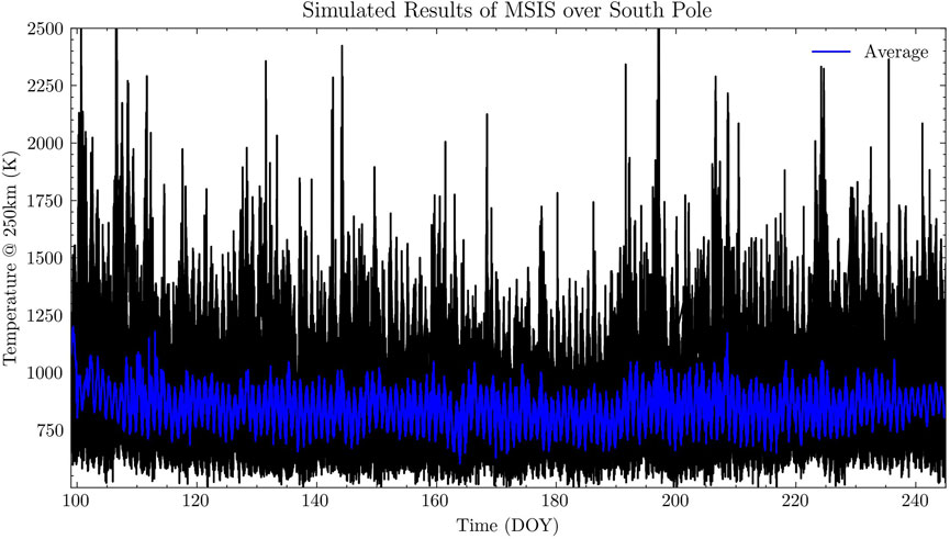
Figure 3. Thermospheric temperature at 250 km simulated by MSIS from year 2000–2011. The black lines represents the temporal variation of overlapped temperature, while the blue line is the average value over these 11 years.

2.3 Development of temperature prediction model based on two-layer LSTM network

A dataset is constructed using FPI data as the label and the corresponding MSIS simulations, F10.7, and Ap indices as the features, all aligned with the FPI observational timeline. In the training process of neural networks, the data is typically divided into three categories: training set, validation set and test set. The training set is the data used to train the model and to enable the model to learn the relationship between features and labels. Validation Set is the data used to evaluate the model’s generalization ability during training and help prevent overfitting, and it is also used for tuning model hyperparameters or selecting the best model. The test set is the data used for the final evaluation of model performance on new data after training. The data from 2000 to 2009 is used to train the LSTM network, while the data from 2010 is used for cross-validation during the training process. The MAE between the model and the FPI for 2010 is calculated, and if it exceeds the MAE between the MSIS and the FPI for three consecutive epochs, training will stop. The data from 2011 is used to test the performance of the trained network.

The LSTM network is a powerful neural architecture that effectively manages information input and output through gating mechanisms (including input gate, output gate, and forget gate [36]), as depicted in Figure 4. As a Recurrent Neural Network (RNN) specifically designed for sequential data processing, such as text data in natural language processing, the LSTM network excels at controlling information flow and addressing issues like gradient vanishing during deep training [37]. The flow of information in an LSTM can be summarized as follows: the forget gate, the input gate, the cell state, and the output gate.

Figure 4

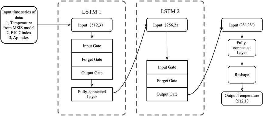
Figure 4. Two-layer LSTM network Diagram.

The forget gate $f_t$ determines how much historical information to retain from the cell state using a sigmoid function $\sigma$ [38]. As shown in Equation 2, it combines the previous hidden state $h^{⟨t-1⟩}$ and current input $x^{⟨t⟩}$, $W_f$ is a weight matrix partitioned into $W_{fh}$ (for $h^{⟨t-1⟩}$) and $W_{fx}$ (for $x^{⟨t⟩}$), which are learned independently. $b_f$ is the bias term, and $\sigma$ scales outputs to [0,1], representing retention probabilities.

$f_t=\sigma \left(W_f\cdot \left[h^{\langle t-1\rangle },x^{\langle t\rangle }\right]+b_f\right)(2)$

The input gate determines which new information should be stored in the cell state, and it is composed of two components, a sigmoid layer that decides which information should be updated and a tanh layer that generates new candidate values of the cell state ${\tilde{c}}^{⟨t⟩}$, as shown in Equations 3, 4, $W_c$ and $W_i$ is a weight matrix, $b_i$ and $b_c$ is the bias term, the Tanh function compresses the input to a specific range (−1, 1), helping to stabilize the network by preventing excessively large or small values.

$i_t=\sigma \left(W_i\cdot \left[h^{\langle t-1\rangle },x^{\langle t\rangle }\right]+b_i\right)(3)$

${\tilde{c}}^{⟨t⟩}=Tanh\left(W_c\cdot \left[h^{⟨t-1⟩},x^{⟨t⟩}\right]+b_c\right)(4)$

The cell state $c^{⟨t⟩}$ is updated by combining the forget gate and the input gate, as expressed by the Equation 5, where $c^{⟨t⟩}$ is the cell state at the current time step and $c^{⟨t-1⟩}$ is the cell state from the previous time step. The term $f_t\ast c^{⟨t-1⟩}$ indicates the old information retained by the forget gate, while $i_t\ast {\tilde{c}}^{⟨t⟩}$ represents the new information added by the input gate.

$c^{⟨t⟩}=f_t\ast c^{⟨t-1⟩}+i_t\ast {\tilde{c}}^{⟨t⟩}(5)$

The output gate determines the hidden state $h^{⟨t⟩}$ at the current time step. It controls the output using a sigmoid function that decides which parts of the cell state should be output and a tanh function that scales the cell state values, as shown in Equations 6, 7.

$o_t=\sigma \left(W_o\cdot \left[h^{\langle t-1\rangle },x^{\langle t\rangle }\right]+b_o\right)(6)$

$h^{\langle t\rangle }=o_t\ast \tanh \left(c^{\langle t\rangle }\right)(7)$

We designed a two-layer LSTM network where each layer serves a different function (see Figure 4). Table 1 presents the hyperparameters associated with our chosen LSTM network structure. The first LSTM layer (a single-layer LSTM) processes the input data, which consists of MSIS-derived temperatures, F10.7, and Ap indices, arranged as a time series of length 512 with 3 features [i.e., shape (512, 3)]. This LSTM layer with 256 hidden units outputs a transformed sequence, resulting in a shape of (512, 256). A fully connected layer is then applied to reduce this output to a one-dimensional series, yielding a shape of (512, 1). Essentially, this process combines three features into one feature. A standard fully connected network (without LSTM) can also merge features, but it only processes the current time step. We use an LSTM because it integrates information from neighboring time steps [37], capturing the temporal dependencies in the data. Before feeding this output into the second LSTM layer, it is reshaped from (512, 1) to (256, 2) because the original data often shows significant differences between consecutive time points; by merging every two time steps into one, the training process becomes more stable. The second LSTM layer (a four-layer LSTM) takes the reshaped input (256, 2) and extracts higher-level features, producing an output of shape (256, 256). A fully connected layer then processes this output, initially reformatting it to (256, 2) before reshaping it to restore the original sequence length (512, 1). In summary, the first LSTM layer reduces dimensionality, the second LSTM layer captures high-level patterns, and the final fully connected layer restores the sequence length.

Table 1

Table 1. The essential hyperparameters of the two-layer LSTM.

In predictive applications using LSTM networks, it is common to retain only the final timestep output as the forecast [39]. For example, when the LSTM output shape is (10,5), indicating 10 timesteps with 5 features, it retains the five features from the final timestep (shape 1,5) as the prediction for the 11th timestep. In contrast, our regression model retains all output information and uses it to fully reconstruct a time series of the same length as the input.

3 Validation of the LSTM-Network based model

The two-layer LSTM model aims to improve the prediction accuracy of the MSIS model. To validate this, two critical aspects require verification, the one is whether this model improves the accuracy compared to its baseline, the other is whether it outperforms existing models under identical experimental conditions.

Firstly, we have verified whether the model enhances the prediction accuracy of the MSIS model by analyzing two aspects: testing its performance during both quiet periods and geomagnetic storm events, and evaluating it across the entire test dataset. As shown in Figure 5, during the quiet time from DOY 176 to 182 in year 2011, there are little variation in Interplanetary Magnetic Field (IMF) $B_z$, dynamic pressure of the solar wind (Pd), Ap index, F10.7 index and Dst index, while during the storm time from DOY 145 to 153, there were obvious disturbances in IMF, Pd, and Dst indices. The results of temperature at 250 km over the South Pole for both quiet time (left) and storm time (right) are shown in Figure 6. The first row displays the Dst index variation. The second row compares observed thermospheric temperature (South Pole FPI, smoothed) with MSIS simulations and two-layer LSTM result. The third and fourth rows show absolute and percentage differences between models and observations. To quantify these discrepancies, MAE and MAPE (Mean Absolute Percentage Error) are calculated using Equations 8, 9, where $y_i$ denotes the observed values and ${\widehat{y}}_i$ represents the model predictions.

$\text{MAE}=\frac{1}{n}{\displaystyle \sum _{i=1}^n}|y_i-{\widehat{y}}_i|(8)$

$\text{MAPE}\left(\%\right)=\frac{100}{n}{\displaystyle \sum _{i=1}^n}\left|\frac{y_i-{\widehat{y}}_i}{y_i}\right|(9)$

Figure 5

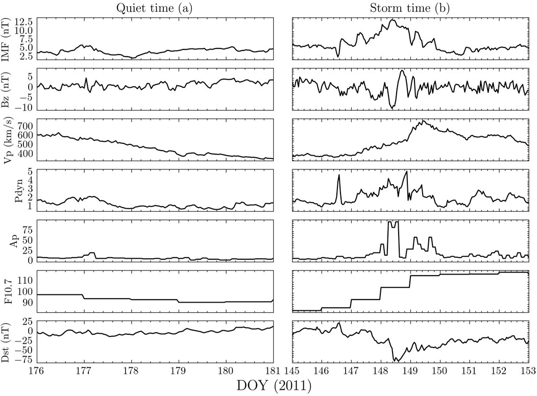
Figure 5. Temporal variation of solar and geomagnetic conditions during two selected periods, the quiet time from DOY 176 to 182 in year 2011 on the left, the storm time from DOY 216 to 221 on the right. From top to bottom panels they are total IMF magnetic field, IMF component in the z-direction $B_z$, solar wind speed, solar wind dynamic pressure, Ap, F10.7 and Dst indices. (a) Quiet time (b) storm time.

Figure 6

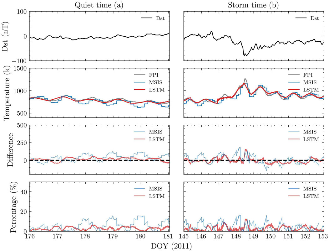
Figure 6. Comparison of the temporal variations at the South Pole during the quiet (left) and storm (right) time. From top to bottom panels are the Dst index, temperature measured by the South Pole FPI (black) and those simulated by the MSIS model (blue) and our two-layer LSTM model (red), differences between the model results and the observation, and their percentage differences. (a) Quiet time (b) storm time.

Further calculations during quiet periods reveal that the MAE between MSIS model and FPI measurement is 49.40 K, while that between LSTM model and FPI data is 23.37 K. The MAPE between MSIS model and FPI measurement is 6.36%, compared to 2.95% for the LSTM model. During the geomagnetic storm time, the MSIS model having a MAE of 47.56 K and a MAPE of 5.39%, and the LSTM model showing a MAE of 26.29 K and a MAPE of 2.92%. For the entire test dataset (all data of year 2011), the MAE between MSIS model and FPI data is 53.46 K, while the MAE of LSTM model is 34.02 K, the MAPE between MSIS model and FPI measurement is 6.12%, compared to 3.82% for the LSTM model. These results demonstrate that both MSIS model and LSTM based Model do well predicting the thermospheric temperature at the South Pole, and the LSTM model improves the forecasting performance by approximately 15 K compared to the MSIS model.

Secondly, we validate whether the two-layer LSTM model outperforms existing models. Under the same conditions, we added simulation results from the DTM model and the one-layer LSTM, and introduced two metrics, RMSE (Root Mean Square Error) and $R^2$ (Coefficient of Determination), for validation. These two metrics are shown in Equations 10, 11. Table 2 shows performance metrics calculated from comparing the model results with the smoothed observational data. $R^2$ indicates how well the model’s predictions match the data (closer to 1 is better), MAE gives the average error, RMSE emphasizes larger errors, and MAPE shows the error as a percentage. By comparing these metrics, the two-layer LSTM network outperforms the other models on all four indicators. It shows the smallest error relative to the raw data and the greatest improvement in MSIS model performance.

$\text{RMSE}=\sqrt{\frac{1}{n}{\displaystyle \sum _{i=1}^n}{\left(y_i-{\widehat{y}}_i\right)}^2}(10)$

$R^2=1-\frac{{\sum }_{i=1}^n{\left(y_i-{\widehat{y}}_i\right)}^2}{{\sum }_{i=1}^n{\left(y_i-\bar{y}\right)}^2}(11)$

Table 2

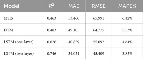
Table 2. Performance comparison between two-layer LSTM and baseline models for the whole year of 2011.

To clearly show the error distribution of these models on the entire test set, we used kernel density estimation to plot their Euclidean distance error distribution, as shown in Figure 7. For the Euclidean distance, we first divided the test set into daily segments and then calculated the Euclidean distance for each segment, the calculation method for the Euclidean distance is given in Equation 12, $y_i$ represents the model values, and ${\widehat{y}}_i$ represents the observed values. The Euclidean distance for time series is a method used to measure the similarity or dissimilarity between two time series [40]. It calculates the difference between corresponding values of the two time series at each time point, squares these differences, sums them up, and takes the square root of the total to obtain the final distance. In simple terms, Euclidean distance measures the straight-line distance between numerical values of two time series at each time point. A smaller Euclidean distance indicates that the two time series are closer or more similar to each other, while a larger Euclidean distance suggests they are farther apart or have greater differences. Kernel density estimation uses a smoothing kernel to estimate the probability density function of data. Equation 13 shows that $\widehat{f}(x)$ is the estimated density function, where $n$ is the number of data points, $h$ is the smoothing bandwidth, and $K(\cdot )$ is the kernel function. Here, $x_i$ represents the Euclidean distances with the square root $\sqrt{d}$, and $x$ is the Euclidean distance at which the density is estimated.

$d=\sqrt{{\displaystyle \sum _{i=1}^n}{\left(y_i-{\widehat{y}}_i\right)}^2}(12)$

$\widehat{f}\left(x\right)=\frac{1}{nh}{\displaystyle \sum _{i=1}^n}K\left(\frac{x-x_i}{h}\right)(13)$

Figure 7

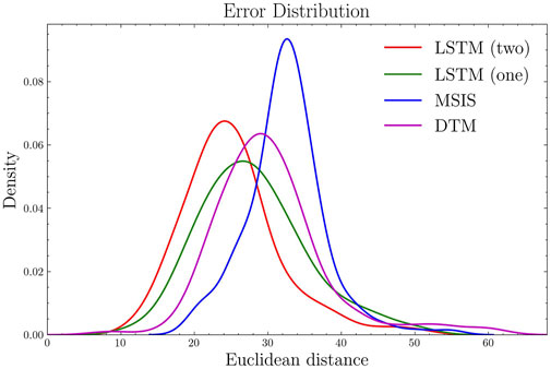
Figure 7. The results of kernel density estimation for the euclidean distance between models and FPI observations.

Figure 7 shows the Euclidean distances between model results and FPI measurements using kernel density estimation. The blue line represents MSIS, the yellow line represents DTM, the red line represents the two-layer LSTM, and the green line represents the one-layer LSTM. The peak values are (32.678, 0.094) for MSIS, (28.959, 0.064) for DTM, (26.638, 0.055) for the one-layer LSTM, and (24.109, 0.068) for the two-layer LSTM. These peaks represent the most frequent error magnitudes in each model, meaning that errors around these values occur most often. The y-axis value of each peak indicates the probability density, where a higher peak means that more error samples are concentrated near that value. A lower peak position on the x-axis suggests that the model generally has smaller errors. The results suggest that the two-layer LSTM reduces large errors and lowers their frequency compared to other models, as it has the smallest peak x-value and a relatively higher probability density.

Beyond these analyses, we conducted comparative experiments with alternative models to demonstrate the superiority of the two-layer LSTM architecture. Research by Hossain et al. [41] indicates that while the MSIS model can roughly capture the trend of FPI variations, it fails to reproduce its precise structure. In other words, the MSIS model cannot forecast the large amplitude fluctuations in FPI data. Similarly, Meriwether et al. [42] used the WAM model to predict temperature, comparing its results with the FPI weighted average temperature. The averaged temperature ranged between 700 and 800 K, with the WAM model’s absolute error between 50 and 80 K, leading to a calculated MAPE of approximately 6.25%–11.43%. For our work, which is benchmarked against the MSIS model, the goal is to improve its accuracy and minimize errors. The results above indicate that this objective has been initially achieved.

4 Conclusion

While empirical models are widely used to simulate the upper atmosphere, they have limitations that affect their prediction accuracy. Previous studies have shown that LSTM networks are effective in processing atmospheric data across various domains and improving prediction accuracy. These collective findings affirm the promising application of LSTM networks in upper atmosphere researches.

First, the analysis of thermospheric temperature measured by the FPI at the South Pole from year 2000–2011 demonstrates that the temperature range is from about 500 K to 3,000 K, with an average around 900 K. Then a dataset is constructed using FPI data from 2000 to 2011 along with corresponding temperature derived from MSIS model, F10.7 and Ap indices, which are the input parameters of the LSTM neural network. The data from year 2000–2009 is used to train the LSTM network, those of year 2010 is used for cross-validation, and those of year 2011 is used to test the performance of the trained network.

Next, a two-layer LSTM-based model is developed to improve the prediction accuracy of neutral temperature over the South Pole. The input data, consisting of three features, are first transformed into a one-dimensional time series by the first LSTM layer, while the second LSTM layer extracts temporal patterns from this series. This allows the model to capture complex temporal features more effectively. The results show that the two-layer LSTM model improves the accuracy of the MSIS model during geomagnetic storms, quiet periods, and the entire test set. Additionally, this model outperforms other empirical models and standard one-layer LSTM networks.

It is important to note that this study primarily addresses a regression problem rather than prediction-oriented tasks. In prediction scenarios, typically only outputs from the last hidden layer in an LSTM network are used for prediction. However, for regression problems, information from all hidden layers is incorporated to generate accurate results. The results of this study demonstrate that using two-layer LSTM networks, we achieve notable improvements in prediction accuracy compared to traditional approaches. This indicates the potential of advanced techniques like two-layer LSTM networks in helping our understanding of the complex and dynamic nature of the upper atmosphere.

Data availability statement

The original contributions presented in the study are included in the article/supplementary material, further inquiries can be directed to the corresponding author.

Author contributions

HY: Data curation, Formal Analysis, Methodology, Software, Validation, Visualization, Writing – original draft, Writing – review and editing. YH: Formal Analysis, Methodology, Supervision, Validation, Writing – review and editing. PZ: Methodology, Supervision, Writing – review and editing. KZ: Formal Analysis, Validation, Writing – review and editing. MS: Data curation, Validation, Writing – review and editing. HS: Data curation, Validation, Writing – review and editing.

Funding

The author(s) declare that financial support was received for the research and/or publication of this article. This work is jointly supported by the National Science Foundation of China (Grant 42130210), Shenzhen Technology Project (JCYJ20210324121210027) and Shenzhen Key Laboratory Launching Project No. ZDSYS20210702140800001.

Acknowledgments

We express our gratitude to the organizations whose contributions made this work possible. We gratefully acknowledge the Madrigal database for providing essential FPI data. We also thank the European Space Agency, the National Geophysical Data Center (NOAA) and OMNI database for supplying critical data. Additionally, we extend our thanks to the U.S. Naval Research Laboratory for offering the NRLMSIS-2.0 model, and to the Centre National d’Études Spatiales for contributing the DTM-2020 model.

Conflict of interest

The authors declare that the research was conducted in the absence of any commercial or financial relationships that could be construed as a potential conflict of interest.

Generative AI statement

The author(s) declare that no Generative AI was used in the creation of this manuscript.

Publisher’s note

All claims expressed in this article are solely those of the authors and do not necessarily represent those of their affiliated organizations, or those of the publisher, the editors and the reviewers. Any product that may be evaluated in this article, or claim that may be made by its manufacturer, is not guaranteed or endorsed by the publisher.

References

1. Laštovička J. A review of recent progress in trends in the upper atmosphere. J Atmos Solar-Terrestrial Phys (2017) 163:2–13. doi:10.1016/j.jastp.2017.03.009

CrossRef Full Text | Google Scholar

2. Yiğit E, Knížová PK, Georgieva K, Ward W. A review of vertical coupling in the atmosphere–ionosphere system: effects of waves, sudden stratospheric warmings, space weather, and of solar activity. J Atmos Solar-Terrestrial Phys (2016) 141:1–12. doi:10.1016/j.jastp.2016.02.011

CrossRef Full Text | Google Scholar

3. Islam MR, Ali MM, Lai M-H, Lim K-S, Ahmad H. Chronology of fabry-perot interferometer fiber-optic sensors and their applications: a review. Sensors (2014) 14:7451–88. doi:10.3390/s140407451

PubMed Abstract | CrossRef Full Text | Google Scholar

4. Kosch M, Ishii M, Nozawa S, Rees D, Cierpka K, Kohsiek A A comparison of thermospheric winds and temperatures from fabry-perot interferometer and eiscat radar measurements with models. Adv Space Res (2000) 26:979–84. doi:10.1016/s0273-1177(00)00041-7

CrossRef Full Text | Google Scholar

5. Lee C, Jee G, Wu Q, Shim JS, Murphy D, Song I-S, et al. Polar thermospheric winds and temperature observed by fabry-perot interferometer at jang bogo station, Antarctica. J Geophys Res Space Phys (2017) 122:9685–95. doi:10.1002/2017ja024408

CrossRef Full Text | Google Scholar

6. Wu Q, Jee G, Lee C, Kim J, Kim YH, Ward W, et al. First simultaneous multistation observations of the polar cap thermospheric winds. J Geophys Res Space Phys (2017) 122:907–15. doi:10.1002/2016ja023560

CrossRef Full Text | Google Scholar

7. Wu Q, Gablehouse RD, Solomon SC, Killeen TL, She C-Y. A new fabry-perot interferometer for upper atmosphere research. Instr Sci Methods Geospace Planet Remote Sensing (Spie) (2004) 5660:218–27. doi:10.1117/12.573084

CrossRef Full Text | Google Scholar

8. Yuan W, Liu X, Xu J, Zhou Q, Jiang G, Ma R. Fpi observations of nighttime mesospheric and thermospheric winds in China and their comparisons with hwm07. Ann Geophysicae (2013) 31:1365–78. doi:10.5194/angeo-31-1365-2013

CrossRef Full Text | Google Scholar

9. Wu Q, Lin D, Wang W, Qian L, Jee G, Lee C, et al. Hiwind balloon and Antarctica jang bogo fpi high latitude conjugate thermospheric wind observations and simulations. J Geophys Res Space Phys (2024) 129:e2023JA032400. doi:10.1029/2023ja032400

CrossRef Full Text | Google Scholar

10. Jiang G, Xiong C, Stolle C, Xu J, Yuan W, Makela JJ, et al. Comparison of thermospheric winds measured by goce and ground-based fpis at low and middle latitudes. J Geophys Res Space Phys (2021) 126:e2020JA028182. doi:10.1029/2020ja028182

CrossRef Full Text | Google Scholar

11. Lee C, Jee G, Kam H, Wu Q, Ham Y, Kim YH, et al. A comparison of fabry–perot interferometer and meteor radar wind measurements near the polar mesopause region. J Geophys Res Space Phys (2021) 126:e2020JA028802. doi:10.1029/2020ja028802

CrossRef Full Text | Google Scholar

12. Berger C, Biancale R, Barlier F, Ill M. Improvement of the empirical thermospheric model dtm: dtm94–a comparative review of various temporal variations and prospects in space geodesy applications. J Geodesy (1998) 72:161–78. doi:10.1007/s001900050158

CrossRef Full Text | Google Scholar

13. Bruinsma S. The dtm-2013 thermosphere model. J Space Weather Space Clim (2015) 5:A1. doi:10.1051/swsc/2015001

CrossRef Full Text | Google Scholar

14. Richmond AD, Ridley EC, Roble RG. A thermosphere/ionosphere general circulation model with coupled electrodynamics. Geophys Res Lett (1992) 19:601–4. doi:10.1029/92GL00401

CrossRef Full Text | Google Scholar

15. Ridley A, Deng Y, Toth G. The global ionosphere–thermosphere model. J Atmos Solar-Terrestrial Phys (2006) 68:839–64. doi:10.1016/j.jastp.2006.01.008

CrossRef Full Text | Google Scholar

16. Hedin A, Salah J, Evans J. Global thermospheric model based on mass-spectrometer and incoherent-scatter data msis-1 - n2 density and temperature. JOURNAL OF GEOPHYSICAL RESEARCH-SPACE PHYSICS (1977) 82:2139–47. doi:10.1029/JA082i016p02139

CrossRef Full Text | Google Scholar

17. Shuai Q, Weilin P, Ke-Yun Z, Rong-Shi Z, Jing T. Initial results of lidar measured middle atmosphere temperatures over Tibetan plateau. Atmos Oceanic Sci Lett (2014) 7:213–7. doi:10.1080/16742834.2014.11447163

CrossRef Full Text | Google Scholar

18. Kim JS, Urbina JV, Kane TJ, Spencer DB. Improvement of tie-gcm thermospheric density predictions via incorporation of helium data from nrlmsise-00. J Atmos solar-terrestrial Phys (2012) 77:19–25. doi:10.1016/j.jastp.2011.10.018

CrossRef Full Text | Google Scholar

19. Licata RJ, Mehta PM, Weimer DR, Tobiska WK, Yoshii J. Msis-uq: calibrated and enhanced nrlmsis 2.0 model with uncertainty quantification. Space Weather (2022) 20:e2022SW003267. doi:10.1029/2022sw003267

CrossRef Full Text | Google Scholar

21. Storz MF, Bowman BR, Branson MJI, Casali SJ, Tobiska WK. High accuracy satellite drag model (hasdm). Adv Space Res (2005) 36:2497–505. doi:10.1016/j.asr.2004.02.020

CrossRef Full Text | Google Scholar

22. Huang Y, Wu Q, Huang CY, Su Y-J. Thermosphere variation at different altitudes over the northern polar cap during magnetic storms. J Atmos Solar-Terrestrial Phys (2016) 146:140–8. doi:10.1016/j.jastp.2016.06.003

CrossRef Full Text | Google Scholar

23. Hochreiter S, Schmidhuber J. Long short-term memory. Neural Comput (1997) 9:1735–80. doi:10.1162/neco.1997.9.8.1735

PubMed Abstract | CrossRef Full Text | Google Scholar

24. Gers FA, Schmidhuber J, Cummins F. Learning to forget: continual prediction with lstm. Neural Comput (2000) 12:2451–71. doi:10.1162/089976600300015015

PubMed Abstract | CrossRef Full Text | Google Scholar

25. Van Houdt G, Mosquera C, Nápoles G. A review on the long short-term memory model. Artif Intelligence Rev (2020) 53:5929–55. doi:10.1007/s10462-020-09838-1

CrossRef Full Text | Google Scholar

26. Reddybattula KD, Nelapudi LS, Moses M, Devanaboyina VR, Ali MA, Jamjareegulgarn P, et al. Ionospheric tec forecasting over an indian low latitude location using long short-term memory (lstm) deep learning network. Universe (2022) 8:562. doi:10.3390/universe8110562

CrossRef Full Text | Google Scholar

27. Vankadara RK, Mosses M, Siddiqui MIH, Ansari K, Panda SK. Ionospheric total electron content forecasting at a low-latitude indian location using a bi-long short-term memory deep learning approach. IEEE Trans Plasma Sci (2023) 51:3373–83. doi:10.1109/tps.2023.3325457

CrossRef Full Text | Google Scholar

28. Hao X, Liu Y, Pei L, Li W, Du Y. Atmospheric temperature prediction based on a bilstm-attention model. SYMMETRY-BASEL (2022) 14:2470. doi:10.3390/sym14112470

CrossRef Full Text | Google Scholar

29. Kun X, Shan T, Yi T, Chao C. Attention-based long short-term memory network temperature prediction model. In: 2021 7th international conference on condition monitoring of machinery in non-stationary operations (CMMNO). IEEE (2021). p. 278–81.

Google Scholar

30. Zhang WY, Xie JF, Wan GC, Tong MS. Single-step and multi-step time series prediction for urban temperature based on lstm model of tensorflow. In: 2021 photonics and electromagnetics research symposium (PIERS). IEEE (2021). p. 1531–5.

Google Scholar

31. Choi H-M, Kim M-K, Yang H. Abnormally high water temperature prediction using lstm deep learning model. J Intell and Fuzzy Syst (2021) 40:8013–20. doi:10.3233/jifs-189623

CrossRef Full Text | Google Scholar

32. Zhang R, Li H, Shen Y, Yang J, Wang L, Zhao D, et al. Deep learning applications in ionospheric modeling: progress, challenges, and opportunities. Remote Sensing (2025) 17:124. doi:10.3390/rs17010124

CrossRef Full Text | Google Scholar

33. Schafer RW. What is a savitzky-golay filter?[lecture notes]. IEEE Signal Processing Magazine (2011) 28:111–7. doi:10.1109/msp.2011.941097

CrossRef Full Text | Google Scholar

34. Picone J, Hedin A, Drob DP, Aikin A. Nrlmsise-00 empirical model of the atmosphere: statistical comparisons and scientific issues. J Geophys Res Space Phys (2002) 107(SIA 15–1–SIA 15–16). doi:10.1029/2002ja009430

CrossRef Full Text | Google Scholar

35. Emmert JT, Drob DP, Picone JM, Siskind DE, Jones Jr M, Mlynczak MG, et al. Nrlmsis 2.0: a whole-atmosphere empirical model of temperature and neutral species densities. Earth Space Sci (2021) 8:e2020EA001321. doi:10.1029/2020ea001321

CrossRef Full Text | Google Scholar

36. Yu Y, Si X, Hu C, Zhang J. A review of recurrent neural networks: lstm cells and network architectures. Neural Comput (2019) 31:1235–70. doi:10.1162/neco_a_01199

PubMed Abstract | CrossRef Full Text | Google Scholar

37. Sherstinsky A. Fundamentals of recurrent neural network (rnn) and long short-term memory (lstm) network. Physica D: Nonlinear Phenomena (2020) 404:132306. doi:10.1016/j.physd.2019.132306

CrossRef Full Text | Google Scholar

38. Wen X, Li W. Time series prediction based on lstm-attention-lstm model. IEEE access (2023) 11:48322–31. doi:10.1109/access.2023.3276628

CrossRef Full Text | Google Scholar

39. Yang H, Zuo P, Zhang K, Shen Z, Zou Z, Feng X. Forecasting long-term sunspot numbers using the lstm-wgan model. Front Astron Space Sci (2025) 12:1541299. doi:10.3389/fspas.2025.1541299

CrossRef Full Text | Google Scholar

40. Dokmanic I, Parhizkar R, Ranieri J, Vetterli M. Euclidean distance matrices: essential theory, algorithms, and applications. IEEE Signal Process. Mag (2015) 32:12–30. doi:10.1109/msp.2015.2398954

CrossRef Full Text | Google Scholar

41. Hossain MM, Pant TK, Vineeth C. Nocturnal thermospheric neutral wind and temperature measurement using a fabry-perot interferometer: first results from an equatorial indian station. Adv Space Res (2023) 72:598–613. doi:10.1016/j.asr.2023.03.040

CrossRef Full Text | Google Scholar

42. Meriwether J, Makela J, Fisher D, Buriti R, Medeiros A, Akmaev R, et al. Comparisons of thermospheric wind and temperature measurements in equatorial Brazil to whole atmosphere model predictions. J Atmos Solar-Terrestrial Phys (2013) 103:103–12. doi:10.1016/j.jastp.2013.04.002

CrossRef Full Text | Google Scholar