Non-Markovian nature of cryptocurrencies

Whether financial assets movements exhibit correlation and memory has been an intriguing question for physicists. This study aims to investigate whether financial shocks exhibit non-Markovian behavior. In particular, it explores the presence of long-term memory and non-local fluctuations during financial crises. The non-Markovian behavior of volatility and return during the cryptocurrency crashes of 2017–2021 and 2021–2024 cycles are examined. The analysis shows that a scaling relation, which is valid for a singular Markovian process, breaks down in data sets spanning approximately 1 year and 3 years after the onset of the 2017 crash. A similar pattern was observed in the 2021 crash, although the analysis does not work for some data sets. In these time intervals, the crash process shows non-Markovian behavior with financial shocks demonstrating non-local fluctuations and evidence of long-term memory.

1 Introduction

Over the past decades, considerable effort has been directed toward understanding the dynamics of financial markets, driven largely by the desire to predict future asset prices. In this context, modern approaches such as machine learning, deep learning, and neural networks have often been used to understand these dynamics and improve price forecasting [1–4]. However, considerable efforts are still being made to understand the underlying dynamics of financial market movements, as this understanding is important for accurate risk estimation. In doing so, scientists have been inspired by the results or methods used in other complex systems that are expected to exhibit similar dynamics. One such system is that of earthquakes. In particular, three empirical laws of earthquakes [5–8] have inspired the analysis of financial markets [9–14].

Financial market crashes and subsequent crises can be thought of as the aftershock regime that occurs following a major earthquake. In a sequence of aftershocks following a main shock, the number of aftershocks decreases with time in a power law form [6, 7]. The distribution of waiting-times between successive events in such complex systems is also in the form of a power law pattern [15]. The relationship between these two scaling behaviors for a single Markov process has been proved analytically [16, 17]. The sum of the exponents of these two distributions is equal to 1 for a Markovian process. In 2009, based on this theoretical relationship, the aftershock series of the Landers and Hector Mine earthquakes were analyzed, and it was demonstrated that the underlying process exhibits non-Markovian [15]. Subsequently, similar studies were carried out for volcanic earthquakes at the Icelandic volcano Eyjafjallajokull and Mt. Etna in Sicily. The authors were unable to obtain satisfactory results for the Eyjafjallajokull data because the scaling method did not work. In contrast, they concluded that the seismic activity of Mt. Etna is non-Markovian [18]. In addition, a study on the Russian ruble–US dollar parity was conducted by Usmanova et al. [19]. In the above-mentioned studies, data sets were analyzed for different parameter combinations. The maximum and minimum values of the sum of the exponents obtained for both distributions are given in Table 1 for comparison with our results in Section 4.

Table 1

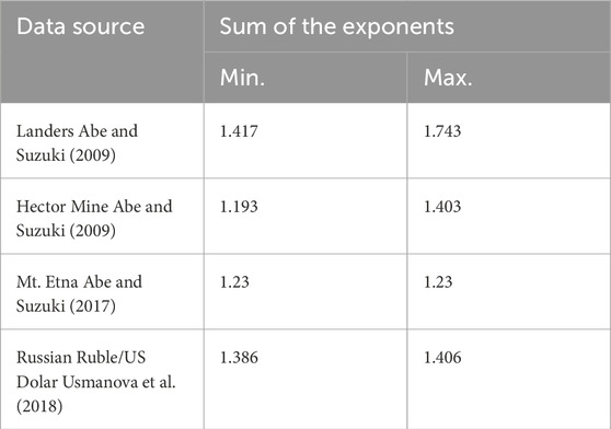
Table 1. Some reference examples in the literature.

The question of whether financial crisis processes that occur in a certain period after a crash are Markovian is intriguing. In Markovian processes, memory is short and fluctuations are localized. However, in non-Markovian processes, long-term memory and non-local fluctuations are observed, reflecting the complexity of the system. Studies have shown that volatility—specifically, the absolute value of returns—has long-term memory [20, 21]. Volatility values above a certain threshold will be referred to as events. These events correspond to shocks from an earthquake perspective.

In this study, we aim to examine whether the crisis process (bearish period) of Bitcoin (BTC) and Ethereum (ETH) after their peaks in 2017 (BTC), 2018 (ETH), and 2021 (BTC and ETH) is Markovian. At this point, the question of why cryptocurrencies may come to mind. The most important reason is that, unlike a traditional local stock exchanges, cryptocurrencies are traded globally and around the clock. The second factor is that this market is not regulated. Therefore, a piece of news (perhaps fake news) that hits the market at a time when the traditional stock market is closed may have an immediate impact on cryptocurrencies. However, as the day progresses, new information may emerge that calms the market and the news may even become irrelevant or vice versa. Therefore, over a long time horizon, fewer events may be observed compared to traditional markets. On the contrary, a cumulative effect in the opening minutes of the traditional market may manifest itself as a larger event than it should be. In addition, assuming that a large portion of cryptocurrency investors are less familiar with stock market dynamics, they might be more prone to emotional decision-making. Moreover, some dynamics may be easier to observe due to the higher volatility of cryptocurrencies compared to traditional markets.

2 Data set

To understand the dynamics of the market crash in cryptocurrencies, we analyzed the price movements of both BTC and ETH over six different periods. The data consists of minute-level candles, obtained from the Binance global exchange using its application programming interface (API). The aftershock regime in an earthquake is usually defined as the period following a mainshock, characterized by a large number of aftershocks. However, the Omori-Utsu Law does not dictate that the aftershock must be smaller than the mainshock, which is an important perspective. In financial markets, a crisis may begin with an initial downturn, subsequent downturns can be even more severe. Therefore, taking this into consideration and the classical approach of aftershock dynamics into account, three different time periods for both 2017 and 2021 cycles were prepared for the analysis. The first approach assumes that the crisis ends when the price returns to the same level. Second, we consider a scenario in which the crisis lasts from the price peak to the subsequent trough. Finally, we consider an interval after a large volatility. In this case, for 2017–2021 period, we consider the following for BTC: 1) A full cycle starting at its highest value (19,770.74 United States Dollar (USD)) on 17/12/2017 at 12:03 until 30/11/2020 at 23:52, when it returned to the same value. The interval contains 1,547,686 data points. 2) Again, the data interval starting on 17/12/2017 at 12:03 and ending at the trough (3157.67 USD) on 15/12/2018 at 15:51, which contains 518,896 data points. 3) Finally, we analyzed the time interval of 86,400 steps (60 days) after the largest volatility peak in the early days of the COVID-19 pandemic, which occurred on 12/03/2020 at 10:46. Similar intervals for ETH are as follows: 1) A cycle from 10/01/2018 at 04:58 (1433 USD) to 25/01/2021 at 00:23. This interval consists of 1,592,697 data points. 2) The interval from 10/01/2018 at 04:58 (1433 USD) to 15/12/2018 at 15:51 (82.03 USD) with 484,963 data points. 3) A time interval of 86,400 steps (60 days) after the largest peak in the early days of the COVID-19 pandemic, which occurred on 12/03/2020 at 23:28. The data sets for the 2021–2024 cycle for BTC are as follows: 4) A full cycle starting from its highest value (69,000 USD) on 10/11/2021 at 14:16 and ending when it reached the same value again on 08/03/2024 at 20:01. This cycle contains 1,222,826 data points. 5) The data set between the highest value on 10/11/2021 at 14:16 and the lowest value on 21/11/2022 at 21:51 (15,513 USD) contains 541,895 data points. 6) The last data set for Bitcoin includes 86,400 data points (60 days), starting from the highest volatility peak during the FTX crisis on 08/11/2022 at 19:34. 4) For ETH, there is no full cycle dataset after 2021 as it has not yet reached its all-time high (ATH) value. 5) The ATH for ETH is 4865 USD on 10/11/2021 at 14:16 and the lowest value after the ATH is 886 USD on 18/06/2022 at 20:11. The data set between these two points contains 317,157 data points. 6) The last dataset starts with the peak of volatility during FTX crisis on 10/11/2022 at 13:29 and includes 86,400 closing candles. These time intervals are summarized in Table 2.

Table 2

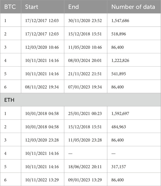
Table 2. The time intervals and the amount of data for each data set.

3 Methods

The scaling relation for singular Markov processes [16, 17] considers two key quantities for a point process. The first one is the distribution of the number of events in a time interval $\mathrm{\Delta }t$. This quantity corresponds to the Omori law for earthquakes and is given by

$n\left(t\right)=k{t}^{-p}(1)$

In Equation 1 $k$ is a positive constant and $p$ is an empirical exponent that characterizes the rate at which the number of events decreases with time. For earthquakes, this exponent usually takes values between 0.5 and 1.5. To obtain exponents more clearly, the cumulative number of events $N(t)$ will be used, as previously used in the analysis of stock market crashes in indices such as the Standard & Poor’s 500 Index (SP500), the National Association of Securities Dealers Automated Quotations (NASDAQ), and The New York Stock Exchange (NYSE) [9–11]. $N(t)$ is given as:

$N\left(t\right)=\frac{k}{1-p}{t}^{1-p}.(2)$

The use of the cumulative form of Omori law will be discussed again in Section 4. The behavior for the aforementioned scaling relation can be given asymptotically as follows:

$N\left(t\right)\sim t^{1-p}t\to \infty .(3)$

The second quantity is the waiting-time (i.e., interoccurrence time or calm-time) distribution, which is the distribution of time differences between successive events. This distribution is also in the form of a power law and can be given as

$P\left(\tau \right)\sim \frac{1}{{\tau }^{1+\mu }}\tau \to \infty .(4)$

If the process is Markovian, the relationship between the distribution of the number of events and the distribution of time intervals between successive events can be expressed as shown by Bardou et al. [16] and Barndorff-Nielsen et al. [17]

$S\left(t\right)=P\left(t\right)+{\int }_0^{t}d{t}^{\prime }P\left(t-t^{\prime }\right)S\left(t^{\prime }\right)(5)$

where $S(t)$ can be expressed in relation to the Omori law, as described by Abe and Suzuki [15],

$S\left(t\right)=\frac{dN\left(t\right)}{dt}=t^{-p}t\to \infty .(6)$

The Laplace transform of the Equation 5 is given as

$\mathcal{L}\left[S\right]\left(s\right)=\frac{\mathcal{L}\left[P\right]\left(s\right)}{1-\mathcal{L}\left[P\right]\left(s\right)}.(7)$

The relationship between the two exponents can be established by employing the Laplace transforms of Equation 4 and Equation 6 within the context of Equation 7. It is only valid in the range $0<p<1$ and $0<\mu <1$, and if the process is a singular Markov process, the relationship can be given as:

$p+\mu =1.(8)$

As can be seen from Equation 8, the scaling method has the advantage of being easy to apply. However, the method is limited by its sensitivity to the number of data and the requirement that the exponents lie within the range (0,1).

4 Results

To analyze whether the crisis process for BTC and ETH is Markovian, both the Omori law and the waiting-time distribution are studied over different time intervals. For BTC and ETH, a total of 11 different time intervals are defined, and therefore 11 different data sets are created and analyzed. These datasets consist of 1-min candle closing prices (X(t)), as mentioned in Section 2, and the return is given as:

$R\left(t\right)=\frac{X\left(t+1\right)-X\left(t\right)}{X\left(t\right)}.(9)$

The absolute value of the return (Equation 9) serves as a measure of volatility. The standard deviations for each data set are calculated separately to detect events. In this study, volatility and threshold values $q$ are presented in tables, expressed in units of standard deviation $\sigma$. The 1-minute return and volatility of BTC in data set 1 are shown in Figure 1. Volatility above a certain threshold is considered an event, and these time steps are recorded. Using this data, the distribution of the total number of events exceeding a certain threshold is calculated. Figure 2a shows the distribution of the total number of volatility events $N(t)$ exceeding the $3\sigma$ threshold for data set 1 of BTC. In the figure, the blue dots represent $N(t)$, while the red line represents the best fit to Equation 2.

Figure 1

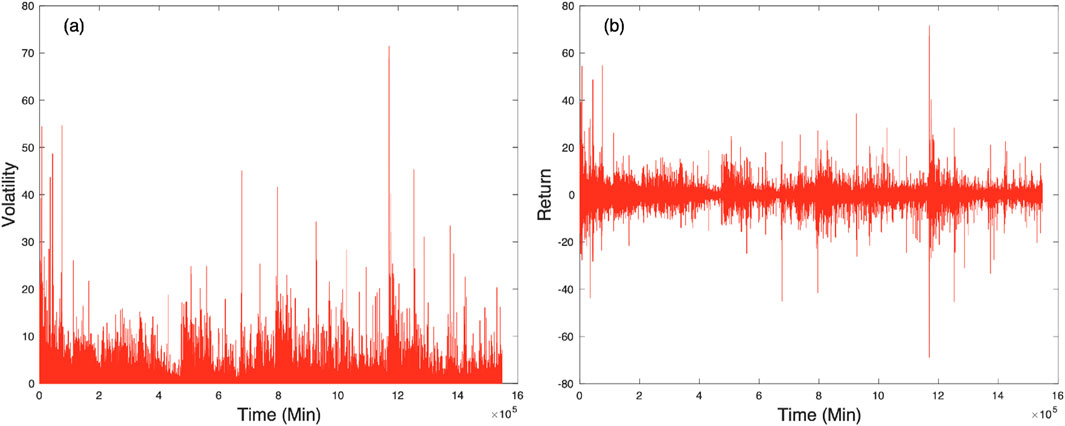
Figure 1. One-minute volatility (a) and return (b) of BTC over an approximately 3-year period after the 2017 all-time high (17 December 2017). Both return and volatility are measured in units of standard deviation $\sigma$, computed over the entire period.

Figure 2

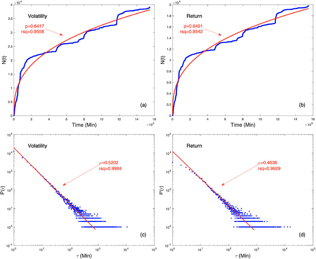
Figure 2. The cumulative number of events $N(t)$ for volatility (a) larger than a threshold $q=3\sigma$ and return (b) less than a threshold $q=-3\sigma$ are shown. Blue dots represent the cumulative number of events $N(t)$ and the red line represents the power-law fit to the data. The waiting-time distribution of volatility (c) and return (d) are also displayed. Blue dots represent the waiting-time distribution and the red line represents the power-law fit to the data. Also, rsq represents $r^2$ statistics for each fit.

The existence of the Omori regime in financial crises was first demonstrated by Lillo and Mantegna [9]. Weber et al. concluded that volatility has a memory, which is related to the Omori regime. It has also been shown that after events (aftershocks) following a main event (main shock) have their own Omori regime [11]. In these studies, volatility values were analyzed for a short time interval of 2 months. It would be insightful to examine the results for longer time intervals. On the other hand, since crashes are of primary interest, using returns below a certain value can also be a reasonable option. For the return threshold, we again use negative integer multiples of the standard deviation of the volatility data set. As expected, the number of events with unchanged behavior is halved for returns. It can be concluded that the minute price movements during the crash are not characterized by sharp falls and gradual rises, but rather by rises that are similar in character to the falls. As shown in Tables 3, 4, the Omori law is satisfied not only for a certain time interval after the highest volatility value, but also for almost the 3-year cycle. At this point, let us return to why we use a cumulative distribution as in Figure 3a. When a non-cumulative distribution is applied to financial data and a log–log plot is plotted, as shown in Figure 3b, a power-law-like behavior is observed in a very short interval. However, the possible Omori regime quickly disappears or seems to be masked by background fluctuations. A similar phenomenon can be observed in earthquakes. In general, faults within continents are reloaded slower than those at plate boundaries. On such slow-loading faults, the number of aftershocks after the main shock can decrease rapidly, and background seismicity becomes dominant. However, on such faults, aftershocks can persist for more than a century [22]. From a similar perspective, financial markets can also experience sudden shocks, and it can take many years to recover from a crisis situation. However, there are investors who trade short-term trends, regardless of whether the market is bullish or bearish. Perhaps, a significant amount of trading is done by bots. The orders placed by these accounts can trigger each other in the market, creating mini-crashes or spikes. These mini-crashes can create a background effect, masking a prolonged aftershock regime. Therefore, one can check whether the crisis process is Markovian in order to see whether there are background fluctuations in addition to crashes. As mentioned earlier, Markovian processes are characterized by local fluctuations and short-term memory. Assuming that background events are more localized, the fact that the process is Markovian means that background events dominate. On the contrary, the existence of events with long-term interactions implies that the process is non-Markovian. Therefore, the sum in Equation 8 is expected to deviate from 1 in the second scenario.

Table 3

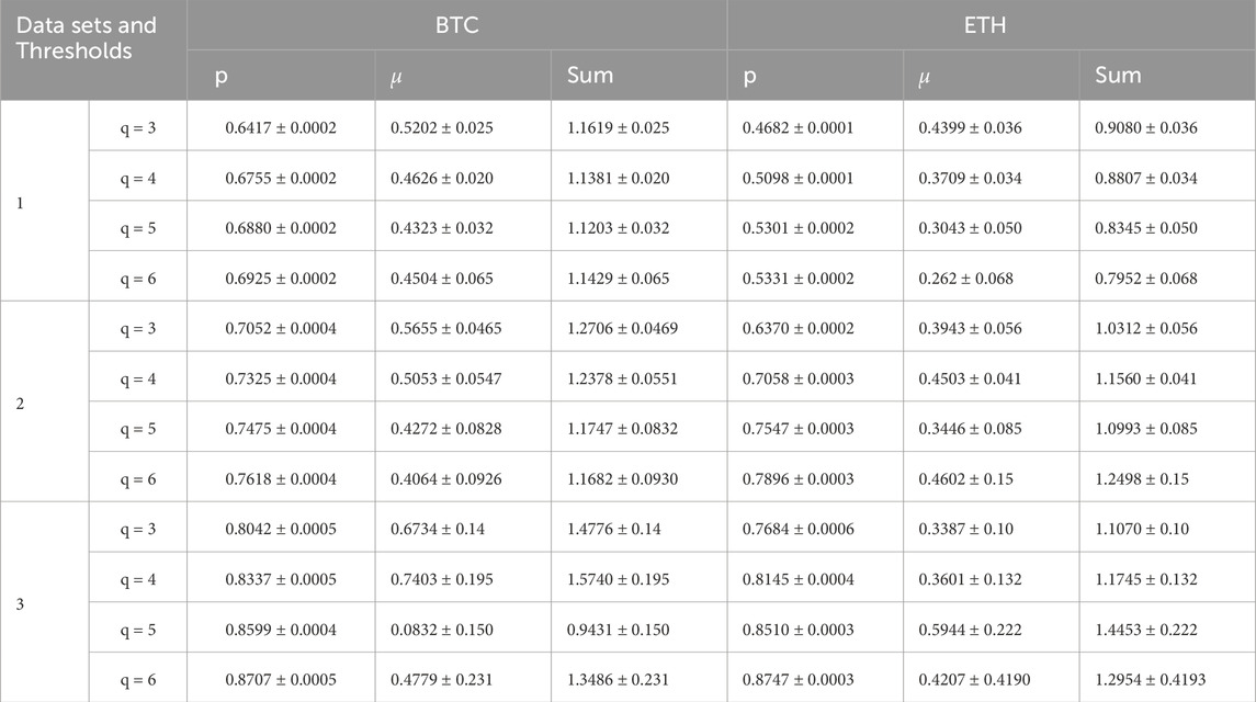
Table 3. The values of the exponents $p$ and $\mu$ for both BTC and ETH from 2017 to 2021.

Table 4

Table 4. The values of the exponents $p$ and $\mu$ for both BTC and ETH from 2021 to 2024.

Figure 3

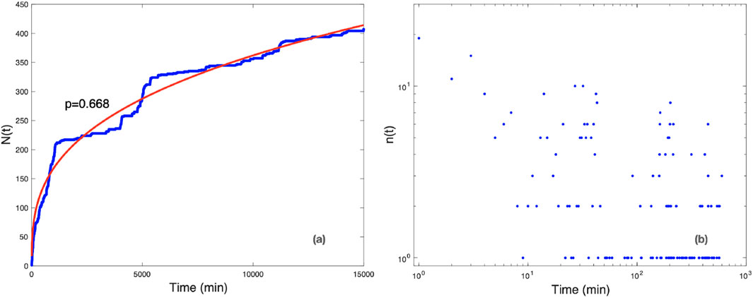
Figure 3. Comparison between the cumulative number of events $N(t)$ (a) and the log–log plots of the number of events (box sizes are 240 min) (b) after the $70\sigma$ volatility event in March 2020. The length of the data is 16,000 min.

Figure 2c shows the distribution of the waiting time between two successive BTC events. The distribution is in power-law form, and logarithmic binning was applied when calculating the exponent [23]. In Figures 2b,d, the same graphs are shown for return. As can be seen, the number of events has been approximately reduced by half, but the behavior has not changed. In Figure 2d, the decrease in the number of events appears as downward deviations from the fit curve at small $\tau$ values (a few points at the beginning) and more distortion at large $\tau$ values compared to the volatility graph. Although slight distortions were observed in all return examinations, we did not include the return values in the tables since the overall behavior remained unchanged. However, to illustrate the return behavior, we included it in Figure 2. Table 3 shows the $p$ and $\mu$ exponents given in Equation 3 and Equation 4, along with the sums of these two exponents for the 2017–2021 period.

For the first two data sets in BTC, the Omori regime exponent $p$ increases gradually as the threshold increases, indicating that larger events in the system end earlier and the system settles quickly. On the contrary, $\mu$ decreases with increasing threshold, indicating that the probability of observing longer waiting times between two events increases. The sum of these two exponents indicates that the process exhibits a non-Markovian character. However, as the threshold increases, this sum approaches slightly closer to 1.

The Omori regime exponent $p$ increases with the threshold as expected for ETH. Similar to BTC, the system settles down faster due to the smaller number of large events. In the ETH data set 1, which spans for a period of approximately 3 years, $\mu$ decreases, while for the shorter interval (about 1 year) it fluctuates. Considering the sum of these values, the first volatility data set shows a negative deviation from 1, while the second data set shows a positive deviation.

Since previous studies [9–11, 19] that show the existence of Omori regime behavior in financial markets focused on relatively short time intervals, we considered a similar length of time. We examined a dataset of 86,400 min (60 days) following the initial days of high volatility triggered by the COVID-19 pandemic to ensure similarity with previous studies. Despite many instances of high volatility in the 3-year period following the ATH, we observed that in some cases, without significant news affecting the market, the frequency of events was monotonous, and the analysis did not work for certain portions of such datasets. Therefore, we focused on a crisis following an event that profoundly impacted all markets, such as the COVID-19 pandemic. Compared to the other two datasets, the number of events in this 2-month data set decreased sharply. This reduction leads to greater dispersion in the tail of the waiting-time distribution and increased fluctuations in the slope $\mu$. Nevertheless, the total value tends to remain above 1, indicating non-Markovian behavior.

We also analyzed the period between 2021 and 2024. The number of events did not increase sharply after ATH for data 4 (graphs for all data sets are provided in the supplementary file). However, in the other datasets, events tend to occur more frequently after the onset of the bearish season. This almost monotonic event frequency in data 4 not only lowers the $p$ slope but also reduces the $\mu$ value, as it suppresses the occurrence of consecutive events within short intervals. Consequently, unlike the previous cycle, BTC’s second full cycle, which began in 2021, deviates negatively from 1. This pattern is similar to the first full cycle of ETH. Additionally, since ETH has not yet reached its ATH again, a full cycle period could not be studied for ETH and is therefore not included in Table 4.

For the ATH to all-time low (ATL) values, data were examined within the intervals mentioned in Section 2. It was observed that events occurred relatively more frequently in the last quarter of the data. This dominance significantly affects the value of the $p$ slope. For both BTC and ETH, $p<0$ was observed for all $q$ values. Therefore, the analysis does not work for these data sets, and no values are provided in Table 4 for dataset 5.

For the last dataset, a disruptive event in the cryptocurrency markets—the collapse of the FTX exchange—was chosen, and the period following this event was examined. After news emerged regarding FTX’s cash problems on 2 November 2022, a sharp withdrawal that shook the cryptocurrency market occurred between November 6 and November10. When examining the dataset of 86,400 steps after the highest volatility value during this collapse, the $p$ and $\mu$ values for BTC show a similar pattern to those observed during the COVID-19 period. The total also shows a deviation greater than 1. Therefore, non-Markovian behavior is more pronounced during this period. In the analysis of ETH during the same time frame, it was observed that the $\mu$ value exhibits high volatility and significant error margins. Although there is a tendency for the total to be greater than 1 for most $q$ values, the high error margins prevent any conclusions from being drawn regarding non-Markovian behavior.

We also repeated the analysis for closing candles of different lengths, such as 5 min, 15 min, 1 h, and 1 day. As expected, the fluctuations in the waiting-time distribution increase as the amount of data decreases, significantly affecting the margin of error in the slope of the waiting-time distribution. Even with increasing $q$ values, the margins of error become larger than the slope itself. Again, as the value of $q$ increases, it was observed that $\mu$ falls outside its definition range. For this reason, data from other candle closings are not included in the tables. However, we observed that the sum deviates negatively from 1 when the $p$ and $\mu$ values remain within their defined range for certain $q$ values.

At this point, one might wonder whether traditional stock markets exhibit similar behavior. The analysis was repeated for the Istanbul Exchange 100 Index (BIST-100) during the crash period in 2008. However, it is not possible to draw any conclusions about Markovianity for short time intervals because of very large fluctuations in the waiting-time distribution. However, unlike BTC and ETH, the Omori regime was not observed for the long time interval. For this reason, the BIST-100 analysis and graphs are not provided.

5 Conclusion

The statistical characteristics of the bearish season in cryptocurrencies were analyzed. It is shown that the scaling relation, which is valid for a singular Markovian process, is violated. This violation serves as evidence of the non-Markovian nature of the crises process. This result is very important from a financial market perspective, as it is indicates long-range memory and non-local fluctuations. These effects may arise as a reflection of wild volatility in cryptocurrencies. It should also be noted that this market is not regulated. As the scaling method is not applicable to the BIST100 index, the results could not be compared to a regulated market. Both the lack of comparability and the sensitivity to data size imply that further studies are needed.

It is also shown that the distribution of the cumulative number of volatilities and return events for BTH and ETH is consistent with Equation 2 for both short and long time intervals. In the literature, based on the existence of the Omori law, it has been shown that such fluctuations exhibit memory for short time intervals in stock markets such as the S&P 500 and Nasdaq [10, 11]. Our analyses show that both the COVID-19 pandemic and the FTX crisis yield results consistent with these previous findings. These analyses demonstrate that the behavior of both BTC and ETH is non-Markovian, indicating that their volatility exhibits a memory effect.

Data availability statement

Publicly available datasets were analyzed in this study. These data can be found here: The relevant data were downloaded from the Binance Global exchange using the API.

Author contributions

AC: conceptualization, data curation, formal analysis, investigation, methodology, project administration, resources, software, supervision, validation, visualization, writing – original draft, and writing – review and editing.

Funding

The author(s) declare that no financial support was received for the research and/or publication of this article.

Conflict of interest

The author declares that the research was conducted in the absence of any commercial or financial relationships that could be construed as a potential conflict of interest.

Generative AI statement

The author(s) declare that no Generative AI was used in the creation of this manuscript.

Publisher’s note

All claims expressed in this article are solely those of the authors and do not necessarily represent those of their affiliated organizations, or those of the publisher, the editors and the reviewers. Any product that may be evaluated in this article, or claim that may be made by its manufacturer, is not guaranteed or endorsed by the publisher.

References

1. Jay P, Kalariya V, Parmar P, Tanwar S, Kumar N, Alazab M. Stochastic neural networks for cryptocurrency price prediction. IEEE Access (2020) 8:82804–18. doi:10.1109/ACCESS.2020.2990659

CrossRef Full Text | Google Scholar

2. Jagannath N, Barbulescu T, Sallam KM, Elgendi I, Okon AA, Mcgrath B, et al. A self-adaptive deep learning-based algorithm for predictive analysis of bitcoin price. IEEE Access (2021) 9:34054–66. doi:10.1109/ACCESS.2021.3061002

CrossRef Full Text | Google Scholar

3. Erfanian S, Zhou Y, Razzaq A, Abbas A, Safeer AA, Li T. Predicting bitcoin (btc) price in the context of economic theories: a machine learning approach. Entropy (2022) 24:1487. doi:10.3390/e24101487

PubMed Abstract | CrossRef Full Text | Google Scholar

4. Scagliarini T, Pappalardo G, Biondo AE, Pluchino A, Rapisarda A, Stramaglia S. Pairwise and high-order dependencies in the cryptocurrency trading network. Scientific Rep (2022) 12:18483. doi:10.1038/s41598-022-21192-6

PubMed Abstract | CrossRef Full Text | Google Scholar

5. Gutenberg B, Richter CF. Frequency of earthquakes in California. Bull Seismilogical Soc Am (1944) 34:185–8. doi:10.1785/bssa0340040185

CrossRef Full Text | Google Scholar

6. Omori F. On the after-shocks of earthquakes. J Coll Sci (1894) 7:111–200.

Google Scholar

7. Utsu T. A statistical study on the occurrence of aftershocks. Geophys Mag (1961) 30:521–605.

Google Scholar

8. Båth M. Lateral inhomogeneities of the upper mantle. Tectonophysics (1965) 2:483–514. doi:10.1016/0040-1951(65)90003-x

CrossRef Full Text | Google Scholar

9. Lillo F, Mantegna RN. Power-law relaxation in a complex system: omori law after a financial market crash. Phys Rev E (2003) 68:016119. doi:10.1103/PhysRevE.68.016119

PubMed Abstract | CrossRef Full Text | Google Scholar

10. Petersen AM, Wang F, Havlin S, Stanley HE. Market dynamics immediately before and after financial shocks: quantifying the omori, productivity, and bath laws. Phys Rev E (2010) 82:036114. doi:10.1103/PhysRevE.82.036114

PubMed Abstract | CrossRef Full Text | Google Scholar

11. Weber P, Wang F, Vodenska-Chitkushev I, Havlin S, Stanley HE. Relation between volatility correlations in financial markets and omori processes occurring on all scales. Phys Rev E (2007) 76:016109. doi:10.1103/PhysRevE.76.016109

PubMed Abstract | CrossRef Full Text | Google Scholar

12. Da Cunha C, Da Silva R. Relevant stylized facts about bitcoin: fluctuations, first return probability, and natural phenomena. Physica A (2020) 550:124155. doi:10.1016/j.physa.2020.124155

CrossRef Full Text | Google Scholar

13. Selçuk F, Gençay R. Intraday dynamics of stock market returns and volatility. Physica A (2006) 367:375–87. doi:10.1016/j.physa.2005.12.019

CrossRef Full Text | Google Scholar

14. Siokis FM. Stock market dynamics: before and after stock market crashes. Physica A (2012) 391:1315–22. doi:10.1016/j.physa.2011.08.068

CrossRef Full Text | Google Scholar

15. Abe S, Suzuki N. Violation of the scaling relation and non-markovian nature of earthquake aftershocks. Physica A (2009) 388:1917–20. doi:10.1016/j.physa.2009.01.031

CrossRef Full Text | Google Scholar

16. Bardou F, Bouchaud J-P, Aspect A, Cohen-Tannoudji C. Lévy statistics and laser cooling: how rare events bring atoms to rest. Cambridge University Press (2002).

CrossRef Full Text | Google Scholar

17. Barndorff-Nielsen OE, Benth FE, Jensen JL. Markov jump processes with a singularity. Adv Appl Probab (2000) 32:779–99. doi:10.1239/aap/1013540244

CrossRef Full Text | Google Scholar

18. Abe S, Suzuki N. Subdiffusion of volcanic earthquakes. Acta Geophys (2017) 65:481–9. doi:10.1007/s11600-017-0029-6

CrossRef Full Text | Google Scholar

19. Usmanova V, Lysogorskiy YV, Abe S. Aftershocks following crash of currency exchange rate: the case of rub/usd in 2014. EPL (2018) 121:48001. doi:10.1209/0295-5075/121/48001

CrossRef Full Text | Google Scholar

20. Cizeau P, Liu Y, Meyer M, Peng C-K, Stanley HE. Volatility distribution in the s&p500 stock index. Physica A (1997) 245:441–5. doi:10.1016/S0378-4371(97)00417-2

CrossRef Full Text | Google Scholar

21. Liu Y, Gopikrishnan P, Stanley HE, Meyer , Peng . Statistical properties of the volatility of price fluctuations. Phys Rev E (1999) 60:1390–400. doi:10.1103/physreve.60.1390

CrossRef Full Text | Google Scholar

22. Stein S, Liu M. Long aftershock sequences within continents and implications for earthquake hazard assessment. Nature (2009) 462:87–9. doi:10.1038/nature08502

PubMed Abstract | CrossRef Full Text | Google Scholar

23. Christensen K, Moloney NR. Complexity and criticality, 1. World Scientific Publishing Company (2005).

Google Scholar