Modeling and numerical analysis for an MEMS graphene resonator

This paper delves into the static and dynamic behavior of graphene cantilever beam resonators under electrostatic actuation at their free tips. A rigorous analysis of the system’s response is performed. The constitutive nonlinear equation of the system is derived using the energy method and Hamilton’s principle. An analytical solution to the nonlinear static problem is obtained. The generalized stiffness coefficient for the lumped model of the cantilever graphene beam under load at its tip is calculated, enabling a comprehensive analysis of its dynamic behavior. A key focus is on investigating the dynamic pull-in conditions of the system under both constant and harmonic excitation. Analytical predictions are validated through numerical simulations. The system exhibits periodic solutions when the excitation parameters are below a certain threshold described by a separatrix curve, leading to sustained oscillations. On the other hand, if the excitation parameters exceed this threshold, the system experiences pull-in instability, causing the beam to touch down. Furthermore, we explore the impact of excitation frequency on the dynamic response of the graphene cantilever beam under harmonic load. The simulations reveal that choosing the excitation frequency near the beam’s resonance frequency can lead to structural collapse under certain parameter conditions.

1 Introduction

Microelectromechanical systems (MEMS) have revolutionized numerous fields by enabling the creation of miniaturized devices with remarkable performance and functionalities. MEMS devices are distinguished by their compact size, low power consumption, and ability to integrate mechanical, electrical, and optical features on a single chip [1]. Among the vital components of MEMS are microresonators that are excited near their resonance frequencies. These microresonators find extensive applications in mass and force sensors, including the detection of proteins [2], molecules [3], electrons, and nanoparticles [4]. However, the sensitivity of these sensors can be improved by addressing the weight of the microbeam, as the minimum detectable quantity is often limited by the mass of the resonator. Therefore, lightweight and high-strength materials are highly desirable to overcome this limitation.

In this context, graphene has emerged as a promising material for MEMS and microresonators due to its light weight and outstanding mechanical properties, including high Young’s modulus and tensile strength. Table 1 shows the summary of graphene’s mechanical characteristics compared to common MEMS components such as steel and silicon.

Table 1

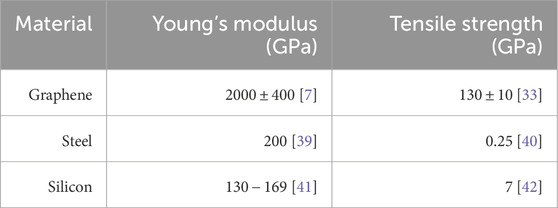
Table 1. Mechanical properties of graphene, steel, and silicon.

Graphene is a single layer of carbon atoms tightly bound together. The superior properties of graphene stem from its carbon-carbon bond structure and ${\text{sp}}^2$ hybridization [5]. Beyond its exceptional mechanical properties, graphene also exhibits remarkable electronic characteristics, making it a prime candidate for spintronics and pseudospintronics applications in Pesin and MacDonald [6]. This unique arrangement gives graphene remarkable mechanical properties, including a high Young’s modulus of 2 TPa [7] and a failure strength that is significantly greater than that of the strongest steel [8]. It also grants it remarkable ductility, making it stretchable by up to 20$\%$ [9]. Its possible uses span several areas, such as the creation of transparent electrodes, ultra-strong composites, and flexible, stretchable screens for display or energy storage purposes [10]. Additionally, graphene’s topological properties have been explored in the context of bound states and conical singularities, which could further enhance its functionality in next-generation nanodevices, as in Rüegg and Lin [11].

Interestingly, though graphene was not originally thought to exhibit piezoelectric properties due to its symmetry, recent advancements have enabled its application in the field of micro and nano-electromechanical systems (MEMS/NEMS). This could enable the development of new energy harvesting, actuation, and transduction technologies [12]. Furthermore, graphene’s high sensitivity and low mass make it an ideal candidate for high-resolution mass sensing, and its high thermal conductivity suggests potential use as a thermal management material [13]. Its thermal conductivity at room temperature equals $500W{m}^{-1}{K}^{-1}$ [14]. It is worth mentioning the importance of graphene’s adhesion energy with substrates for the stable, long-term operation of micro and nanodevices. Furthermore, the exceptional tribological properties of graphene make it beneficial for reducing friction and offering protection against corrosion [10, 15].

Graphene’s remarkable attributes offer opportunities for further miniaturization of MEMS resonators and have led to a new wave of research in this area. Utilizing graphene resonators in mass detection has become a particularly compelling topic of study. For example, in [16], it was found that nonlinear vibrations can enhance the sensitivity of a graphene microbeam resonator. A related approach involves studying nonlinear solutions, which have been widely applied in mathematical models of wave propagation and stability analysis in nonlinear systems in Li and Yu [17]. Natsuki et al., employing the continuum elasticity theory, have shown that the mass sensors with double-layered graphene sheets (DLGSs) provide higher sensitivity than single-layered graphene sheets (SLGSs) [18]. Another way to increase the detection sensitivity has been studied by Karličić et al. [19]. The study associates it with the increase in the magnetic field that results in the sensor’s frequency shift. Many works study the potential applications of graphene microresonators through experimental results. However, we are interested in the mathematical analysis of such systems. For instance, Wei et al. investigated the steady-state behavior of a graphene Euler beam subjected to a constant load and provided analytical and finite element solutions [20]. Using the Rayleigh–Ritz method with Hermite cubic interpolation yielded approximate finite element solutions, which were validated against analytical solutions.

Several studies have investigated the dynamic behavior of electrostatically actuated systems made of graphene. Among the notable research works are Anjum and He [21], Kadyrov et al. [22], Skrzypacz et al. [23], Wei et al. [24], and Omarov et al. [25]. Recent studies on soliton dynamics in nonlinear Schrödinger-type equations in Qing et al. [26] provide insights into analytical approaches that could complement the study of nonlinear MEMS resonators. Electrostatic actuation is widely preferred in the field of microelectromechanical systems due to its simplicity and efficiency, offering advantages over alternative actuation methods such as electrothermal, piezoelectric, and electromagnetic actuation [1, 27]. When electrostatically actuated resonators are employed, the electric load applied to a cantilever beam comprises both AC and DC components. The DC component induces deflection of the beam to its equilibrium position, while the AC component generates vibrations around this equilibrium position. The equilibrium position is attained when the restoring force of the beam matches the electrostatic force [1].

However, if the DC polarization voltage is increased beyond a certain threshold, exceeding the restoring force, the beam continues to deflect until it contacts an adjacent structure or surface, resulting in collapse. This phenomenon is known as the pull-in instability, and the threshold voltage at which it occurs is referred to as the pull-in voltage. Pull-in can be classified into two types: static pull-in and dynamic pull-in. Static pull-in describes the occurrence of pull-in solely due to DC actuation, while dynamic pull-in can arise from AC harmonic excitation or the motion of the structure [1]. Analyzing and understanding pull-in is essential in the design of MEMS resonators. It is crucial to tune the electric load parameters to avoid pull-in instability, as it can lead to structural collapse and device failure. Skrzypacz et al. [23] conducted a comprehensive investigation, providing the necessary and sufficient conditions for the existence of periodic solutions for a lumped mass model subjected to a constant DC voltage. This study contributed valuable insights into the dynamic behavior of the model under a constant loading scenario. Additionally, the pull-in phenomenon of the same lumped mass model excited by a harmonic load was explored in two separate research works: Kadyrov et al. [22] and Omarov et al. [25]. In Omarov et al. [25], Sturm’s theorem was employed to identify periodic solutions of the lumped mass model with general initial conditions, and their analytical results were verified through numerical simulations implemented in the Python programming language. Furthermore, the work of Anjum and He [21] and Wei et al. [24] delved into the study of the nonlinear graphene beam equation and the existence of several natural frequencies of the system. These studies utilized the variational iteration method based on a Laplace transform and the Pade technique to obtain approximate solutions. Recent examples of approximation techniques for periodic solutions to MEMS oscillators can be found in He [28], while the pull-down instability of the nonlinear quadratic oscillators is investigated in He et al. [29]. Studies on nonlinear wave equations have shown that higher-order dispersion effects play a crucial role in the stability and response of nonlinear systems, as in Li and Fajun [30].

This paper investigates the static and dynamic behavior of a graphene cantilever beam subjected to electrostatic actuation at its free tip. The same oscillator model proposed in Skrzypacz et al. [31] is employed, comprising a low-mass graphene beam of length $\ell$, an inflexible platform acting as a movable electrode attached to the free end of the beam, and a fixed electrode covered with a dielectric layer of thickness $h$ and dielectric constant ${\epsilon }_r$, as shown in Figure 1. The potential difference and gap between the two electrodes are represented by $V$ and $d$, respectively. The interaction of attractive electrostatic force due to the potential difference and the nonlinear restoring force of the beam is expected to lead to high-frequency oscillations. The role of nonlocal interactions in phononic lattices, which share similarities with graphene-based resonators, has also been studied to understand their impact on bound modes and wave propagation in Poggetto et al. [32].

Figure 1

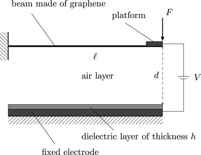
Figure 1. A schematic of a graphene microresonator.

The study is structured as follows: In Section 2, the constitutive nonlinear equation governing the system is derived using the energy method and Hamilton’s principle, and boundary conditions are established. In Section 3, an analytical solution for the static problem is computed. Section 4 presents the development of a lumped mass model, which is employed to study the fundamental dynamics of the system and also provides the calculation of the generalized stiffness coefficient for the graphene cantilever beam under the load at its tip. The pull-in phenomenon under both constant and harmonic excitation is analyzed in Section 5. Simulation results for dynamic pull-in and resonance are presented in Section 6. Finally, conclusions are drawn in Section 7.

2 Mathematical model

This section focuses on deriving the constitutive nonlinear equation for a cantilever beam made of graphene by employing Hamilton’s principle, an essential concept in variational mechanics.

2.1 Constitutive stress–strain equation for graphene

It is theoretically and experimentally justified that the stress–strain relationship for the classical Euler–Bernoulli beam made of graphene can be written as

$\sigma =E\epsilon +D|\epsilon |\epsilon ,(1)$

where $\sigma$, $\epsilon$, and $E$ are the stress, strain, and Young’s modulus and $D=-E^2/4{\sigma }_{\mathit{max}}$ is the second-order elastic stiffness constant [33, 34]. The negative value of $D$ is associated with reduced stiffness at high tensile strains and increased stiffness at high compressive strains. The values of $E$ and $D$ were determined by Khan et al. [35] through the measurement of deformation in single-atomic-layer graphene sheets using nanoindentation with an atomic force microscope. The experimental findings yielded a value of $E$ as $2.4\pm 0.04\text{\hspace{0.17em}TPa}$ and $D$ as $-2.0\pm 0.4\text{\hspace{0.17em}TPa}$. According to Lee et al. [33], the nonlinearity of the stress–strain response of graphene arises from the third-order term of a strain-dependent energy potential expressed as a Taylor series. This characterization of the stress–strain behavior of graphene will be utilized in the forthcoming modeling section.

2.2 Model equation for a Euler–Bernoulli beam made of graphene

Here, we consider a cantilever beam subjected to a force applied at the free end and analyze a small segment on the beam before and after deflection (see Figure 2). In the following, $w=w(t,x)$ denotes the deflection of the beam at time $t$ and axial position $x$. According to the Euler–Bernoulli beam theory, the cross section of the beam remains plane and perpendicular to the beam’s centerline [1]. To analyze the behavior of the beam, it is necessary to determine the axial strain at a specific point, denoted as point $B$, located at a distance $y$ from the centerline; see Figure 2. In the given figure, the axial displacement of point $B$ caused by pure bending is represented as $u_b$, and it is expressed as

$u_b=-y{w}^{\prime }.$

Figure 2

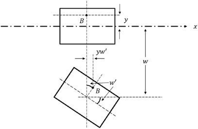
Figure 2. A segment of a beam before and after bending.

The axial strain ${\epsilon }_b$ can be calculated as

${\epsilon }_b=\frac{\partial u_b}{\partial x}=-y{w}^{″}.$

By integrating the stress–strain Equation 1 with respect to strain, we obtain the strain energy density, which represents the energy stored per unit volume in the material. This energy density is a measure of the potential energy stored within the beam due to deformation. Integrating this quantity over the entire volume of the beam allows us to determine the total potential energy of the system. Thus, we get

$U=\frac{1}{2}E\epsilon {\epsilon }^{\mathcal{T}}+\frac{1}{3}D|\epsilon |\epsilon {\epsilon }^{\tau },(2)$

where $U$ is the strain energy density, and $\epsilon =({\epsilon }_x,{\epsilon }_y,{\epsilon }_z,{\gamma }_{xy},{\gamma }_{xz},{\gamma }_{yz})$ is the strain, and where ${\epsilon }_x=\frac{\partial u}{\partial x}$, ${\epsilon }_y=\frac{\partial w}{\partial y}$, ${\epsilon }_z=\frac{\partial v}{\partial z}$, ${\gamma }_{xy}=\frac{1}{2}\left(\frac{\partial u}{\partial y}+\frac{\partial w}{\partial x}\right)$, ${\gamma }_{xz}=\frac{1}{2}\left(\frac{\partial u}{\partial z}+\frac{\partial v}{\partial x}\right)$, and ${\gamma }_{yz}=\frac{1}{2}\left(\frac{\partial w}{\partial z}+\frac{\partial v}{\partial y}\right)$ are the strain components. For the Euler–Bernoulli beam, it is assumed that

${\epsilon }_x=\frac{\partial u}{\partial x}=-y{w}^{″}={\epsilon }_b,$

and

${\epsilon }_y={\epsilon }_z={\gamma }_{xy}={\gamma }_{xz}={\gamma }_{yz}=0.$

Therefore, Equation 2 simplifies to

$U=\frac{1}{2}E{\epsilon }_x^2+\frac{1}{3}D|{\epsilon }_x|{\epsilon }_x^2.$

Then, the total potential energy $E_{\mathit{pot}}$ can be expressed as

$E_{\mathit{pot}}=\frac{1}{2}{\int }_{V}E{\epsilon }_x^{2}dV+\frac{1}{3}{\int }_{V}D|{\epsilon }_x|{\epsilon }_x^{2}dV.(3)$

Inserting the axial strain into Equation 3 yields

$\begin{array}{cc}\hfill E_{\mathit{pot}}& =\frac{1}{2}{\int }_{V}E{\left(-y{w}^{″}\right)}^{2}dV+\frac{1}{3}{\int }_{V}D|-y{w}^{″}|{\left(-y{w}^{″}\right)}^{2}dV\hfill \\ \hfill & =\underset{E_{\mathit{pot}}^{\left(1\right)}}{\underbrace{\frac{1}{2}{\int }_{V}E{\left(y{w}^{″}\right)}^{2}dV}}+\underset{E_{\mathit{pot}}^{\left(2\right)}}{\underbrace{\frac{1}{3}{\int }_{V}D|w^{″}|{\left(w^{″}\right)}^2{y}^{3}dV}}.\hfill \end{array}(4)$

Note that $y$ is the distance from the centerline. We have

$\begin{array}{cc}\hfill E_{\mathit{pot}}^{\left(1\right)}& =\frac{1}{2}{\int }_{V}E{\left(y{w}^{″}\right)}^{2}dV=\frac{1}{2}{\int }_0^{\ell }{\int }_{A}E{\left(y{w}^{″}\right)}^{2}dAdx\hfill \\ \hfill & =\frac{1}{2}{\int }_0^{\ell }E{\left(w^{″}\right)}^2\left({\int }_A{y}^{2}dA\right)dx,\hfill \end{array}(5)$

where $\ell$ is the length of the beam, and $A$ is the cross-sectional area. Expressing the second moment of inertia of the cross section as

$I_1={\int }_A{y}^{2}dA,$

Equation 5 can be rewritten as

$E_{\mathit{pot}}^{\left(1\right)}=\frac{E{I}_1}{2}{\int }_0^{\ell }{\left(w^{″}\right)}^{2}dx.(6)$

$E_{\mathit{pot}}^{(2)}$ is expanded in the similar manner:

$\begin{array}{cc}\hfill E_{\mathit{pot}}^{\left(2\right)}& =\frac{1}{3}{\int }_{V}D|w^{″}|{\left(w^{″}\right)}^2{y}^{3}dV=\frac{1}{3}{\int }_0^{\ell }{\int }_{A}D|w^{″}|{\left(w^{″}\right)}^2{y}^{3}dAdx\hfill \\ \hfill & =\frac{1}{3}{\int }_0^{\ell }D|w^{″}|{\left(w^{″}\right)}^2\left({\int }_A{y}^{3}dA\right)dx=\frac{D{I}_2}{3}{\int }_0^{\ell }|w^{″}|{\left(w^{″}\right)}^{2}dx,\hfill \end{array}(7)$

where

$I_2={\int }_A{y}^{3}dA$

is the third moment of inertia of the cross section. Inserting Equations 6, 7 into Equation 4 gives the following potential energy equation:

$E_{\mathit{pot}}=\frac{E{I}_1}{2}{\int }_0^{\ell }{\left(w^{″}\right)}^{2}dx+\frac{D{I}_2}{3}{\int }_0^{\ell }|w^{″}|{\left(w^{″}\right)}^{2}dx.$

The kinetic energy of a beam can be calculated based on the mass distribution along the length of the beam and the velocity of its individual mass elements. The general formula for the kinetic energy of a beam is given by

$E_{\mathit{kin}}=\frac{\rho A}{2}{\int }_0^{\ell }{\dot{w}}^{2}dx,$

where $\rho$ is material density, and $\dot{w}$ is the time derivative of the beam deflection $w(x,t)$. The work $W$ done by the external force on the cantilever beam at the free end can be written as

$W=Fw\left(\ell \right),$

where $w(\ell )$ is the deflection of the beam at $x=\ell$.

2.3 Hamilton’s principle

In order to derive the graphene beam equation of motion, we need to use the Lagrangian energy functional $I(w)$ and Hamilton’s principle [1, 36]. The Lagrangian energy functional is defined by

$\mathcal{I}\left(w\right)=E_{\mathit{kin}}\left(w\right)-E_{\mathit{pot}}\left(w\right)+W\left(w\right).$

Applying the Hamilton’s principle on the Lagrangian $I(w)$ gives

$\left.{\int }_{t_1}^{t_2}\delta \mathcal{I}\left(w\right)dt={\int }_{t_1}^{t_2}\left[\right]\delta E_{\mathit{kin}}\left(w\right)-\delta E_{\mathit{pot}}\left(w\right)+\delta W\left(w\right)\right]dt=0,(8)$

where $t_1$ and $t_2$ are two instants of time during which the system experiences the variation, and $\delta$ is the variation operator. The Hamilton’s principle requires calculating the variations of the work of the external force $(\delta W)$, the kinetic $\delta E_{\mathit{kin}}$ and potential $(\delta E_{\mathit{pot}})$ energies, simplifying and expressing in terms of variation displacement $\delta w$. The variation of the kinetic energy and the work is given as

$\delta W=F\delta w\left(\ell \right),$

and

$\delta E_{\mathit{kin}}=\rho A{\int }_0^l\dot{w}\delta \dot{w}dx.(12)$

By applying integration by parts to the variation of the kinetic energy expression by Equation 9, we can rewrite it in terms of the virtual displacement $\delta w$ as follows:

$\begin{array}{cc}\hfill {\int }_{t_1}^{t_2}\left(\delta E_{\mathit{kin}}\right)dt& ={\int }_{t_1}^{t_2}\left[\rho A{\int }_0^{\ell }\dot{w}\delta \dot{w}dx\right]dt=\rho A{\int }_0^{\ell }\left[{\int }_{t_1}^{t_2}\dot{w}\delta \dot{w}dt\right]dx\hfill \\ \hfill & =\rho A{\int }_0^{\ell }\left[\underset{=0}{\underbrace{{\left.\dot{w}\delta w\right|}_{t_1}^{t_2}}}-{\int }_{t_1}^{t_2}\ddot{w}\delta wdt\right]dx\hfill \\ \hfill & =\rho A{\int }_0^{\ell }\left[-{\int }_{t_1}^{t_2}\ddot{w}\delta wdt\right]dx.\hfill \end{array}(10)$

The boundary term in time vanishes in Equation 10 due to the boundary conditions imposed on the virtual displacement. Specifically, it is assumed that the virtual displacement satisfies $\delta w(t_1)=\delta w(t_2)=0$. The variation of the potential energy $E_{\mathit{pot}}$ can be written as

$\delta E_{\mathit{pot}}=E{I}_1{\int }_0^{\ell }{w}^{″}\delta w^{″}dx+D{I}_2{\int }_0^{\ell }|w^{″}|w^{″}\delta w^{″}dx.(11)$

To express Equation 11 in terms of displacement variation $\delta w$, several integrations by parts need to be implemented as shown below:

$E{I}_1{\int }_0^{\ell }{w}^{″}\delta w^{″}dx={\left.E{I}_1{w}^{″}\delta w^{\prime }\right|}_{s0}^{\ell }-{\left.E{I}_{1}w‴\delta w\right|}_0^{\ell }+E{I}_1{\int }_0^{\ell }{w}^{⁗}\delta wdx,(12)$

$\begin{array}{cc}\hfill D{I}_2{\int }_0^l|w^{″}|w^{″}\delta w^{″}dx={\left.D{I}_2|w^{″}|w^{″}\delta w^{\prime }\right|}_0^{\ell }\hfill & \hfill -D{I}_2{\left.{\left(|w^{″}|w^{″}\right)}^{\prime }\delta w\right|}_0^{\ell }\hfill \\ \hfill \hfill & \hfill +D{I}_2{\int }_0^{\ell }{\left(|w^{″}|w^{″}\right)}^{″}\delta wdx.\hfill \end{array}(13)$

Substituting Equations 12, 13 into Equation 8 and grouping the terms gives

$\begin{array}{cc}\hfill {\int }_{t_1}^{t_2}& \left\{{\int }_0^{\ell }\left[-\rho A\ddot{w}-E{I}_1{w}^{\prime \prime \prime \prime }-{DI}_2{\left(|w^{\prime \prime }|w^{\prime \prime }\right)}^{\prime \prime }\right]\delta wdx\right.\hfill \\ \hfill & -\left[E{I}_1{w}^{\prime \prime }+D{I}_2|w^{\prime \prime }|w^{\prime \prime }\right]\delta {\left.w^{\prime }\right|}_0^{\ell }\hfill \\ \hfill & +\left[E{I}_1{w}^{\prime \prime \prime }+D{I}_2{\left(|w^{\prime \prime }|w^{\prime \prime }\right)}^{\prime }+F\right]\delta w\left(\ell \right)\hfill \\ \hfill & \left.-\left[E{I}_1{w}^{\prime \prime \prime }+D{I}_2{\left(|w^{\prime \prime }|w^{\prime \prime }\right)}^{\prime }\right]\delta w\left(0\right)\right\}dt=0.\hfill \end{array}(14)$

According to the definition, the variation $\delta w$ and $\delta u$ are arbitrary; therefore, each group of terms must be 0 in order to satisfy Equation 14, which leads to the following equation of motion and boundary conditions:

$\rho A\ddot{w}+E{I}_1{w}^{⁗}+D{I}_2{\left(|w^{″}|w^{″}\right)}^{″}=0,$

$E{I}_{1}w‴+D{I}_2{\left(|w^{″}|w^{″}\right)}^{\prime }=0;\text{or}\delta w=0\text{at}x=0,$

$E{I}_{1}w‴+D{I}_2{\left(|w^{″}|w^{″}\right)}^{\prime }=-F;\text{or}\delta w=0\text{at}x=\ell ,(15)$

$E{I}_1{w}^{″}+D{I}_2|w^{″}|w^{″}=0;\text{or}\delta w^{\prime }=0\text{at}x=0,\ell .(16)$

Because the beam is fixed at $x=0$, then

$w\left(t,0\right)=w^{\prime }\left(t,0\right)=0.(17)$

Furthermore, Equations 16, 17 imply

$E{I}_1{w}^{″}+D{I}_2|w^{″}|w^{″}=0\text{at}x=\ell ,$

and from Equation 15 we can conclude that

$E{I}_{1}w‴+D{I}_2{\left(|w^{″}|w^{″}\right)}^{\prime }=-F\text{at}x=\ell .$

3 Analytic solution for static problem

Let $F(x)=F$ be a point load at the free end of the beam. The beam equation under the point load is expressed as follows:

$E{I}_1{w}^{⁗}+D{I}_2{\left(|w^{″}|w^{″}\right)}^{″}=0,0<x<l,(18)$

subject to the boundary conditions.

$w\left(0\right)=0,(19)$

$w^{\prime }\left(0\right)=0,(20)$

${\left.\left(E{I}_1+D{I}_2|w^{″}|\right)w^{″}\right|}_{x=\ell }=0,(21)$

${\left.\left(E{I}_{1}w‴+D{I}_2{\left(|w^{″}|w^{″}\right)}^{\prime }\right)\right|}_{x=\ell }=-F.(22)$

Integrating Equation 18 twice and applying the boundary conditions by Equations 21, 22, we get

$\left(E{I}_1+D{I}_2|w^{″}|\right)w^{″}=-F\left(x-\ell \right),0<x<l.(23)$

The right-hand side of Equation 23 is positive, which implies that the left-hand side of the equation is also positive for $F\ge 0$. A cantilever beam subjected to a positive load $F$ at the free tip bends down. This static response of the system is associated with a concave shape of the deflection function $w(x)$. Therefore, we require $w^{″}$ to be negative. Hence, Equation 23 can be expressed as

$E{I}_1{w}^{″}-D{I}_2{\left(w^{″}\right)}^2=-F\left(x-\ell \right),$

which yields

$w^{″}=\frac{E{I}_1\pm \sqrt{{\left(E{I}_1\right)}^2-4D{I}_{2}F\left(x-\ell \right)}}{2D{I}_2}.(24)$

The real solution of Equation 24 exists only if $F$ is sufficiently small; that is, $F\le \frac{{(E{I}_1)}^2}{4|D|I_{2}l}$. Equation 24 satisfies the boundary condition by Equation 21 only if

$w^{″}=\frac{E{I}_1-\sqrt{{\left(E{I}_1\right)}^2-4D{I}_{2}F\left(x-\ell \right)}}{2D{I}_2}.(25)$

Integrating Equation 25 once and twice results in

$w^{\prime }=\frac{E{I}_1}{2D{I}_2}x+\frac{{\left({\left(E{I}_1\right)}^2-4D{I}_{2}F\left(x-\ell \right)\right)}^{\frac{3}{2}}}{12{\left(D{I}_2\right)}^{2}F}+C_1,$

and

$w=\frac{E{I}_1}{4D{I}_2}{x}^2-\frac{{\left({\left(E{I}_1\right)}^2-4D{I}_{2}F\left(x-\ell \right)\right)}^{\frac{5}{2}}}{120{\left(D{I}_2\right)}^3{F}^2}+C_{1}x+C_2,$

where $C_1$ and $C_2$ are integration constants that can be found using the boundary conditions by Equations 19, 20. It follows

$C_1=-\frac{{\left({\left(E{I}_1\right)}^2+4D{I}_{2}F\ell \right)}^{\frac{3}{2}}}{12{\left(D{I}_2\right)}^{2}F},$

and

$C_2=\frac{{\left({\left(E{I}_1\right)}^2+4D{I}_{2}F\ell \right)}^{\frac{5}{2}}}{120{\left(D{I}_2\right)}^3{F}^2}.$

Thus, the analytic solution of the graphene beam equation under the point load at the tip can be written as

$\begin{array}{cc}\hfill w\left(x\right)=\frac{E{I}_1}{4D{I}_2}{x}^2-\frac{{\left({\left(E{I}_1\right)}^2-4D{I}_{2}F\left(x-\ell \right)\right)}^{\frac{5}{2}}}{120{\left(D{I}_2\right)}^3{F}^2}\hfill & -\frac{{\left({\left(E{I}_1\right)}^2+4D{I}_{2}F\ell \right)}^{\frac{3}{2}}}{12{\left(D{I}_2\right)}^{2}F}x\hfill \\ \hfill & +\frac{{\left({\left(E{I}_1\right)}^2+4D{I}_{2}F\ell \right)}^{\frac{5}{2}}}{120{\left(D{I}_2\right)}^3{F}^2}.\hfill \end{array}(26)$

Note that when $D$ approaches 0, the analytic solution provided in Equation 26 coincides with the classical deflection equation for a cantilever beam under a point load, where the beam is assumed to be a linear elastic material and the deflection is small compared to the length of the beam. It also assumes that the load is applied perpendicular to the beam’s longitudinal axis and that the beam has a uniform cross-sectional area. The calculation is presented in Supplementary Appendix.

4 Galerkin approximation

4.1 Lumped mass model

Let us consider the deflection of the vibrating elastic beam made of graphene at the axial position $x\in [0,\ell ]$ at time $t>0$, which can be expressed as

$\rho A\ddot{w}\left(t,x\right)+E{I}_1{w}^{⁗}\left(t,x\right)+D{I}_2{\left(|w^{″}\left(t,x\right)|w^{″}\left(t,x\right)\right)}^{″}=0,(27)$

with boundary and initial conditions given as follows.

$w\left(t,0\right)=0,(28)$

$w^{\prime }\left(t,0\right)=0,(29)$

$\left(E{I}_1+D{I}_2|w^{″}\left(t,\ell \right)|\right)w^{″}\left(t,\ell \right)=0,(30)$

$E{I}_{1}w‴\left(t,\ell \right)+D{I}_2{\left(|w^{″}\left(t,\ell \right)|w^{″}\left(t,\ell \right)\right)}^{\prime }=-F_E,(31)$

and

$w\left(0,x\right)=0,$

$\dot{w}\left(0,x\right)=0.$

where $F_E$ is an electrostatic Coulomb force that can be expressed as Skrzypacz et al. [31].

$F_E=\frac{{\epsilon }_0{V}^{2}S}{2{\left(d+\frac{h}{{\epsilon }_r}-w\left(t,\ell \right)\right)}^2}.$

We assume that the beam has a simple geometry and the deformation is not too large. Therefore, to study the essential dynamics of the graphene beam undergoing a point force at the free tip, we use a one-mode Galerkin approximation,

$w\left(x,t\right)\approx X\left(t\right)Y\left(x\right),$

where $X(t)$ is an unknown time-dependent coefficient, and $Y(x)$ is a trial function that satisfies the boundary condition of the cantilever beam (i.e., $Y(0)=Y^{\prime }(0)=0$). First, we derive a weak formulation of the governing nonlinear differential Equation 27 by multiplying both sides with the trial function and integrating over the interval $[0,\ell ]$:

$\begin{array}{cc}\hfill {\int }_0^{\ell }\rho A\ddot{w}\left(t,x\right)Y\left(x\right)dx\hfill & +{\int }_0^{\ell }E{I}_1{w}^{″}\left(t,x\right)Y^{″}\left(x\right)dx\hfill \\ \hfill \hfill & +{\int }_0^{\ell }D{I}_2\left(|w^{″}\left(t,x\right)|w^{″}\left(t,x\right)\right)Y^{″}\left(x\right)dx\hfill \\ \hfill \hfill & +\left(E{I}_{1}w‴\left(t,\ell \right)+D{I}_2{\left(|w^{″}\left(t,\ell \right)|w^{″}\left(t,\ell \right)\right)}^{\prime }\right)Y\left(\ell \right)\hfill \\ \hfill \hfill & -\left(E{I}_1{w}^{″}\left(t,\ell \right)+D{I}_2|w^{″}\left(t,\ell \right)|w^{″}\left(t,\ell \right)\right)Y^{\prime }\left(\ell \right)=0.\hfill \end{array}$

Employing boundary conditions by Equations 28–31 and dividing both sides by $Y(\ell )$ yields

$\begin{array}{cc}\hfill \frac{1}{Y\left(\ell \right)}{\int }_0^{\ell }\rho A\ddot{w}\left(t,x\right)Y\left(x\right)dx\hfill & +\frac{1}{Y\left(\ell \right)}{\int }_0^{\ell }E{I}_1{w}^{″}\left(t,x\right)Y^{″}\left(x\right)dx\hfill \\ \hfill \hfill & +\frac{1}{Y\left(\ell \right)}{\int }_0^{\ell }D{I}_2\left(|w^{″}\left(t,x\right)|w^{″}\left(t,x\right)\right)Y^{″}\left(x\right)dx=F_E.\hfill \end{array}(32)$

Then, the corresponding Galerkin equation for Equation 32 is given as

$m_1\ddot{X}\left(t\right)+k_{1}X\left(t\right)+k_2|X\left(t\right)|X\left(t\right)=\frac{{\epsilon }_0{V}^{2}S}{2{\left(d+\frac{h}{{\epsilon }_r}-X\left(t\right)Y\left(\ell \right)\right)}^2},(33)$

where

$\begin{array}{cc}\hfill & m_1=\frac{\rho A}{Y\left(\ell \right)}{\int }_0^{\ell }{Y}^2\left(x\right)dx,\hfill \\ \hfill & k_1=\frac{E{I}_1}{Y\left(\ell \right)}{\int }_0^{\ell }{\left(Y^{″}\left(x\right)\right)}^{2}dx,\hfill \\ \hfill & k_2=\frac{D{I}_2}{Y\left(\ell \right)}{\int }_0^{\ell }|Y^{″}\left(x\right)|{\left(Y^{″}\left(x\right)\right)}^{2}dx.\hfill \end{array}(34)$

The coefficient $m_1$ can be considered an effective mass, while the coefficients $k_1$ and $k_2$ are stiffness coefficients in the lumped mass model for the clamped-clamped beam fabricated using graphene.

4.2 Dimensionless single-degree-of-freedom model

Now, let us consider a choice of $Y(x)$ for our Galerkin equation. Skrzypacz et al. [37] used the following scaled first eigenfunction for one-mode Galerkin approximation

$\widehat{Y}\left(x\right)=\frac{1}{2}\left({\widehat{Y}}_3\left(x,{\mu }_1\right)-\frac{{\widehat{Y}}_1\left(1,{\mu }_1\right)}{{\widehat{Y}}_2\left(1,{\mu }_1\right)}\cdot {\widehat{Y}}_4\left(x,{\mu }_1\right)\right),$

where

$\begin{array}{ll}\hfill {\widehat{Y}}_1\left(x,{\mu }_1\right)& =\cosh \left({\mu }_{1}x\right)+\cos \left({\mu }_{1}x\right),\hfill \\ \hfill {\widehat{Y}}_2\left(x,{\mu }_1\right)& =\sinh \left({\mu }_{1}x\right)+\sin \left({\mu }_{1}x\right),\hfill \\ \hfill {\widehat{Y}}_3\left(x,{\mu }_1\right)& =\cosh \left({\mu }_{1}x\right)-\cos \left({\mu }_{1}x\right),\hfill \\ \hfill {\widehat{Y}}_4\left(x,{\mu }_1\right)& =\sinh \left({\mu }_{1}x\right)-\sin \left({\mu }_{1}x\right),\hfill \end{array}$

and the spectral parameter ${\mu }_1$ is the first positive root of the following transcendental equation:

$1+\cosh \left(\mu \right)\cos \left(\mu \right)=0.$

Here, $\widehat{Y}(x)$ is the solution of boundary eigenvalue problem

${\widehat{Y}}^{⁗}\left(x\right)={\mu }^4\widehat{Y}\left(x\right),0<x<1,$

subject to boundary conditions

$\widehat{Y}\left(0\right)={\widehat{Y}}^{\prime }\left(0\right)=0\text{and}{\widehat{Y}}^{″}\left(1\right)=\widehat{Y}‴\left(1\right)=0.$

However, for our Galerkin ansatz, we choose $Y(x)=\widehat{Y}(\frac{x}{\ell })$ for $x\in [0,\ell ]$ such that

$Y\left(0\right)=Y^{\prime }\left(0\right)=0\text{and}{Y}^{″}\left(\ell \right)=Y‴\left(\ell \right)=0.$

Now, let us compute $m_1$, $k_1$, and $k_2$ in Equation 34. In Skrzypacz et al. [37], it was shown that

${\int }_0^1{\widehat{Y}}^2\left(x\right)dx=\frac{1}{4}\text{and}{\int }_0^1{\left({\widehat{Y}}^{″}\left(x\right)\right)}^{2}dx={\mu }_1^4{\int }_0^1{\widehat{Y}}^2\left(x\right)dx=\frac{{\mu }_1^4}{4}.$

Then, one can show that

${\int }_0^{\ell }{Y}^2\left(x\right)dx=\ell {\int }_0^1{\widehat{Y}}^2\left(x\right)dx=\frac{\ell }{4},$

and

${\int }_0^{\ell }{\left(Y^{″}\left(x\right)\right)}^{2}dx=\frac{1}{{\ell }^3}{\int }_0^1{\left({\widehat{Y}}^{″}\left(x\right)\right)}^{2}dx=\frac{{\mu }_1^4}{4{\ell }^3}.$

Employing the fact that ${\widehat{Y}}^{″}(x)$ is convex in (0,1), and subsequently $Y^{″}(x)$ is convex in $(0,\ell )$ and $Y(\ell )=1$, $k_2$ can be rewritten as

$k_2=D{I}_2{\int }_0^{\ell }{\left(Y^{″}\left(x\right)\right)}^{3}dx,$

see Skrzypacz et al. [37]. Numeric integration in Mathematica with ${\mu }_1=1.87510406871196$ gives ${\int }_0^1{\left({\widehat{Y}}^{″}(x)\right)}^{3}dx=8.02945400733$, and therefore,

${\int }_0^{\ell }{\left(Y^{″}\left(x\right)\right)}^{3}dx,=\frac{1}{{\ell }^5}{\int }_0^1{\left({\widehat{Y}}^{″}\left(x\right)\right)}^{3}dx=\frac{1}{{\ell }^5}\left(8.02945400733\right).$

Thus, we can conclude that

$m_1=\frac{m}{4},k_1=\frac{E{I}_1{\mu }_1^4}{4{\ell }^3},k_2=8.02945400733\frac{D{I}_2}{{\ell }^5},(35)$

where ${\mu }_1=1.87510406871196$ and $m$ is the mass of the beam. Notice that the mass lumped model coefficients by Equation 35 differ from those stated in Wei et al. [24].Next, let us transform Equation 33 into a nondimensional equation by introducing dimensionless variables:

$\tau =\frac{t}{{\ell }^2}\sqrt{\frac{E{I}_1{\mu }_1^4}{\rho A}}\text{and}y=\frac{X}{d+\frac{h}{{\epsilon }_r}}.(36)$

Note that

$\ddot{X}\left(t\right)=\frac{d^{2}X\left(t\right)}{d{t}^2}=\left(d+\frac{h}{{\epsilon }_r}\right)\frac{E{I}_1{\mu }_1^4}{\rho A{\ell }^2}\frac{d^{2}y\left(\tau \right)}{d{\tau }^2}=\left(d+\frac{h}{{\epsilon }_r}\right)\frac{E{I}_1{\mu }_1^4}{\rho A{\ell }^2}\ddot{y}\left(\tau \right).$

Substituting Equation 36 into Equation 33 gives

$\left(d+\frac{h}{{\epsilon }_r}\right)k_1\ddot{y}+\left(d+\frac{h}{{\epsilon }_r}\right)k_{1}y+\left(d+\frac{h}{{\epsilon }_r}\right)k_2|y|y=\frac{{\epsilon }_0{K}^{2}S}{2{\left(d+\frac{h}{{\epsilon }_r}\right)}^2}\frac{1}{{\left(1-y\right)}^2},(37)$

where $K$ is a function of $\tau$ such that

$K\left(\tau \right)=V\left(\tau {\ell }^2\sqrt{\frac{\rho A}{E{I}_1{\mu }_1^4}}\right).$

Then, dividing both sides of Equation 37 by $\left(d+\frac{h}{{\epsilon }_r}\right)k_1$ results in the following nondimensional equation, which reads

$\ddot{y}+y+\alpha |y|y=\frac{\lambda }{{\left(1-y\right)}^2},$

subject to

$y\left(0\right)=0,\dot{y}\left(0\right)=0,(38)$

where $\ddot{y}$ is the second-order derivative of $y$ with respect to $\tau$, whereas $\alpha$ and $\lambda$ can be expressed as

$\alpha =\frac{k_2}{k_1}\left(d+\frac{h}{{\epsilon }_r}\right)\text{and}\lambda \left(\tau \right)=\frac{{\epsilon }_0{K}^2\left(\tau \right)S}{2k_1{\left(d+\frac{h}{{\epsilon }_r}\right)}^3}.$

5 Pull-in and resonance

5.1 Constant voltage

In this section, we investigate the dynamic pull-in phenomenon of the lumped mass model Equation 48, considering a constant voltage applied to the cantilever beam. Our analysis is based on a phase diagram, which allows us to identify regions in the parameter space where the system exhibits periodic behavior and where pull-in occurs. Previous studies [23] have shown that the nondimensional model

$\ddot{y}+y+\alpha |y|y-\frac{\lambda }{{\left(1-y\right)}^2}=0,(39)$

exhibits periodic solutions for small values of $\alpha \le 0$ and $\lambda >0$. To construct the phase diagram of the dimensionless equation, we need to express it in terms of the variables $\dot{y}$ and $y$. Therefore, we multiply both sides of Equation 55 by $\dot{y}$ and integrate with respect to $\tau$, leading to the conservation of energy equation

$\mathcal{E}\left(\tau \right)=\frac{1}{2}{\left(\dot{y}\left(\tau \right)\right)}^2+\frac{1}{2}{y}^2\left(\tau \right)+\frac{1}{3}\alpha |y\left(\tau \right)|y^2\left(\tau \right)-\frac{\lambda }{\left(1-y\left(\tau \right)\right)}=C.(40)$

The constant $C$ in Equation 40 is determined by applying the initial condition Equation 38, yielding $C=-\lambda$. Consequently, we can rewrite Equation 40 as follows:

${\left(\dot{y}\right)}^2=-y^2-\frac{2}{3}\alpha |y|y^2+\frac{2\lambda }{\left(1-y\right)}-2\lambda .(41)$

Next, we focus on the phase diagram, which plays a crucial role in understanding the system’s dynamics. The periodic solutions of Equation 39 correspond to closed curves or loops in the phase diagram, known as limit cycles. These limit cycles appear when the right-hand side of Equation 41 has a root in the interval (0,1), indicating periodic behavior; see Figure 3. In contrast, when there are no roots in this interval, pull-in occurs. Of particular importance is the curve that separates the regions with different dynamics of the system, known as the separatrix. If the model and excitation parameters of the system lie inside a certain region determined by the separatrix, the solution is periodic; otherwise, it is not periodic [1]. In order to determine the range of positive parameter values of $\alpha$ and $\lambda$ that lead to periodic solutions, we need to analyze the separatrix, which occurs when the horizontal axis is tangent to the right-hand side of Equation 41 within the interval (0,1); see Figure 3. Let us denote this function as $f_{\alpha ,\lambda }(y)$. Then, $f_{\alpha ,\lambda }(y)$ can be expressed as

$f_{\alpha ,\lambda }\left(y\right)=-y^2-\frac{2}{3}\alpha y^3+\frac{2\lambda }{\left(1-y\right)}-2\lambda =\frac{y\left(\frac{2}{3}\alpha y^3-\left(\frac{2}{3}\alpha -1\right)y^2-y+2\lambda \right)}{1-y}.(42)$

Figure 3

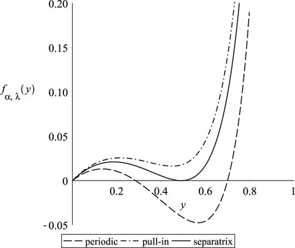
Figure 3. The separatrix occurs when the potential function $f_{\alpha ,\lambda }(y)$ is tangent to the horizontal axis.

Note that Equation 42 has at most four roots. One root is negative and lies outside the interval (0,1), while another root occurs at $y=0$. Within the interval (0,1), there are at most two roots. Moreover, the cubic function

$h_{\alpha ,\lambda }\left(y\right)=\frac{2}{3}\alpha y^3-\left(\frac{2}{3}\alpha -1\right)y^2-y+2\lambda (43)$

intersects the horizontal axis at the same points as $f_{\alpha ,\lambda }(y)$, except for 0. Equation 43 is tangent to the horizontal axis if both $h_{\alpha ,\lambda }(y^{*})=0$ and $h_{\alpha ,\lambda }^{\prime }(y^{*})=0$ for some $y^{*}\in (\mathrm{0,1})$. Then,

$h_{\alpha ,\lambda }^{\prime }\left(y\right)=2\alpha y^2-2\left(\frac{2}{3}\alpha -1\right)y-1=0$

yields

$y_{\mathrm{1,2}}^{*}=\frac{\left(\frac{2}{3}\alpha -1\right)\pm \sqrt{{\left(\frac{2}{3}\alpha -1\right)}^2+2\alpha }}{2\alpha },$

where only

$y^{*}=\frac{\left(\frac{2}{3}\alpha -1\right)+\sqrt{{\left(\frac{2}{3}\alpha -1\right)}^2+2\alpha }}{2\alpha }$

lies within the interval (0,1). Consequently, the system exhibits an oscillatory or periodic solution if $h_{\alpha ,\lambda }(y^{*})\le 0$ for some positive parametric values of $\alpha$ and $\lambda$. This condition can be expressed as

$h_{\alpha ,\lambda }\left(y^{*}\right)=\frac{1}{162{\alpha }^2}\left(-8{\alpha }^3+\alpha \left(27-6\nu \right)-9\left(-3+\nu \right)-2{\alpha }^2\left(9+2\nu -162\lambda \right)\right)\le 0,$

where

$\nu =\sqrt{9+6\alpha +4{\alpha }^2}.$

Rearranging the inequality and expressing $\lambda$ in terms of $\alpha$ gives

$\lambda \le -\frac{1}{324{\alpha }^2}\left(-8{\alpha }^3+\alpha \left(27-6\nu \right)-9\left(-3+\nu \right)-2{\alpha }^2\left(9+2\nu \right)\right)≕\kappa \left(\alpha \right).(44)$

The operational diagram for the MEMS graphene oscillator is presented in Figure 4. The parameter values $(\alpha ,\lambda )$ located above the separatrix $\kappa (\alpha )$ defined by Equation 44 lead to pull-in solutions. As a result, the exact formula for dynamic pull-in voltage can be expressed as follows:

$V_{\mathit{pull-in}}=\sqrt{\frac{2k_1{\left(d+\frac{h}{{\epsilon }_r}\right)}^3\kappa \left(\alpha \right)}{{\epsilon }_{0}S}}.$

Figure 4

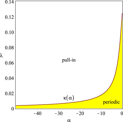
Figure 4. Parameter regions for pull-in and periodic solutions.

Another crucial parameter in MEMS devices is the pull-in time, which represents the time required for the system to collapse. The pull-in time can be obtained from Equation 41, where we express the velocity of the beam’s tip at a given position and parameter value $\lambda$ as follows:

$\dot{y}=\frac{dy}{dt}=\sqrt{-y^2-\frac{2}{3}\alpha y^3+\frac{2\lambda }{\left(1-y\right)}-2\lambda }.(45)$

Subsequently, the pull-in time, denoted as $t_{\text{pull}-\text{in}}$, is determined by

$t_{\text{pull}-\text{in}}={\int }_0^1\frac{dy}{\sqrt{-y^2-\frac{2}{3}\alpha y^3+\frac{2\lambda }{\left(1-y\right)}-2\lambda }}.(46)$

The integration of this expression over the interval [0,1] corresponds to the distance that the beam’s tip needs to travel in order to reach the fixed electrode, thus leading to the occurrence of a pull-in phenomenon. In Figure 5, the effect of excitation parameter $\lambda$ on the pull-in time is illustrated for various values of $\alpha$. The pull-in time by Equation 46 decreases with increasing $\lambda$ at a fixed value of $\alpha$. Using a similar approach, we can determine the period of oscillation $T$ for our system by integrating $dt$ from Equation 45 over the interval $[0,y_{\mathit{max}}]$ and then multiplying the result by 2:

$T={\int }_0^{y_{\mathit{max}}}\frac{2dy}{\sqrt{-y^2-\frac{2}{3}\alpha y^3+\frac{2\lambda }{\left(1-y\right)}-2\lambda }}.(47)$

Figure 5

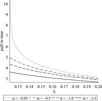
Figure 5. Pull-in times for various values of parameter $\alpha$.

Here, $y_{\mathit{max}}\in (\mathrm{0,1})$ represents the amplitude of oscillation, which corresponds to the root of the function $h_{\alpha ,\lambda }(y)$. The amplitude of oscillations is illustrated in phase diagrams and the corresponding plots of the potential energy function; see Figures 6–9.

Figure 6

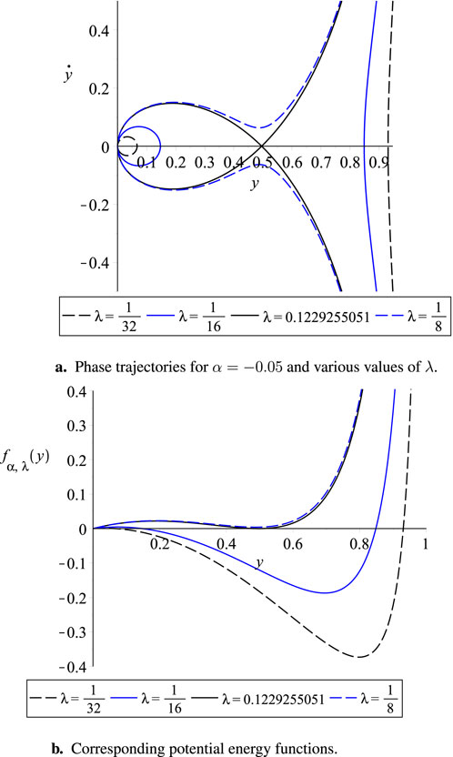
Figure 6. (a) Phase trajectories for $\alpha =-0.05$ and various values of $\lambda$ and (b) corresponding potential energy functions.

Figure 7

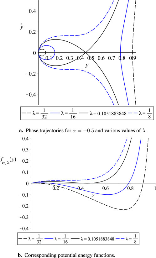
Figure 7. (a) Phase trajectories for $\alpha =-0.5$ and various values of $\lambda$ and (b) corresponding potential energy functions.

Figure 8

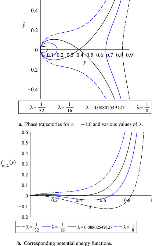
Figure 8. (a) Phase trajectories for $\alpha =-1.0$ and various values of $\lambda$ and (b) corresponding potential energy functions.

Figure 9

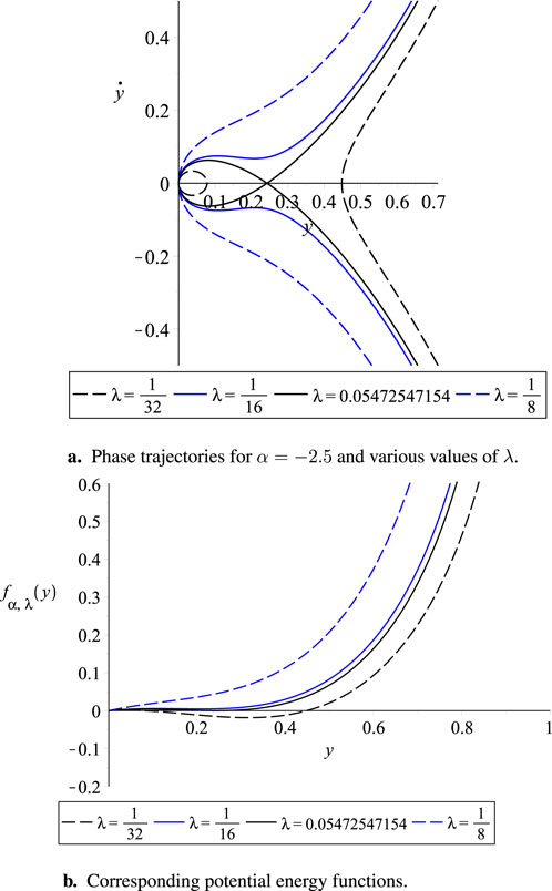
Figure 9. (a) Phase trajectories for $\alpha =-2.5$ and various values of $\lambda$ and (b) corresponding potential energy functions.

5.2 Time-dependent voltage

The pull-in phenomenon in a microelectromechanical system (MEMS) with a parallel-plate capacitor under time-dependent voltage $V(t)$ was studied by Kadyrov et al. [22], where $V(t)$ is expressed as

$V\left(t\right)=V_{DC}+V_{AC}\cos \left(\mathrm{\Omega }t\right),(48)$

with the forcing frequency $\mathrm{\Omega }$ and excitation period $T=\frac{2\pi }{\mathrm{\Omega }}$. They proposed a theorem that states the following: for a non-negative constant $c$, continuous real function $h(x)$ defined on $(-\infty ,1]$, and a periodic real function $V(t)$, the second-order nonlinear differential equation

$\ddot{y}+c\dot{y}+h\left(y\right)-\frac{V^2\left(t\right)}{{\left(1-y\right)}^2}=0(49)$

has a periodic solution if the equation

$h\left(y\right)=\frac{V_M^2}{{\left(1-y\right)}^2}$

has a root in (0,1), and it does not attain a periodic solution if the equation

$h\left(y\right)=\frac{V_m^2}{{\left(1-y\right)}^2}$

does not have any roots in $(-\infty ,1)$, but $h(y)$ has at least one real root within the interval $(-\infty ,1)$. Here, $V_m$ and $V_M$ represent the minimum and maximum amplitudes of $V(t)$, respectively, given by

$V_m=\underset{t\ge 0}{\min }|V\left(t\right)|\text{and}{V}_M=\underset{t\ge 0}{\max }|V\left(t\right)|.$

Our nondimensional model by Equation 39 is the special case of Equation 49 with $c=0$ and $h(y)=y+\alpha |y|y$. To prove the existence of periodic solutions, let us denote

${\lambda }_M=\underset{\tau \ge 0}{\max }|\lambda \left(\tau \right)|.$

According to the theorem, the second-order nonlinear and non-autonomous differential equation

$\ddot{y}+y+\alpha |y|y-\frac{\lambda \left(\tau \right)}{{\left(1-y\right)}^2}=0$

has a periodic solution provided that

$y+\alpha |y|y=\frac{{\lambda }_M}{{\left(1-y\right)}^2}$

has a root in (0,1). Let us define the function $f(y)$ as

$f_{\alpha }\left(y\right)=\left(y+\alpha |y|y\right){\left(1-y\right)}^2.$

Note that for $y\in (\mathrm{0,1})$,

$\left(y+\alpha |y|y\right){\left(1-y\right)}^2=\left(y+\alpha y^2\right){\left(1-y\right)}^2,$

Therefore,

$f_{\alpha }\left(y\right)=\left(y+\alpha y^2\right){\left(1-y\right)}^2\text{in}\left[\mathrm{0,1}\right).(50)$

By solving $f^{\prime }(y)=0$, we can find the critical points of Equation 50 that correspond to the values

$y_{\mathrm{1,2}}=\frac{2\alpha -3\pm \sqrt{4{\alpha }^2+4\alpha +9}}{8\alpha }\text{and}{y}_3=1.$

Then, using the second derivative test, we can find that $f_{\alpha }(y)$ has a local maximum at the smallest critical point $y_1=\frac{2\alpha -3+\sqrt{4{\alpha }^2+4\alpha +9}}{8\alpha }$ which belongs to the interval (0,1). It is worth noting that $f_{\alpha }(y_1)>0$ for all $\alpha$. Choosing $0<{\lambda }_M\le f_{\alpha }(y_1)=\mathcal{K}(\alpha )$ and recalling $f_{\alpha }(1)=0$, we have

$f_{\alpha }\left(1\right)-{\lambda }_M\le f_{\alpha }\left(y\right)-{\lambda }_M\le f_{\alpha }\left(y_1\right)-{\lambda }_M,$

where

$f_{\alpha }\left(1\right)-{\lambda }_M<0\text{and}{f}_{\alpha }\left(y_1\right)-{\lambda }_M\ge 0.$

Hence, the Intermediate Value theorem guarantees the existence of some $y^{*}$ in $(y_1,1)\subset (\mathrm{0,1})$ such that $f_{\alpha }(y^{*})-{\lambda }_M=0$. Then, based on the theorem, it can be concluded that Equation 55 admits a periodic solution. In order to have an oscillatory solution, the following condition for a choice of $\alpha$ and $\lambda$ must be satisfied:

$\lambda \le \frac{{\left(-3-6\alpha +\mu \right)}^2\left(-3+2\alpha +\mu \right)\left(5+2\alpha +\mu \right)}{4096{\alpha }^3}=\mathcal{K}\left(\alpha \right),$

with $\mu =\sqrt{9+4\alpha +4{\alpha }^2}$.

6 Simulation results

6.1 Constant voltage

In this section, we present numerical simulations of the normalized deflection of the beam’s free tip, denoted as $y(t)$, as a function of nondimensional time $t$. We analyze the behavior of the periodic solution $y(t)$ under the various sets of parameters $\lambda >0$ and $\alpha <0$. The simulations were conducted using Maple™ software [38], and the resulting deflection profiles are illustrated in Figures 10–13. The observed trends demonstrate the dependency of the deflection amplitude, frequency, and pull-in time on the excitation parameter $\lambda$ while keeping the parameter $\alpha$ fixed. Specifically, an increase in the value of $\lambda$ leads to a higher amplitude and longer period of deflection. Notably, the maximum deflection amplitude is attained when $\lambda$ approaches the threshold value $\kappa (\alpha )$. In Figures 10–13, the periodic solutions with the highest amplitude correspond to excitation value $\lambda =\kappa (\alpha )-10^{-3}$. Furthermore, as we decrease the value of $\alpha$, there is a corresponding increase in both the amplitude and period of $y(t)$, while the parameter $\lambda$ remains unchanged.

Figure 10

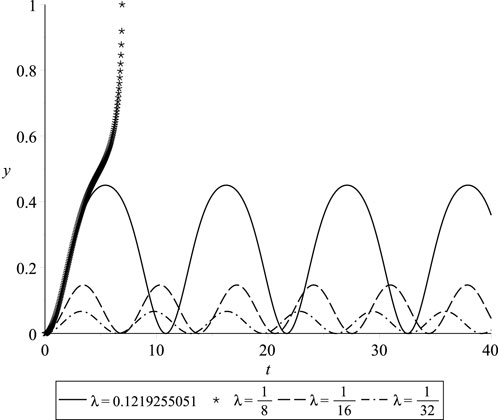
Figure 10. Profiles of periodic and pull-in solutions for $\alpha =-0.05$ and various values of $\lambda >0$ and $t_{\text{pull}-\text{in}}=6.9161$.

Figure 11

Figure 11. Profiles of periodic and pull-in solutions for $\alpha =-0.5$ and various values of $\lambda >0$ and $t_{\text{pull}-\text{in}}=3.0724$.

Figure 12

Figure 12. Profiles of periodic and pull-in solutions for $\alpha =-1$ and various values of $\lambda >0$ and $t_{\text{pull}-\text{in}}=4.2412$.

Figure 13

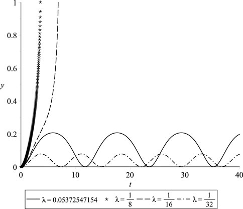
Figure 13. Profiles of periodic and pull-in solutions for $\alpha =-2.5$ and various values of $\lambda >0$, $t_{\text{pull}-\text{in}}=3.5571$, and $t_{\text{pull}-\text{in}}=6.8102$ for $\lambda =1/8$ and $\lambda =1/16$, respectively.

6.2 Time-dependent voltage

In this section, we will conduct an in-depth analysis of the resonance phenomenon in a cantilever beam that is subjected to a harmonic force. Depending on the frequency of harmonic excitation, the dynamic behavior of the system can be classified as primary and secondary resonance. Primary resonance refers to a dynamic behavior observed in a system when it is excited by a frequency that is close to its natural frequency. The dynamic response of the system becomes significantly amplified under primary resonance conditions, leading to large vibration amplitudes. On the other hand, secondary resonance occurs when the system is excited at frequencies that are different from its natural frequencies and are located relatively far from them [1]. However, for our analysis, we will specifically focus on primary resonance. For our analysis, we fix the value of $\alpha =-1.0$. The corresponding threshold value for excitation parameter ${\lambda }^{*}$ with DC voltage $V_{DC}$ is

${\lambda }^{*}=\kappa \left(\alpha \right)=0.08802549127.$

Recall that

$\lambda =\frac{{\epsilon }_0{V}_{DC}^{2}S}{2k_1{\left(d+\frac{h}{{\epsilon }_r}\right)}^3}.$

Let us denote

$\beta =\frac{{\epsilon }_{0}S}{2k_1{\left(d+\frac{h}{{\epsilon }_r}\right)}^3},$

and fix $\beta =0.01$. Then, the corresponding pull-in voltage equals

$V_{DC}=\sqrt{\frac{{\lambda }^{*}}{\beta }}=2.97.(51)$

The pull-in value of DC voltage indicates that, for the fixed values of $\alpha$ and $\beta$, the system excited by harmonic voltage by Equation 48 should undergo a DC voltage less than the pull-in voltage from Equation 51. Therefore, for dynamic analysis, we employ $V_{DC}=2.5$ and $V_{AC}=0.1$. Using Equation 47 and utilizing the fact that

$\mathrm{\Omega }=\frac{2\pi }{T}$

yields for $V_{AC}=0$ the natural angular frequency of the system as ${\omega }_n=0.7391982714$. As the forcing frequency $(\mathrm{\Omega })$ approaches the system’s natural resonant frequency, the system becomes instable, and then pull-in occurs. The results depicted in Figure 14 demonstrate that when the excitation frequency $\mathrm{\Omega }$ is selected to be close to the natural frequency ${\omega }_n$, the amplitude of the graphene cantilever beam’s vibration experiences a substantial increase compared to its behavior under constant voltage conditions. Letting the excitation frequency be precisely equal to the natural frequency, resonance occurs and leads to a substantial increase in the vibration amplitude of the graphene cantilever beam. However, this increment is accompanied by the occurrence of a pull-in instability scenario, wherein the free tip of the beam collapses into the fixed electrode; see Figure 15.Figures 14, 15 show an oscillatory behavior for the case of $\mathrm{\Omega }=0$. The solution for $\mathrm{\Omega }=0$ is periodic because the point $(\alpha ,\lambda )$ lies below the separatrix curve $\kappa (\alpha )$; see Figure 4.

Figure 14

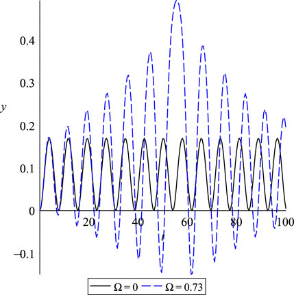
Figure 14. Dynamic response of a graphene cantilever beam under constant voltage and harmonic excitation near natural angular frequency.

Figure 15

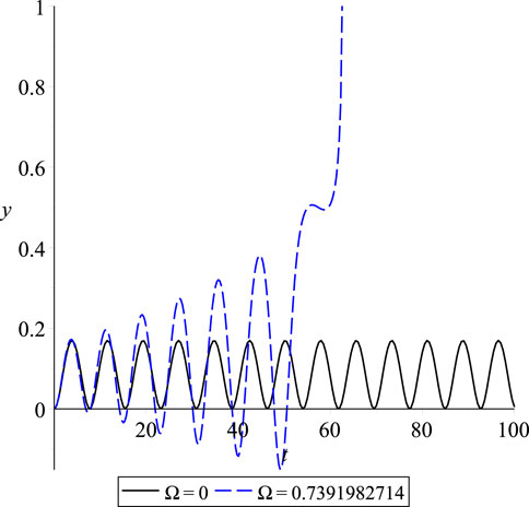
Figure 15. Dynamic response of a graphene cantilever beam under constant voltage and harmonic excitation at natural angular frequency, $t_{\text{pull}-\text{in}}=62.56$.

7 Conclusion and outlooks

In this study, a comprehensive analysis of the static and dynamic behavior of a graphene cantilever beam subjected to electrostatic actuation at its free tip was conducted. First, an analytical solution for the nonlinear static problem was derived, and its consistency with the classical linear solution was demonstrated in the limit where the second-order elastic stiffness constant $D$ approaches 0. Next, the dynamic pull-in conditions of the system were investigated for two cases: under constant and harmonically excited voltages. Analytical predictions were rigorously validated through numerical simulations presented in Section 6. For the case of constant voltage excitation, the system exhibited periodic solutions when the parameter values $\alpha$ and $\lambda$ lay below the separatrix curve, as illustrated in Figure 4. Conversely, pull-in phenomena occurred when these parameters exceeded the separatrix curve. The dependency of the deflection amplitude, frequency, and pull-in time on the excitation parameter $\lambda$ for a fixed value of $\alpha$ was demonstrated in this section. Additionally, it was observed that the maximum deflection amplitude occurred immediately below the separatrix value for the given $\alpha$. Furthermore, simulations of the cantilever beam under harmonic load excitation revealed that selecting an excitation frequency near the resonant frequency of the beam could lead to structural collapse even though the parametric values were below the pull-in conditions. Our findings in this paper can be useful in future MEMS design. Experimental validations and comparative study of alternative mass lumped models for graphene resonators are subjects of future research work. Precise models are crucial due to graphene resonators’ unique traits, and the homotopy perturbation method [43–45] is ideal for complex situations. As problems get intricate with non-linearities, it can break down equations, outperforming traditional methods.

Data availability statement

The original contributions presented in the study are included in the article/Supplementary Material; further inquiries can be directed to the corresponding author.

Author contributions

J-HH: conceptualization, methodology, writing – original draft, and writing – review and editing. QB: formal analysis, funding acquisition, writing – original draft, and writing – review and editing. Y-CL: conceptualization, writing – original draft, and writing – review and editing. DK: methodology, writing – original draft, and writing – review and editing. GE: formal analysis, investigation, writing – original draft, and writing – review and editing. YY: conceptualization, data curation, formal analysis, investigation, methodology, software, validation, visualization, writing – original draft, and writing – review and editing. PS: conceptualization, data curation, formal analysis, funding acquisition, investigation, methodology, project administration, resources, software, supervision, validation, visualization, writing – original draft, and writing – review and editing.

Funding

The author(s) declare that financial support was received for the research and/or publication of this article. PS and GE were supported by the Ministry of Education and Science of the Republic of Kazakhstan within the framework of Project AP19676969. QB was supported by Youth Top Talents Special Training Program of the “Yingcai Xingmeng” Project.

Conflict of interest

The authors declare that the research was conducted in the absence of any commercial or financial relationships that could be construed as a potential conflict of interest.

Generative AI statement

The author(s) declare that no Generative AI was used in the creation of this manuscript.

Publisher’s note

All claims expressed in this article are solely those of the authors and do not necessarily represent those of their affiliated organizations, or those of the publisher, the editors and the reviewers. Any product that may be evaluated in this article, or claim that may be made by its manufacturer, is not guaranteed or endorsed by the publisher.

Supplementary material

The Supplementary Material for this article can be found online at: https://www.frontiersin.org/articles/10.3389/fphy.2025.1551969/full#supplementary-material

References

1. Younis MI MEMS linear and nonlinear statics and dynamics, 20. Springer Science and Business Media (2011).

Google Scholar

2. Hanay MS, Kelber S, Naik A, Chi D, Hentz S, Bullard E, et al. Single-protein nanomechanical mass spectrometry in real time. Nat Nanotechnology (2012) 7:602–8. doi:10.1038/nnano.2012.119

PubMed Abstract | CrossRef Full Text | Google Scholar

3. Jensen K, Kim K, Zettl A. An atomic-resolution nanomechanical mass sensor. Nat Nanotechnology (2008) 3:533–7. doi:10.1038/nnano.2008.200

PubMed Abstract | CrossRef Full Text | Google Scholar

4. Steele GA, Hüttel AK, Witkamp B, Poot M, Meerwaldt HB, Kouwenhoven LP, et al. Strong coupling between single-electron tunneling and nanomechanical motion. Science (2009) 325:1103–7. doi:10.1126/science.1176076

PubMed Abstract | CrossRef Full Text | Google Scholar

5. Fuhrer MS, Lau CN, MacDonald AH. Graphene: materially better carbon. MRS Bull (2010) 35:289–95. doi:10.1557/mrs2010.551

CrossRef Full Text | Google Scholar

6. Pesin D, MacDonald AH. Spintronics and pseudospintronics in graphene and topological insulators. Nat Mater (2012) 11(5):409–16. doi:10.1038/nmat3305

PubMed Abstract | CrossRef Full Text | Google Scholar

7. Lee J-U, Yoon D, Cheong H. Estimation of young’s modulus of graphene by Raman spectroscopy. Nano Lett (2012) 12:4444–8. doi:10.1021/nl301073q

PubMed Abstract | CrossRef Full Text | Google Scholar

8. Li Y. Reversible wrinkles of monolayer graphene on a polymer substrate: toward stretchable and flexible electronics. Soft Matter (2016) 12:3202–13. doi:10.1039/c6sm00108d

PubMed Abstract | CrossRef Full Text | Google Scholar

9. Tomori H, Kanda A, Goto H, Ootuka Y, Tsukagoshi K, Moriyama S, et al. Introducing nonuniform strain to graphene using dielectric nanopillars. Appl Phys Express (2011) 4:075102. doi:10.1143/apex.4.075102

CrossRef Full Text | Google Scholar

10. Khan ZH, Kermany AR, Öchsner A, Iacopi F. Mechanical and electromechanical properties of graphene and their potential application in mems. J Phys D: Appl Phys (2017) 50:053003. doi:10.1088/1361-6463/50/5/053003

CrossRef Full Text | Google Scholar

11. Rüegg A, Lin C (2013). Bound states of conical singularities in graphene-based topological insulators. Phys Rev Lett 110(4). doi:10.1103/physrevlett.110.046401

PubMed Abstract | CrossRef Full Text | Google Scholar

12. Wang X, Tian H, Xie W, Shu Y, Mi W-T, Ali Mohammad M, et al. Observation of a giant two-dimensional band-piezoelectric effect on biaxial-strained graphene. NPG Asia Mater (2015) 7:e154. doi:10.1038/am.2014.124

CrossRef Full Text | Google Scholar

13. Ghosh S, Calizo I, Teweldebrhan D, Pokatilov EP, Nika DL, Balandin AA, et al. Extremely high thermal conductivity of graphene: prospects for thermal management applications in nanoelectronic circuits. Appl Phys Lett (2008) 92. doi:10.1063/1.2907977

CrossRef Full Text | Google Scholar

14. Balandin AA, Ghosh S, Bao W, Calizo I, Teweldebrhan D, Miao F, et al. Superior thermal conductivity of single-layer graphene. Nano Lett (2008) 8:902–7. doi:10.1021/nl0731872

PubMed Abstract | CrossRef Full Text | Google Scholar

15. Iacopi F, Brongersma S, Vandevelde B, O’Toole M, Degryse D, Travaly Y, et al. Challenges for structural stability of ultra-low-k-based interconnects. Microelectronic Eng (2004) 75:54–62. doi:10.1016/j.mee.2003.09.011

CrossRef Full Text | Google Scholar

16. Dai MD, Kim C-W, Eom K. Nonlinear vibration behavior of graphene resonators and their applications in sensitive mass detection. Nanoscale Res Lett (2012) 7:499–10. doi:10.1186/1556-276x-7-499

PubMed Abstract | CrossRef Full Text | Google Scholar

17. Li L, Yu F, Qin Q (2024) Interaction and manipulation for non-autonomous bright soliton solution of the coupled derivative nonlinear Schrödinger equations with Riemann–Hilbert method. Appl Mathematics Lett 149. doi:10.1016/j.aml.2023.108924

CrossRef Full Text | Google Scholar

18. Natsuki T, Shi J-X, Ni Q-Q. Vibration analysis of nanomechanical mass sensor using double-layered graphene sheets resonators. J Appl Phys (2013) 114. doi:10.1063/1.4820522

CrossRef Full Text | Google Scholar

19. Karličić D, Kozić P, Adhikari S, Cajić M, Murmu T, Lazarević M. Nonlocal mass-nanosensor model based on the damped vibration of single-layer graphene sheet influenced by in-plane magnetic field. Int J Mech Sci (2015) 96:132–42. doi:10.1016/j.ijmecsci.2015.03.014

CrossRef Full Text | Google Scholar

20. Wei D, Liu Y, Elgindi MB. Some analytic and finite element solutions of the graphene Euler beam. Int J Computer Mathematics (2014) 91:2276–93. doi:10.1080/00207160.2013.871784

CrossRef Full Text | Google Scholar

21. Anjum N, He J-H. Nonlinear dynamic analysis of vibratory behavior of a graphene nano/microelectromechanical system. Math Methods Appl Sci (2020). doi:10.1002/mma.6699

CrossRef Full Text | Google Scholar

22. Kadyrov S, Kashkynbayev A, Skrzypacz P, Kaloudis K, Bountis A. Periodic solutions and the avoidance of pull-in instability in nonautonomous microelectromechanical systems. Math Methods Appl Sci (2021) 44:14556–68. doi:10.1002/mma.7725

CrossRef Full Text | Google Scholar

23. Skrzypacz P, Kadyrov S, Nurakhmetov D, Wei D. Analysis of dynamic pull-in voltage of a graphene mems model. Nonlinear Anal Real World Appl (2019) 45:581–9. doi:10.1016/j.nonrwa.2018.07.025

CrossRef Full Text | Google Scholar

24. Wei D, Nurakhmetov D, Aniyarov A, Zhang D, Spitas C. Lumped-parameter model for dynamic monolayer graphene sheets. J Sound Vibration (2022) 534:117062. doi:10.1016/j.jsv.2022.117062

CrossRef Full Text | Google Scholar

25. Omarov D, Nurakhmetov D, Wei D, Skrzypacz P. On the application of Sturm's theorem to analysis of dynamic pull-in for a graphene-based MEMS model. Appl Comput Mech (2018) 12. doi:10.24132/acm.2018.413

CrossRef Full Text | Google Scholar

26. Qing Q, Li L, Fajun Y (2024) Non-autonomous exact solutions and dynamic behaviors for the variable coefficient nonlinear Schrödinger equation with external potential. Physica Scripta 100(1). doi:10.1088/1402-4896/ad9870

CrossRef Full Text | Google Scholar

27. Varadan VK, Vinoy KJ, Jose KA. RF MEMS and their applications. John Wiley and Sons (2003).

Google Scholar

28. He J-H. Periodic solution of a micro-electromechanical system. Facta Universitatis, Ser Mech Eng (2024) 187–98. doi:10.22190/fume240603034h

CrossRef Full Text | Google Scholar

29. He J-H, Yang Q, He C-H, Alsolami AA. Pull-down instability of the quadratic nonlinear oscillators. Facta Universitatis, Ser Mech Eng (2023) 21:191–200. doi:10.22190/fume230114007h

CrossRef Full Text | Google Scholar

30. Li L, Fajun Y (2024). The fourth-order dispersion effect on the soliton waves and soliton stabilities for the cubic-quintic gross–pitaevskii equation, Chaos, Solitons and Fractals 179. doi:10.1016/j.chaos.2023.114377

CrossRef Full Text | Google Scholar

31. Skrzypacz P, Wei D, Nurakhmetov D, Kostsov EG, Sokolov AA, Begzhigitov M, et al. Analysis of dynamic pull-in voltage and response time for a micro-electro-mechanical oscillator made of power-law materials. Nonlinear Dyn (2021) 105:227–40. doi:10.1007/s11071-021-06653-3

CrossRef Full Text | Google Scholar

32. Poggetto VFD, Pal R, Pugno N, Miniaci M (2024). Topological bound modes in phononic lattices with nonlocal interactions. Int J Mech Sci 281. doi:10.1016/j.ijmecsci.2024.109503

CrossRef Full Text | Google Scholar

33. Lee C, Wei X, Kysar JW, Hone J. Measurement of the elastic properties and intrinsic strength of monolayer graphene. Science (2008) 321:385–8. doi:10.1126/science.1157996

PubMed Abstract | CrossRef Full Text | Google Scholar

34. Lu Q, Huang R. Nonlinear mechanics of single-atomic-layer graphene sheets. Int J Appl Mech (2009) 1:443–67. doi:10.1142/s1758825109000228

CrossRef Full Text | Google Scholar

35. Khan ZH, Kermany AR, Öchsner A, Iacopi F. Mechanical and electromechanical properties of graphene and their potential application in mems. J Phys D: Appl Phys (2017) 50:053003. doi:10.1088/1361-6463/50/5/053003

CrossRef Full Text | Google Scholar

36. Meirovitch L. Fundamentals of vibrations. Long Grove, Illinois: Waveland Press (2010).

Google Scholar

37. Skrzypacz P, Bountis A, Nurakhmetov D, Kim J. Analysis of the lumped mass model for the cantilever beam subject to grob’s swelling pressure. Commun Nonlinear Sci Numer Simulation (2020) 85:105230. doi:10.1016/j.cnsns.2020.105230

CrossRef Full Text | Google Scholar

38. Maplesoft. Maple user manual. Waterloo, Ontario: Maplesoft, a division of Waterloo Maple Inc. (1996).

Google Scholar

39. Chen Z, Gandhi U, Lee J, Wagoner R. Variation and consistency of young’s modulus in steel. J Mater Process Technology (2016) 227:227–43. doi:10.1016/j.jmatprotec.2015.08.024

CrossRef Full Text | Google Scholar

40. Howatson AM. Engineering tables and data. Springer Science and Business Media (2012).

Google Scholar

41. Hopcroft MA, Nix WD, Kenny TW. What is the young’s modulus of silicon? J Microelectromechanical Syst (2010) 19:229–38. doi:10.1109/jmems.2009.2039697

CrossRef Full Text | Google Scholar

42. Yajima S, Okamura K, Hayashi J. Structural analysis in continuous silicon carbide fiber of high tensile strength. Chem Lett (1975) 4:1209–12. doi:10.1246/cl.1975.1209

CrossRef Full Text | Google Scholar

43. Moussa B, Youssouf M, Abdoul Wassiha N, Youssouf P. Homotopy perturbation method to solve Duffing - Van der Pol equation. Advances in Differential Equations and Control Processes (2024) 31(3):299–315. doi:10.17654/0974324324016

CrossRef Full Text | Google Scholar

44. Alshomrani NAM, Alharbi WG, Alanazi IMA, Alyasi LSM, Alrefaei GNM, Al’amri SA, et al. Homotopy perturbation method for solving a nonlinear system for an epidemic. Advances in Differential Equations and Control Processes (2024) 31(3):347–355. doi:10.17654/0974324324019

CrossRef Full Text | Google Scholar

45. He JH, He CH, Alsolami AA. A good initial guess for approximating nonlinear oscillators by the homotopy perturbation method. Facta Univ Ser Mech Eng (2023) 21(1):21–29.

CrossRef Full Text | Google Scholar