Astrophysical constraints on the simulation hypothesis for this Universe: why it is (nearly) impossible that we live in a simulation

Introduction: The “simulation hypothesis” is a radical idea which posits that our reality is a computer simulation. We wish to assess how physically realistic this is, based on physical constraints from the link between information and energy, and based on known astrophysical constraints of the Universe.

Methods: We investigate three cases: the simulation of the entire visible Universe, the simulation of Earth only, or a low-resolution simulation of Earth compatible with high-energy neutrino observations.

Results: In all cases, the amounts of energy or power required by any version of the simulation hypothesis are entirely incompatible with physics or (literally) astronomically large, even in the lowest resolution case. Only universes with very different physical properties can produce some version of this Universe as a simulation.

Discussion: It is simply impossible for this Universe to be simulated by a universe sharing the same properties, regardless of technological advancements in the far future.

1 Introduction

The “simulation hypothesis” (SH) is a radical and thought-provoking idea with ancient and noble philosophical roots (for example, works by Descartes [1] and Berkeley [2]) and frequent echoes in the modern literature, which postulates that the reality we perceive is the creation of a computer program.

The modern version of the debate usually refers to an influential article by Bostrom [3], although several coeval science fiction movies contributed to popularizing this theme¹.

Despite its immense popularity, this topic has rarely been investigated scientifically because, at first sight, it might seem to be entirely out of the boundaries of falsifiability and hence relegated to social media buzz and noise.

A remarkable exception is the work by Beane et al. [4], who investigated the potentially observable consequences of the SH by exploring the particular case of a cubic spacetime lattice. They found that the most stringent bound on the inverse lattice spacing of the universe is $\sim 10^{-11}Ge{V}^{-1}$, derived from the high-energy cut-off of the cosmic ray spectrum. Interestingly, they proposed that the SH can be tested through the distributions of arrival direction of the highest energy cosmic rays through the detection of a degree of rotational symmetry breaking associated with the structure of the underlying lattice. Our work will also use ultra-high-energy cosmic rays and neutrinos to constrain the SH, although in a totally different way (e.g., Section 3.3).

Our starting point is that “ information is physical” [5, 6], and hence, any numerical computation requires a certain amount of power, energy, and computing time, and the laws of physics can clearly tell us what is possible to simulate and under which conditions. We can use these simple concepts to assess the physical plausibility—or impossibility—of a simulation reproducing the Universe² we live within, and even of some lower resolution version of it.

Moreover, the powerful physical nature of information processing allows us to even sketch the properties that any other universe simulating us must have in order for the simulation to be feasible.

This paper is organized as follows: Section 2 presents the quantitative framework we will use to estimate the information and energy budget of simulations; Section 3 will present our results for different cases of the SH; and Section 4 will critically assess some of the open issues in our treatment. Our conclusions are summarized in Section 4.6.

2 Methods: the holographic principle and information-energy equivalence

In order to assess which resources are needed to simulate a given system, we need to quantify how much information can be encoded in a given portion of the Universe (or in its totality). The holographic principle (HP) arguably represents the most powerful tool for establishing this connection. It was inspired by the modeling of black hole thermodynamics through the Bekenstein bound (see below), according to which the maximum entropy of a system scales within its encompassing surface rather than its enclosing volume. The HP is at the core of the powerful anti-de Sitter/conformal field theory correspondence (AdS/CFT), which links string theory with gravity in five dimensions with the quantum field theory of particles with no gravity on a four-dimensional space [7].

According to the HP, a stable and asymptotically flat spacetime region with the boundary of area $A$ is fully described by no more than $A/4$ degrees of freedom, or approximately 1 bit of information per Planck area, defined as Equation 1:

$l_p^2=G\hslash /c^3=2.59\cdot 10^{-66}{\mathrm{c}\mathrm{m}}^2.(1)$

where obviously $l_p=\sqrt{\hslash G/c^3}\sim 1.6\cdot 10^{-33}\mathrm{c}\mathrm{m}$ is the Planck scale. While in a local classical field theory description, there are far more degrees of freedom, the excitation of more than $A/4$ of these degrees of freedom will trigger gravitational collapse [8–10]. The total entropy contained with the holographic area $A$ follows from the generalized second law of thermodynamics, giving the Bekenstein bound, which applies to systems that are not strongly self-gravitating and whose energy is $E\approx M{c}^2$:

$S\le 2\pi k_B\frac{ER}{\hslash c}=A/4(2)$

In Equation 2, $R$ is the circumferential radius of the smallest sphere that fits around the matter system, assuming (nearly) Euclidean spacetime for simplicity, and $M$ is the mass of the system.

Next, we can use the classical information-entropy equivalence [11], which states that the minimum entropy production connected with any 1-bit measurement is given by Equation 3:

$H=k_b\mathrm{l}\mathrm{o}\mathrm{g}\mathrm{(2)}(3)$

where the log(2) reflects the binary decision. The amount of entropy for a single 1-bit measurement (or for any single 1-bit flip, i.e., a computing operation) can be greater than this fundamental amount but not smaller; otherwise, the second law of thermodynamics would be violated.

Therefore, the total information (in [bits]) that can possibly be encoded within the holographic surface $A$ is described by Equation 4:

$I_{\text{max}}=\frac{S}{H}=2\pi \frac{ER}{\hslash c\log \left(2\right)}.(4)$

How much energy is required to encode an arbitrary amount of information $(I)$ in any physical device? Computation and thermodynamics are closely related: in any irreversible³ computation, information must be erased, which is a physical reduction of the number of possible states of one physical register to 0. This necessarily leads to the decrease of entropy of the device used for computing, which must be balanced with an equal (or larger) increase in entropy of the Universe. Thermodynamics thus leads to the necessity of dissipating energy (via heat) to erase bits of information. The related cost of erasing one single bit is thus given by “Brioullin’s inequality,” Equation 5:

$\mathrm{\Delta }E\ge k_{B}T\log \left(2\right)(5)$

where $T$ is the (absolute) temperature where the energy is dissipated. If we apply this to the maximum information within the holographic sphere, we get Equation 6:

$E_{\text{I}}=2\pi k_{B}T\frac{ER}{\hslash c}(6)$

It is interesting to compute the ratio between the enclosed energy within the holographic surface, $E$, and the energy required to encode the same information, $E_I$, which scales as Equation 7:

$\chi =\frac{E_I}{E}\approx 27.5\frac{T}{1°\mathrm{K}}\frac{E}{1\mathrm{e}\mathrm{r}\mathrm{g}}\approx 0.04\frac{T}{1°\mathrm{K}}\frac{M}{m_p}(7)$

This physically means even at the low temperature of $\sim 1°K$ for computing, the minimum energy required to fully describe all internal degrees of freedom of the system becomes larger than the actual energy that the system contains, already for systems with a mass $M\sim 25m_p$, or more. This is enlightening, as it shows how the full simulation of any macroscopic (or astronomical) object is bound to require an astoundingly large amount of energy, which, in turn, allows us to assess the plausibility of the SH against known astrophysical bounds.

The exact bounds derived from Equation 4 depend on what systems are considered and on how $R$, $E$, and $S$ are defined [8, 14]. It must also be stressed that a key assumption in Bekenstein’s derivation formula is that the gravitational self-interaction of the system can be neglected, as highlighted by the fact that the Newton constant $G$ does not appear. Although this assumption is reasonably verified in the application explored in this work, we notice that the estimates for black holes can significantly differ [8].

3 Results: information requirements and energy bounds

3.1 Full simulation of the visible Universe

Based on the above formulas, we can first estimate the total information contained within the holographic surface with radius equal to the observable radius of the Universe, $R_U\approx 14.3\mathrm{G}\mathrm{p}\mathrm{c}$ (comoving), and assuming a critical density ${\rho }_c=8.5\cdot 10^{-30}\mathrm{g}/c{m}^3$, which is valid for a flat Universe at $z=0$ and using a value for the Hubble constant $H_0=67.4km/s/Mpc$. Equation 8 gives a total energy

$E_U=\frac{4\pi }{3}{R}_U^3{\rho }_c{c}^2\sim 2.7\cdot 10^{78}\mathrm{e}\mathrm{r}\mathrm{g}(8)$

Based on Equation 4, Equation 9 results in a maximum information of

$I_{\text{U}}\sim 3.5\cdot 10^{124}\mathrm{b}\mathrm{i}\mathrm{t}\mathrm{s}(9)$

which results into an ecoding energy given by Equation 10:

$E_{\text{I,\hspace{0.17em}U}}\sim 8.9\cdot 10^{108}\mathrm{e}\mathrm{r}\mathrm{g}(10)$

Assuming a computing temperature equal to the microwave background temperature nowadays $(T_{\text{CMB}}=2.7°(1+z)\mathrm{K})$. A summary of the key quantities of energy and information required for this simulation (as well as for the following lower resolution cases) is given in Table 1.

Table 1

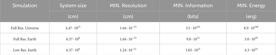
Table 1. Summary of the size, resolution, memory, and energy requirements of the tested simulation hypotheses.

As anticipated, because $E_{\text{I,U}}\gg E_U$, there is simply not enough energy within the entire observable Universe to simulate another similar universe down to its Planck scale, in the sense that there are not even remotely available resources to store the data to even begin the simulation. Therefore, the SH applied to the entire Universe is entirely rejected based on the unimaginable amount of energy it requires.

As noted above, slightly different estimates for the total information content of the Universe can be obtained by replacing the Bekenstein bound with the Hawking–Bekenstein formula, which computes the entropy of the Universe if that would be converted into a black hole, as in Equation 11:

$I_{\text{max}}^{\prime }=\frac{G{M}^2}{\hslash c}\sim 2.0\cdot 10^{124}\mathrm{b}\mathrm{i}\mathrm{t}\mathrm{s}(11)$

which is in line with similar estimates in the recent literature (Egan and Lineweaver [15], once we rescaled the previous formula for the volume within the cosmic event horizon rather than from the volume within the observable Universe; see also Profumo et al. [16] for a more recent estimate) and obviously incredibly larger than the amount of information that is generated even by the most challenging “cosmological” simulations produced to-date in astrophysics (e.g., $\sim 1.6\cdot 10^{13}\mathrm{b}\mathrm{i}\mathrm{t}\mathrm{s}$ of raw data in the Illustris-1 simulation, Vogelsberger et al. [17]).

This leads to the FIRST CONCLUSION: simulating the entirety of our visible Universe at full resolution (i.e., down to the Planck scale) is physically impossible.

3.2 Full simulation of planet Earth

Next, we can apply the same logic to compute the total memory information needed to describe our planet ($R_{\oplus }=6.37\cdot 10^8\mathrm{c}\mathrm{m}$, $M_{\oplus }=5.9\cdot 10^{27}\mathrm{g}$, and $E_{\oplus }=M_{\oplus }{c}^2=5.46\cdot 10^{48}\mathrm{e}\mathrm{r}\mathrm{g}$). We assume here that a planet is the smallest system that “the simulator” must model to recreate the daily experience that humankind collectively considers reality⁴.

Again, based on Equation 4, we get Equation 12:

$I_{\text{max},\oplus }=9.81\cdot 10^{74}\mathrm{b}\mathrm{i}\mathrm{t}\mathrm{s}(12)$

and for the total energy needed to code this information, Equation 13:

$E_{\text{max},\oplus }=2.55\cdot 10^{59}\mathrm{e}\mathrm{r}\mathrm{g}(13)$

assuming, very optimistically (as it will be discussed later), that $T=T_{\text{CMB}}$. The amount of energy required to even start the simulation of our planet is enormous, and it can be easily put into astrophysical context:

$•$ this is of the same order as the rest-mass energy of globular clusters like Palomar2 ($M_{gc}\sim 3.3\cdot 10^5{M}_{\odot }$, for example Baumgardt and Hilker [18]): $E_{\text{rm,\hspace{0.17em}gc}}=M_{\text{gc}}{c}^2\approx 5.6\cdot 10^{59}\mathrm{e}\mathrm{r}\mathrm{g}$;

$•$ this is also of the order of the potential binding energy of the halo of our Galaxy ($M_{\text{gal}}\sim 1.3\cdot 10^{12}{M}_{\odot }$ and $R_{\text{gal}}=287\mathrm{k}\mathrm{p}\mathrm{c}$, for example, Posti and Helmi [19]): $U_{\text{rm,\hspace{0.17em}gal}}\sim 3G{M}_{\text{gal}}^2/(5R_{\text{gal}})\sim 3.1\cdot 10^{59}erg$.

Therefore, the initialization of a complete simulation of “just” a planet like Earth requires either converting the entire stellar mass of a typical globular cluster into energy or using the equivalent energy necessary to unbind all stars and matter components in the Milky Way.

Elaborating on the implausibility of such a simulation, based on its energy cost, is straightforward: while this is indeed the requirement simply to begin the simulation, roughly the same amount of energy needs to be dissipated for each timestep of the simulation. This means that already after $\sim 10^6$ timesteps, the required energy is equivalent to the entire rest-mass energy of the Milky Way or roughly to the total potential energy of the most massive clusters of galaxies in the Universe.

Moreover, while the minimum mass required to contain this information corresponds to a black hole mass prescribed by Equation 11, which gives $\sim 0.32M_{\odot }$ using $I_{\text{max},\oplus }$, the actual energy required to encode the entire amount of bits, $E_{\text{max},\oplus }$, can at most be confined at within a radius corresponding to the Schwarzschild radius given by Equation 14:

$R_S=\frac{2G{E}_{\text{max},\oplus }}{c^4}\sim 4.95\cdot 10^9\mathrm{c}\mathrm{m}(14)$

which is 70% of the radius of Jupiter $(R_J=6.99\cdot 10^9\mathrm{c}\mathrm{m})$, meaning that a planetary-sized computer must be deployed for this simulation. The equivalent mass enclosed within such a radius will, of course, be very large: $M_{\text{max},\oplus }=E_{\text{max},\oplus }/c^2=1.68\cdot 10^5{M}_{\odot }$). Moreover, such a computing Jupiter must be continuously supplied with a similar amount of energy for each time step while all dissipated energy is somehow released outside of the system (and without raising the computing temperature).

Interestingly, such planetary-sized computers were theoretically explored by Sandberg [12], who presented a thorough study of all practical limitations connected to heat dissipation, computing power, connectivity, and bandwidth, arriving at a typical estimate of $\sim 10^{47}\mathrm{b}\mathrm{i}\mathrm{t}\mathrm{s}$ for a realistic Jupiter-sized computer. This is impressive, and yet 27 orders of magnitude fewer than what is required to encode the maximum information within the holographic surface containing our planet. Even setting aside the tremendous distance between the hypothetical and realistic memory capacity of such a colossal computer, the next problem is that concentrating so much mass and energy in such a limited volume will inevitably produce high levels of energy emission and heating, as in standard black holes and their related accretion disks.

If a black hole actively accretes matter, the kinetic temperature acquired by accreted matter is very large, and is given by Equation 15:

$T_{\text{acc}}\sim \frac{G{M}_{\text{max},\oplus }{m}_p}{3R_J{k}_B}\sim \frac{2m_p{c}^2}{3k_B},(15)$

That is, regardless of the actual mass and radius of the black hole into consideration, the temperature acquired by accreted particles is in the $\sim (m/m_p)\cdot 10^7\mathrm{K}$ regime for a generic particle with $m/m_p$ relative to the proton mass. Such temperature is manifestly much larger than the very optimistic cosmic microwave background (CMB) temperature we previously assumed to compute the minimum energy necessary to encode the full information of the simulation, that is, $T_{\text{acc}}\sim 10^7{T}_{\text{CMB}}$. From $E\propto k_{B}T{I}_{\text{MAX}}$ (Equation 4), it follows that the actual energy requirement is a factor of $\sim 10^7$ larger, even in the most optimistic configuration, requiring now a computer with radius $\sim 5\cdot 10^{17}\mathrm{c}\mathrm{m}$, that is, $\sim 0.16$ parsecs.

This leads to a SECOND CONCLUSION: simulating planet Earth at full resolution (i.e., down to the Planck scale) is practically impossible, as it requires access to a galactic amount of energy.

3.3 Low-resolution simulations of Planet Earth

Next, we shall explore the possibility of “partial” or “low-resolution” simulations of planet Earth, in which the simulation must only resolve scales that are routinely probed by human experiments or observations while using some sort of “subgrid” physics for any smaller scale.

The Planck scale $l_p$ is at the core of physics as we know it, but it is not a directly measurable scale by any means. In the framework of the SH, it is well conceivable that $l_p$ appears in the equations of our physics but that the simulation instead effectively works by discretizing our reality at a much coarser scale, thus providing a “low-resolution” simulation⁵.

What is the smallest scale, $\mathrm{\Delta }{x}_{\text{min}}$, that a realistic simulation of our planet should resolve in order for the simulation not to be incompatible with available human experiments or observations made on the planet?

High-energy physics, through the De Broglie relation, $\lambda =hc/E\sim h/p$, establishes an effective link between observed energy particle phenomena and spatial length-scales. So, the smallest resolution that the simulation must have depends on the highest energies routinely probed by human experiments. On Earth, the smallest high-energy scale probed by man-made experiments is in the $\sim 10^{-16}\mathrm{c}\mathrm{m}$ ballpark based on the particle collision energy scale reached with the Large Hadron Collider (LHC) [20]. However, this is true only limited to the portion of the terrestrial surface where the LHC is deployed (i.e., a ring of 27 km at most 200 m below sea level).

A much larger energy scale is probed by the detection of ultra-high-energy cosmic rays (UHECRs) as they cross our atmosphere and trigger the formation of observable Cherenkov radiation and fluorescent light [21, 22]. Observed UHECRs are characterized by a power-law distribution of events, and the largest energy ever recorded for an UHECR is $\sim 3\cdot 10^{20}\mathrm{e}\mathrm{V}$ (1991, the “Oh my god particle,” for example, Bird et al. [23]) while the second exceeded the $\sim 2.4\cdot 10^{20}\mathrm{e}\mathrm{V}$ range (2022, the “Amaterasu” particle, for example, Unger and Farrar [24]). The precise determination of “very energetic” is subject to absolute energy calibration uncertainties, also due to their uncertain composition; hence, we can use $E_{\text{UHECR}}=10^{20}eV=1.6\cdot 10^8\mathrm{e}\mathrm{r}\mathrm{g}$ as a conservative limit. This yields a length scale ${\lambda }_{\text{UHECR}}\sim 1.2\cdot 10^{-24}\mathrm{c}\mathrm{m}$. However, a hardcore proponent of the SH might still argue that this spatial scale is not really the most stringent experimental limit on the minimum spatial scale of the global Earth simulation because UHECRs probe only the last $\sim 10^2\mathrm{k}\mathrm{m}$ of air above the ground level, where particle cascades and airshowers are triggered by the interaction between UHECRs and air molecules. Hence, the simulator might keep most of the simulated volume of our planet at a much lower level of spatial resolution to limit computing resources. Indeed, the best resolution that is currently sampled for the interior of Earth, based on the advanced analysis of seismic shear waves diffracting along the core-mantle boundary, is “just” on the order of $\sim 10^2\mathrm{k}\mathrm{m}$ [25, 26].

Luckily, high-energy astrophysics still comes to the rescue due to the detection of very high-energy extragalactic neutrinos crossing the inside of our planet. Since the first discovery of energetic neutrinos by the IceCube observatory [27, 28], the existence of a background radiation of neutrinos, likely of extragalactic origin, in the $10\mathrm{T}\mathrm{e}\mathrm{V}-2PeV$ energy range, has been firmly established. Such neutrinos are very likely produced in external galaxies, even if the exact mechanism is highly uncertain [29–31]. In any case, the maximum energy scale probed so far reaches approximately $E_{\nu }\sim 10^{17}\mathrm{e}\mathrm{V}$ [32]; that is, lower than the maximum energy reached by UHECRs and in line with theoretical expectations by likely production mechanisms at the source. Unlike UHECRs, however, neutrinos cross our planet entirely because they are extremely weakly interacting with anything else. As a matter of fact, the IceCube observatory is more sensitive to events that are produced on the other side of the planet, with respect to its location on the South Pole, as this reduces the contamination by lower energy neutrinos of atmospheric or solar origin. Therefore, the established detection of this event can be used to constrain the minimum length scale which must be effectively adopted by any low-resolution simulation of our planet: ${\lambda }_{\nu }=hc/E_{\nu }\sim 1.2\cdot 10^{-21}\mathrm{c}\mathrm{m}$⁶. A simulation with an effective resolution coarser than this will be incompatible with our experimental data on neutrinos. Less straightforward is how to use this knowledge to estimate the information required for such a reduced-resolution simulation of planet Earth, using the holographic principle as before. The most conservative choice appears to be to still apply the HP approach but rescale the application of Equation 4 to the minimum element of area possible in the low-resolution simulation $(\propto {\lambda }_{\nu }^2)$, instead of the Planck area (Equation 1). Therefore, the minimum necessary information to be encoded follows from rescaling Equation 12 into Equation 16 for the ratio of the two areas:

$I_{\oplus ,\mathrm{l}\mathrm{o}\mathrm{w}}\approx I_{\text{max},\oplus }\cdot \frac{l_p^2}{{\lambda }_{\nu }^2}\approx 1.65\cdot 10^{51}\mathrm{b}\mathrm{i}\mathrm{t}\mathrm{s}.(16)$

Equation 17 gives a minimum encoding energy:

$E_{\oplus ,\mathrm{l}\mathrm{o}\mathrm{w}}=4.31\cdot 10^{35}\mathrm{e}\mathrm{r}\mathrm{g}(17)$

if we very conservatively use $T=T_{\text{CMB}}$ as above (which we are going to relax later on).

At face value, this energy requirement is far less astronomical than the previous one: it corresponds to the conversion into the energy of $\approx 2.4\cdot 10^{-19}{M}_{\odot }$ or $\approx 7.9\cdot 10^{-14}{M}_{\oplus }$ $(\sim 4.8\cdot 10^{14}\mathrm{g})$. This is still equal to the total energy radiated by the Sun in 2 minutes, considering the solar constant $(L_{\odot }\sim 3.8\cdot 10^{33}\mathrm{e}\mathrm{r}\mathrm{g}/s)$, yet it is an amount of energy that a fairly advanced civilization might access to.

Equation 11 gives the size of the minimum black hole capable of storing $I_{\oplus ,\mathrm{l}\mathrm{o}\mathrm{w}}$: $M_{\text{BH,low}}=4.4\cdot 10^{-13}{M}_{\odot }$. The radius relative to this mass is also fairly small: $R_{\text{BH,low}}=1.3\cdot 10^{-7}\mathrm{c}\mathrm{m}$. Therefore, while the total energy required for the initial encoding of the simulation’s data is still immense by modern human standards, it is tiny in astrophysical terms. However, we will next show that the only way to process the data of such simulation to advance it at sufficient speed requires access to unattainably large computing power, which makes this last low-resolution scenario impossible, too.

We largely used here the seminal work by Lloyd [13] for the computing capabilities of black holes. The ultimate compression limit of a black hole can provide in principle the most performing computing configuration for any simulation. Thus, by showing that not even in this case can the simulation be performed, we can argue about its physical impossibility. Based on the classical picture of black holes, no information is allowed to escape from within the event horizon. However, the quantum mechanical view is different as it allows, through the emission of Hawking radiation as black holes evaporate, to transfer some information on the outside. Following Lloyd [13], even black holes may theoretically be programmed to encode the information to be processed within their horizon. Then, an external observer, by examining the correlations in the Hawking radiation emitted as they evaporate, might be retrieving the result of the simulation outside. Even such a tiny black hole has a very long evaporation timescale: $t_{\text{ev}}\sim G^2{M}_{\text{BH,low}}^3/(3\hslash c^4\mathrm{k})$, with the constant $\mathrm{k}\sim 10^{-3}-10^{-2}$ depending on the species of particles composing the bulk of the BH mass, which gives $t_{\text{ev}}\ge 10^{35}\mathrm{s}$.

The temperature relative to the Hawking radiation for such a black hole is given by Equation 18:

$T_H\sim \frac{\hslash c^3}{8\pi G{M}_{\text{BH,\hspace{0.17em}low}}{k}_B}\sim 1.4\cdot 10^5\mathrm{K}.(18)$

Quantum mechanics constrains the maximum rate at which a system can move from one distinguishable quantum state to another. A quantum state with average energy $\bar{E}$ needs a time of order (at least) $\delta t\sim \pi \hslash /2\bar{E}$ to evolve into another orthogonal and distinguishable state. Hence, the number of logical operations per unit time (i.e., the computing frequency) that can be performed by a computing device is the inverse of the timescale from the Heisenberg uncertainty principle: $f\sim 1/\delta t\sim 2\bar{E}/(\pi \hslash )$. If such a black hole calculator uses all its storage memory, its maximum computing power per bit (i.e., the number of logical operations for each single bit) is estimated to be

$N_{\text{op}}=\frac{k_{B}2\log \left(2\right)\bar{E}}{\pi \hslash S}(19)$

In Equation 19, $S$ is the black hole entropy. The link between thermodynamic entropy and temperature here is given by $T={(\partial S/\partial \bar{E})}^{-1}$. By integrating the relationship linking $T$, $S$ and $\bar{E}$, we get $T=C\bar{E}/S$, in which $C$ is a constant of order unity that depends on the actual medium being used (e.g., $C=3/2$ for an ideal gas or $C=4/3$ for photons of a black-body spectrum). The dependence between the computing power and the working temperature is manifest: “the entropy governs the amount of information the system can register and the temperature governs the number of operations per bit per second it can perform,” as beautifully put by Lloyd [13].

Estimating the working temperature of such a device is not obvious. As an upper bound, we can use the temperature of accreted material at the event horizon of an astrophysical black hole from Equation 15 $(T\sim 10^7\mathrm{K})$ and get Equation 20:

$N_{\text{op}}\approx \frac{k_{B}2\log \left(2\right)T}{\pi \hslash }\sim 5.6\cdot 10^{17}\left[\mathrm{o}\mathrm{p}\mathrm{e}\mathrm{r}\mathrm{a}\mathrm{t}\mathrm{i}\mathrm{o}\mathrm{n}\mathrm{s}/bit/s\right].(20)$

By multiplying for the total number of bits encoded in such a black hole, Equation 21 gives its total maximum computing power:

$P_{\text{op}}\sim N_{\text{op}}\cdot I_{\oplus ,low}\sim 9.5\cdot 10^{68}\left[\mathrm{b}\mathrm{i}\mathrm{t}\mathrm{s}/s\right],(21)$

On the other hand, if the black hole does not accrete matter, the lowest temperature at the event horizon is the temperature relative to the Hawking radiation: $T_H\sim 1.4\cdot 10^5\mathrm{K}$ for this mass. Equation 22 thus gives:

$N_{\text{op}}^{\prime }\approx 8.0\cdot 10^{15}\left[\mathrm{o}\mathrm{p}\mathrm{e}\mathrm{r}\mathrm{a}\mathrm{t}\mathrm{i}\mathrm{o}\mathrm{n}\mathrm{s}/bit/s\right].(22)$

In this case, we get the total computing power:

$P_{\text{op}}^{\prime }\sim N_{\text{op}}^{\prime }\cdot I_{\oplus ,low}\sim 1.3\cdot 10^{67}\left[\mathrm{b}\mathrm{i}\mathrm{t}\mathrm{s}/s\right].(23)$

This computing power may seem immense, yet it is not enough to advance the low-resolution simulation of planet Earth in a reasonable wall-clock time. We notice that the minimum timestep that the simulation must resolve in order to consistently propagate the highest energy neutrinos we observe on Earth is $\mathrm{\Delta }t\approx {\lambda }_{\nu }/c\sim 4.1\cdot 10^{-32}\mathrm{s}$. In the extremely conservative hypothesis that only a few operations per bit are necessary to advance every bit of the simulation forward in time for a $\mathrm{\Delta }t$ timestep, $\sim O(10^{31})$ operations on every bit are necessary for the simulation to cover only 1 s of the evolution of our Universe. The two previous cases instead can at best achieve $\sim 8\cdot 10^{15}-5.6\cdot 10^{17}$ operations per bit per second, depending on the working temperature. In those conditions, a single second in the low-resolution simulation of planet Earth requires:

$•$ $t_{\text{CPU\hspace{0.17em}}}\sim 4.2\cdot 10^{13}\mathrm{s}$ of computing time, that is, $\sim 1.4\cdot 10^7\mathrm{y}\mathrm{r}$, using the computing power given by Equation 20;

$•$ $t_{\text{CPU}}\sim 3.0\cdot 10^{15}\mathrm{s}$ of computing time, that is, $\sim 1\cdot 10^8\mathrm{y}\mathrm{r}$ using the computing power given by Equation 22,

which are in both cases absurdly long wall-clock times. Therefore, an additional speed-up of order $\times 10^{15}-10^{17}$ (or larger) would be necessary to advance the low-resolution simulation of Earth faster than real time⁷. In this case, the necessary computing power will be simply impossible to collect:

$•$ $dE/dt\sim 1.1\cdot 10^{73}\mathrm{e}\mathrm{r}\mathrm{g}/s$ if the working temperature is $\sim 10^5\mathrm{K}$,

$•$ $dE/dt\sim 9.4\cdot 10^{74}\mathrm{e}\mathrm{r}\mathrm{g}/s$ if the working temperature is $\sim 10^7\mathrm{K}$,

which means converting into energy many more than all stars in all galaxies within the visible Universe (and using a black hole with mass $\sim 10^{-13}{M}_{\odot }$ for this). No known process can even remotely approach this power, and thus also this scenario appears absurd.

This leads us to the THIRD CONCLUSION: even the lowest possible resolution simulation of Earth (at a scale compatible with experimental data) requires geologically long timescales, making it entirely implausible for any purpose.

4 Discussion

Needless to say, in such a murky physical investigation, several assumptions can be questioned, and a few alternative models can be explored. Here, we review a few that appear to be relevant, even if it is anticipated that the enthusiasts of the SH will probably find other escape routes.

4.1 Can highly parallel computing make the simulation of the low-resolution Earth possible?

A reasonable question would be whether performing highly parallel computing could significantly reduce the computing time estimated at the end of Section 3.3. In general, if the required computation is serial, the energy can be concentrated in particular parts of the computer, while if it is parallelizable, the energy can be spread out evenly among the different parts of the computer.

The communication time across the black hole horizon $(t_{\text{com}}\sim 2R/c)$ is of the same order of the time to flip a single bit ($\sim \pi \hslash /(2\bar{E})$, see above); hence, in principle, highly parallel computing can be used here. However, the somewhat counter-intuitive result of Lloyd [13] is that the energy $E$ is divided among $N_{\text{proc}}$ processing units (each operating at a rate $\sim 2E/(\pi \hslash N_{\text{proc}})$) the total number of operations per second performed by the black hole remains the same: $\sim N_{\text{proc}}2E/(\pi \hslash N_{\text{proc}})=2E/(\pi \hslash )$, as in Section 3.3. This strictly follows from the quantum relation between computing time and spread in energy explored in Section 3.3. Thus, if the energy is allocated to a more parallel processor, the energy spread on which they operate gets smaller, and hence they run in a proportionally slower way. Finally, if the computing is spread to a configuration significantly less dense than a black hole by keeping the same mass, higher levels of parallelization can be used, but the computing time will increase as a black hole computer already provides the highest number of operations per bits per second (Equation 19).

4.2 What if the time stepping is not determined by neutrino observations?

What if (for reasons beyond what our physics can explain) high-energy neutrinos can be accurately propagated in the simulation with a time stepping much coarser than the one prescribed by $\mathrm{\Delta }t={\lambda }_{\nu }/c\sim 4.1\cdot 10^{-32}\mathrm{s}$? In this case, the next constraint to fulfil is still very small and given by the smallest time interval that humans could directly measure so far in the laboratory: this is $\mathrm{\Delta }{t}^{\prime }\approx 10^{-20}\mathrm{s}$ [33]. In this case, applying the same logic of Section 3.3, we get $t_{\text{CPU}}\sim 40-10^4\mathrm{s}$ depending on the computing temperature, which still means a simulation running several orders of magnitude slower than real time. Moreover, even in this scenario, the amount of power to process is (literally) out of this world: $dE/dt\sim k_{B}T\log (2)\cdot P_{\text{op}}\sim 10^{44}-10^{47}\mathrm{e}\mathrm{r}\mathrm{g}/s$ if we rescale Equations 21–23 for the new time rate. This power is astronomically large but not entirely impossible: mergers between massive clusters of galaxies, which are among the most energetic exchanges of matter in the Universe, “only” produce $\sim 10^{45}\mathrm{e}\mathrm{r}\mathrm{g}/s$ of power [34]. Distant quasars can radiate energy up to $\sim 10^{47}\mathrm{e}\mathrm{r}\mathrm{g}/s$ [35], while supernovae can release up to $\sim 10^{52}\mathrm{e}\mathrm{r}\mathrm{g}/s$, mostly in the form of energetic neutrinos and only in the first $\sim 1-10$ seconds of their explosion. A gamma ray burst from a hypernova can dissipate up to $\sim 10^{54}\mathrm{e}\mathrm{r}\mathrm{g}/s$ on a timescale of days [36]. Finally, the detection of gravitational waves by merging black holes (with masses of several tens of $M_{\odot }$) probed energy dissipation rates of several $\sim 10^{56}\mathrm{e}\mathrm{r}\mathrm{g}/s$ but is limited to the short timescale of the coalescence [37]. In any case, conveying in a steady way such a gigantic amount of energy through the microscopic black hole required for this very low-resolution scenario appears to be an impossible task.

4.3 What about quantum computing?

By exploiting the fundamental quantum properties of superposition and entanglement, quantum computers perform better than classical computers for a large variety of mathematical operations [38]. In principle, quantum algorithms are more efficient in using memory, and they may reduce time and energy requirements [39] by implementing exponentially fewer steps than classical programs. However, these important advantages compared to classical computers do not change the problems connected with the SH analyzed in this work, which solely arise from the relationship between spacetime, information density, and energy. According to the HP, the information bound used here is the maximum allowed within a given holographic surface with radius $R$, regardless of the actual technique used to reach this concentration of information or to process it. Moreover, our estimated computing power does not stem from the extrapolation of the current technological performances of classical computing, but it already represents the maximum possible performance obtained in the futuristic scenario in which a black hole can be used as the ultimate computing device. In summary, while quantum computing might, in principle, be the actual way to get to the maximum computing speed physically allowed at the scale of black holes (or in any other less extreme computing devices), this technology will not be able to beat the currently understood limits posed by physics.

4.4 What if the holographic principle does not apply?

One possibility is that the HP, for whatever reason, does not apply as a reliable proxy for the information content of a given physical system. It is worth reminding that the HP prescribes the maximum information content to scale with the surface, and not the volume, of a system; hence, it generally already provides a very low information budget estimate compared to all other proxies in which information scales with the volume instead. In this sense, the estimates used in this paper (including in the low-resolution simulation of Earth in Section 3.3) already appear as conservatively low quantities. If the HP is not valid, then a larger amount of bits can be encoded within a given surface with radius $R$ (in contradiction with our understanding of black hole physics). This will allow the usage of smaller computing devices, but at the same time, it will require even more computing power, making the SH even more implausible. On the other hand, while the HP prescribes the maximum information that can be encoded with a portion of spacetime, the actual evolution of the enclosed system might be described with fewer bits of information. For example, in recent work by Vazza [40, 41], we used mathematical tools from Information Theory [42, 43] to show that, on macroscopic scales, the statistical evolution of the cosmic web within the observable Universe can be encoded by using (only) $\sim 4\cdot 3\cdot 10^{16}\mathrm{b}\mathrm{i}\mathrm{t}\mathrm{s}$ of information. This is, of course, incredibly less than the $I_U\sim 3.5\cdot 10^{124}\mathrm{b}\mathrm{i}\mathrm{t}\mathrm{s}$ estimate quoted in Section 3.1 and following from the HP. However, the latter includes all possible evolution on all scales, down to the $l_p$ fundamental length, in which a plethora of multi-scale phenomena obviously happens. While the concept of “emergence” and efficiency of prediction for complex multi-scale phenomena is a powerful and useful tool to compress the information needed to describe physical patterns forming at specific scales [44], a full error-less simulation of a multi-scale system seems to require a much larger amount of information. In essence, we shall conclude that while it is conceivable that the actual information needed to fully capture the evolution of multi-scale phenomena emerging on different scales can be further reduced, it is implausible that the information budget quoted in this work can be reduced by several orders of magnitude.

4.5 Plot twist: a simulated Universe simulates how the real universe might be

Our results suggest that no technological advancement will make the SH possible in any universe that works like ours.

However, the limitations outlined above might be circumvented if the values of some of the fundamental constants involved in our formalisms are radically different than the canonic values they have in this Universe. Saying anything remotely consistent about the different physics operating in any other universe is an impossible task, let alone guessing which combinations of constants would still allow the development of any form of intelligent life. Nevertheless, for the sake of argument, we make the very bold assumption that in each of the explored variations, some sort of intelligent form of life can form and that it will be interested in computing and simulations. Under this assumption, we can then explore numerical changes to the values of fundamental constants involved in the previous modeling to see whether combinations exist that make at least a low-resolution simulation of our planet doable with limited time and energy.

So, in a final plot twist whose irony should not be missed, now this Universe (which might be a simulation) attempts to Monte Carlo simulate how the “real universe” out there could be for the simulation of this Universe to be possible. We assume that all known physical laws involved in our formalisms are valid in all universes, but we allow each of the key fundamental constants to vary randomly across realizations. For the sake of the exercise, we shall fix the total amount of information required for the low-resolution simulation of our planet discussed in Section 3.3 $(I_{\oplus ,low}=1.65\cdot 10^{51}\mathrm{b}\mathrm{i}\mathrm{t}\mathrm{s})$ and consider the Hawking temperature relative to the black hole which is needed in each universe to perform the simulation.

The simulation consists of a Monte Carlo exploration of the six-dimensional parameter space of the fundamental constants that entered our previous derivation: $G$, $m_p$, $k_B$, $c$, $\hslash$, to which we now add $H$, that is, the “Hubble–Lemaitre constant”⁸ to compute the cosmic time. From $10^6$ randomly drawn universes, we select all realizations in which the low-resolution simulation of our planet is “possible.” Each constant is free to randomly vary across 20 orders of magnitudes around its reference value. Our simplistic definition of possibility for the simulation here stems from two conditions:

$•$ the simulation can be run at least in real time, or faster than real time, in the universe where the simulation is produced. This means that a time interval of $1\mathrm{s}$ in this Universe is simulated in the equivalent of $1\mathrm{s}$ in the other universe. However, any other universe can have different evolutionary timescales than this one, depending on their $H$. By considering that $1\mathrm{s}\approx 3\cdot 10^{-18}{t}_U$, where $t_U$ is the age of this Universe, we require that one second of this Universe can be simulated in $\mathrm{\Delta }t=3\cdot 10^{-18}{t}_U$ of computing time in any other universe. To easily compute $t_U$, we assume for simplicity Einstein-de Sitter cosmology in every other universe, hence $t_U=2/(3H)$; here, $H$ is the Hubble–Lemaitre constant of other universes.

$•$ The power used to produce the simulation is “reasonable.” How can we guess what “reasonable” would be in any other universe? We cannot, of course, but for the sake of the exercise, we use $1GW$ of power as a goal: this is about the power provided by a modern nuclear reactor, and it is $\sim 10^2-10^3$ higher than the typical power consumed by the best high-performance computing center to-date. Thus, it represents some extreme power budget available to numerical astrophysicists of the remote future. As in the previous case, we must scale this power for the properties of other universes, and to do that, we consider that $1GW$ equates to $\sim 6.6\cdot 10^{18}$ protons ($\sim 10^{-33}$ of the mass of Earth) converted into energy in a second (where for the second, we again use the normalization of the previous step). Therefore, we assume that in any other universe, there are planets (or something conceptually equivalent) and that a very tiny fraction of their mass can be used to support computing.

In Figure 1, we give the results of the Monte Carlo simulation, in which we show samplings of the distribution of allowed combinations of constants, normalized to the value each of them has in this Universe. Although the exploration of the full 6-dimensional parameters space is complex, a few things can be noticed already. First, two well-correlated parameters here are $c$ and $h$: for a given value of the age of the universe, the computing timescale scales as $\propto h/T_H$, so if $c$ increases, the Hawking radiation temperature of the black hole increases too (lowering the computing timescale), while at the same time, proportionally larger values of $h$ are allowed. Another couple of correlated constants is $(c,G)$, which stems from the condition on the power: from this condition, it follows that $c^3/G\propto m_p$. Hence, an order of magnitude increase in $c$ must be compensated by a three-orders-of-magnitude increase in $G$ for a fixed value of $m_p$. Most of the other combinations of constants (e.g., $(m_p,k_B)$ and $(H,c)$ in Figure 1) show instead a lack of obvious correlation.

Figure 1

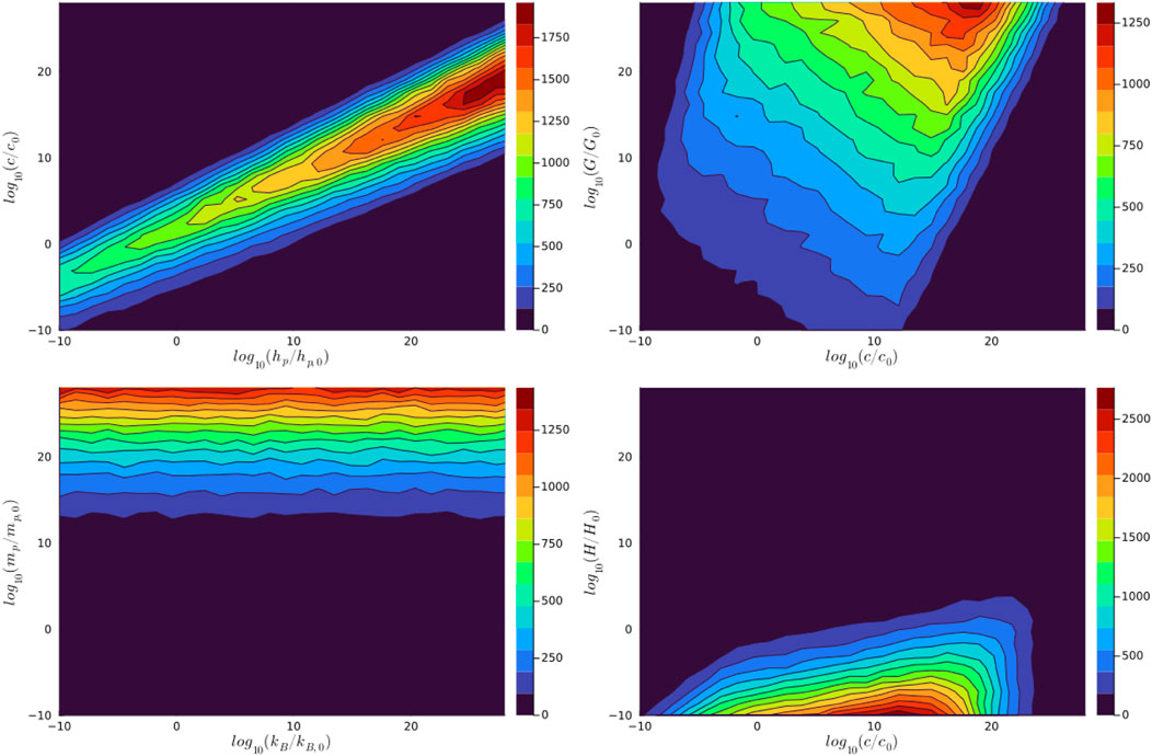
Figure 1. Examples of the distribution of allowed values of the fundamental constants (rescaled to their value in this Universe) necessary to perform a low-resolution simulation of Earth in other universes, as predicted with Monte Carlo simulations. Each axis gives the allowed value for each constant, normalized to its value in this Universe.

In general, this simulation shows that combinations of parameters exist to make the SH for a low-resolution version of planet Earth possible (and similarly, also for higher-resolution versions of the SH), although they require orders of magnitudes differences compared to the physical constants of this Universe. It is beyond the goal of this work to further elaborate whether any of the many possible combinations make sense, based on known physics, if they can support life, and whether those hypothetical forms of life will be interested in numerics and physics, as we are⁹.

4.6 What if the universe performing the simulation is entirely different from our Universe?

Guessing how conservation laws for energy and information apply in a universe with entirely different laws, or whether they should even apply in the first place, appears impossible, and this entirely prevents us from guessing whether the SH is possible in such a case. For example, hypothetical conscious creatures in the famous Pac-Man video game in the 1980s will simply be incapable of figuring out the constraints on the universe in which their reality is being simulated, even based on all the information they can gather around them. They would not guess the existence of gravity, for example; they would probably measure energy costs in “Power Pellets,” and they would not conceive the existence of a third dimension, or of an expanding spacetime, and so on. Even if they could ever realize the level of graininess of their reality and make the correct hypothesis of living in a simulation, they would never guess how the real universe (“our” Universe, if it is real indeed) functions in a physical sense. In this respect, our modeling shows that the SH can be reasonably well tested only with respect to universes that are at least playing according to the physics playbook—while everything else¹⁰ appears beyond the bounds of falsifiability and even theoretical speculation.

5 Conclusion

We used standard physical laws to test whether this Universe or some low-resolution version of it can be the product of a numerical simulation, as in the popular simulation hypothesis [3].

One first key result is that the simulation hypothesis has plenty of physical constraints to fulfil because any computation is bound to obey physics. We report that such constraints are so demanding that all plausible approaches tested in this work (in order to reproduce at least a fraction of the reality we humans experience) require access to impossibly large amounts of energy or computing power. We are confident that this conclusively shows the impossibility of a “Matrix” scenario for the SH, in which our reality is a simulation produced by future descendants, machines, or any other intelligent being in a Universe that is exactly the one we (think we) live in—a scenario famously featured in the “The Matrix” movie in 1999, among many others. We showed that this hypothesis is simply incompatible with all we know about physics, down to scales that have already been robustly explored by telescopes, high-energy particle colliders, and other direct experiments on Earth.

What if our reality is instead the product of a simulation, in which physical laws (e.g., fundamental constants) different from our reality are used? A second result of this work is that, even in this alienating scenario, we can still robustly constrain the range of physical constants allowed in the reality simulating us. In this sense, the strong physical link between computing and energy also offers a fascinating way to connect hypothetical different levels of reality, each one playing according to the same physical rules. In our extremely simplistic Monte Carlo scan of models with different fundamental constants, a plethora of combinations seems to exist, although we do not dare to guess which ones could be compatible with stable universes, the formation of planets, and the further emergence of intelligent life. The important point is that each of such solutions implies universes entirely different from this one. Finally, the question of whether universes with entirely different sets of physical laws or dimensionalities could produce our Universe as a simulation seems to be entirely outside of what is scientifically testable, even in theory.

At this point, we shall notice that a possible “simulation hypothesis,” which does not pose obvious constraints on computing, might be the solipsistic scenario in which the simulation simulates “just” the single activity of the reader’s brain (yes: you), while all the rest is a sophisticated and very detailed hallucination. In this sense, nothing is new from Renee Descartes’ “evil genius” or “Deus deceptor”—that is, for some reason, an entire universe is produced in a sort of simulation, only to constantly fool us—from its more modern version of “Boltzmann brains” [45]. Conversely, a more contrived scenario in which the simulation simulates only the brain activity of single individuals appears to quickly run into the limitations of the SH exposed in this work: a shared and consistent experience of reality requires a consistent simulated model of the world, which quickly escalates into a too-demanding model of planet Earth down to very small scales as soon as physical experiments are involved.

At this fascinating crossroad between physics, computing, and philosophy, it is interesting to notice that the last egotistic version of the SH appears particularly hard to test or debunk with physics, as the latter indeed appears to be entirely relying on the concept of a reality external to the observing subject—be it a real or a simulated one. However, the possibility of a quantitative exercise like the one attempted here also shows that the power of physics is otherwise immense, as even the most outlandish and extreme proposal about our reality must fall within the range of what physics can investigate, test, and debunk.

Luckily, even in the most probable scenario of all (the Universe is not a simulation), the number of mysteries for physics to investigate is still so immense that even dropping this fascinating topic cannot make science any less interesting.

Data availability statement

The raw data supporting the conclusions of this article will be made available by the authors, without undue reservation.

Author contributions

FV: Writing – original draft and writing – review and editing.

Funding

The author(s) declare that no financial support was received for the research and/or publication of this article.

Acknowledgments

I have used the Astrophysics Data Service (ADS) and arXiv preprint repository extensively during this project and for writing this article, the precious online Cosmological Calculator by E. Wright, and the Julia language for the simulations of Section 4.5. This peculiar investigation was prompted by a public conference given for the 40th anniversary of the foundation of Associazione Astrofili Vittorio Veneto, where the author took his first steps into astronomy. I wish to thank Maksym Tsizh and Chiara Capirini for their useful comments on the draft of the paper, and Maurizio Bonafede for useful suggestions on the geophysical analysis of the core-mantle boundary used in Section 3.3.

Conflict of interest

The author declares that the research was conducted in the absence of any commercial or financial relationships that could be construed as a potential conflict of interest.

Generative AI statement

The author(s) declare that no Generative AI was used in the creation of this manuscript.

Publisher’s note

All claims expressed in this article are solely those of the authors and do not necessarily represent those of their affiliated organizations, or those of the publisher, the editors and the reviewers. Any product that may be evaluated in this article, or claim that may be made by its manufacturer, is not guaranteed or endorsed by the publisher.

Footnotes

¹For example, it was the central topic of the 2016 Isaac Asimov Memorial Debate, featuring several astrophysicists and physicists: https://www.youtube.com/watch?v=wgSZA3NPpBs. This theme still periodically surges and generates a lot of “noise” on the web, indicating both the fascination it rightfully produces in the public and the difficulty of debunking it.

²As a sign of respect for what this astrophysicist honestly thinks is the only “real” Universe, which is the one we observe through a telescope, I will use the capital letter for this Universe—even if, for the sake of argument, is at times assumed to be only a simulation, being run in another universe.

³It must be noted that also reversible computation, with no deletion of bits or dissipation of energy, is possible. However, irreversible computation is unavoidable both for several many-to-one logical operations (AND or ERASE) as well as for error correction, in which several erroneous states are mapped into a single correct state [12, 13].

⁴For the sake of argument, because we surmise here the existence of a skilled simulator that somehow can use computing centers as large as a planet-sized black hole, we can concede with no difficulty that it can also create a consistent simulation of the experience of $\le 10^3$ astronauts who have temporarily left our planet and probed a larger portion of space. The simulator must also use a modest amount of extra computing resources to produce fake data to constantly keep astrophysicists and cosmologists busy while they think they are studying the universe.

⁵As a matter of fact, in almost any conceivable numerical simulation that is run in physics, the Planck constant and its associated length scale $l_p$ are at the core of many physical relations, and yet the effective spatial resolution of simulations is coarser than this by many orders of magnitude.

⁶Especially because we focus here on the simulation of Earth, a reasonable question would be whether such low-resolution simulation would still be capable of reproducing the observed biological process on the planet. A $\sim 10^{-21}\mathrm{c}\mathrm{m}$ length seems to be safely smaller than any process known to be relevant for biology, and thus, a hypothetical simulation using efficient subgrid modeling of processes below such resolution might correctly reproduce biology on Earth. If, instead, some biological processes will be shown to depend on $<10^{-21}\mathrm{c}\mathrm{m}$ scales, this can be used to revise our constraints on the smallest scale to be resolved by the simulation and call for an even more implausibly large amount of energy or power.

⁷It should also be considered that the time dilatation effect of general relativity will also introduce an additional delay factor between what is computed by the black hole and what is received outside, although the amount of the delay depends on where exactly the computation happens.

⁸Very likely to be named differently in any other universe.

⁹The full direct simulation of such cases, possibly down to the resolution at which conscious entities will emerge out of the simulation and start questioning whether their universe is real or simulated, is left as a trivial exercise to the reader.

¹⁰A possibility for such a model to work may be that all scientists are similar to “non playable characters” in video games, that is, roughly sketched and unconscious parts of the simulation, playing a pre-scripted role (in this case, reporting fake measurements).

References

1. Descartes R. Meditations on first philosophy. Ann Arbor: Caravan Books (1984).

Google Scholar

2. Berkeley GA. Treatise concerning the principles of human knowledge, 1734. Menston: Scolar Press (1734).

Google Scholar

3. Bostrom BN. Are we living in a computer simulation?. Philos Q (2003) 53:243–55. doi:10.1111/1467-9213.00309

CrossRef Full Text | Google Scholar

4. Beane SR, Davoudi Z, J Savage M. Constraints on the universe as a numerical simulation. Eur Phys J A (2014) 50:148. doi:10.1140/epja/i2014-14148-0

CrossRef Full Text | Google Scholar

5. Landauer R. Information is a physical entity. Physica A Stat Mech its Appl (1999) 263:63–7. doi:10.1016/S0378-4371(98)00513-5

CrossRef Full Text | Google Scholar

6. Landauer R. The physical nature of information. Phys Lett A (1996) 217:188–93. doi:10.1016/0375-9601(96)00453-7

CrossRef Full Text | Google Scholar

7. Maldacena JM. The large $N$ limit of superconformal field theories and supergravity. Adv Theor Math Phys (1998) 2:231–52. doi:10.4310/ATMP.1998.v2.n2.a1

CrossRef Full Text | Google Scholar

8. Bousso R. The holographic principle. Rev Mod Phys (2002) 74:825–74. doi:10.1103/RevModPhys.74.825

CrossRef Full Text | Google Scholar

9. Bekenstein JD. Black holes and information theory. Contemp Phys (2004) 45:31–43. doi:10.1080/00107510310001632523

CrossRef Full Text | Google Scholar

10. Suskind L, Lindesay J. An introduction to black holes, information and the string theory revolution: the holographic universe (2005).

Google Scholar

11. Szilard L. über die Entropieverminderung in einem thermodynamischen System bei Eingriffen intelligenter Wesen. Z Physik (1929) 53:840–56. doi:10.1007/BF01341281

CrossRef Full Text | Google Scholar

12. Sandberg A. The physics of information processing superobjects: daily life among the jupiter brains. J Evol Technology (1999) 5.

Google Scholar

13. Lloyd S. Ultimate physical limits to computation. Nature (2000) 406:1047–54. doi:10.1038/35023282

PubMed Abstract | CrossRef Full Text | Google Scholar

14. Page DN. Comment on a universal upper bound on the entropy-to-energy ratio for bounded systems. Phys Rev D (1982) 26:947–9. doi:10.1103/PhysRevD.26.947

CrossRef Full Text | Google Scholar

15. Egan CA, Lineweaver CH. A larger estimate of the entropy of the universe. Astrophysical J (2010) 710:1825–34. doi:10.1088/0004-637X/710/2/1825

CrossRef Full Text | Google Scholar

16. Profumo S, Colombo-Murphy L, Huckabee G, Diaz Svensson M, Garg S, Kollipara I, et al. A new census of the universe’s entropy (2024). arXiv e-prints arXiv:2412.11282. doi:10.48550/arXiv.2412.11282

CrossRef Full Text | Google Scholar

17. Vogelsberger M, Genel S, Springel V, Torrey P, Sijacki D, Xu D, et al. Properties of galaxies reproduced by a hydrodynamic simulation. Nature (2014) 509:177–82. doi:10.1038/nature13316

PubMed Abstract | CrossRef Full Text | Google Scholar

18. Baumgardt H, Hilker M. A catalogue of masses, structural parameters, and velocity dispersion profiles of 112 Milky Way globular clusters. Mon Not R Astron Soc (2018) 478:1520–57. doi:10.1093/mnras/sty1057

CrossRef Full Text | Google Scholar

19. Posti L, Helmi A. Mass and shape of the Milky Way’s dark matter halo with globular clusters from Gaia and Hubble. Astron Astrophys (2019) 621:A56. doi:10.1051/0004-6361/201833355

CrossRef Full Text | Google Scholar

20. Soldin D. The forward physics facility at the HL-LHC and its synergies with astroparticle physics (2024). arXiv e-prints arXiv:2501.04714. doi:10.48550/arXiv.2501.04714

CrossRef Full Text | Google Scholar

21. Aloisio R, Berezinsky V, Blasi P. Ultra high energy cosmic rays: implications of Auger data for source spectra and chemical composition. J Cosmol Astropart Phys (2014) 2014:020. doi:10.1088/1475-7516/2014/10/020

CrossRef Full Text | Google Scholar

22. Abbasi RU, Abe M, Abu-Zayyad T, Allen M, Anderson R, Azuma R, et al. Study of ultra-high energy cosmic ray composition using telescope array’s middle drum detector and surface array in hybrid mode. Astroparticle Phys (2015) 64:49–62. doi:10.1016/j.astropartphys.2014.11.004

CrossRef Full Text | Google Scholar

23. Bird DJ, Corbato SC, Dai HY, Elbert JW, Green KD, Huang MA, et al. Detection of a cosmic ray with measured energy well beyond the expected spectral cutoff due to cosmic Microwave radiation. Astrophys J (1995) 441:144. doi:10.1086/175344

CrossRef Full Text | Google Scholar

24. Unger M, Farrar GR. Where did the amaterasu particle come from? The Astrophysical J Lett (2024) 962:L5. doi:10.3847/2041-8213/ad1ced

CrossRef Full Text | Google Scholar

25. Jenkins J, Mousavi S, Li Z, Cottaar S. A high-resolution map of Hawaiian ulvz morphology from scs phases. Earth Planet Sci Lett (2021) 563:116885. doi:10.1016/j.epsl.2021.116885

CrossRef Full Text | Google Scholar

26. Li Z, Leng K, Jenkins J, Cottaar S. Kilometer-scale structure on the core–mantle boundary near Hawaii. Nat Commun (2024) 13:2787. doi:10.1038/s41467-022-30502-5

PubMed Abstract | CrossRef Full Text | Google Scholar

27. IceCube Collaboration. Evidence for high-energy extraterrestrial neutrinos at the IceCube detector. Science (2013) 342:1242856. doi:10.1126/science.1242856

PubMed Abstract | CrossRef Full Text | Google Scholar

28. Aartsen MG, Abbasi R, Abdou Y, Ackermann M, Adams J, Aguilar JA, et al. First observation of PeV-energy neutrinos with IceCube. Phys Rev Lett (2013) 111:021103. doi:10.1103/PhysRevLett.111.021103

PubMed Abstract | CrossRef Full Text | Google Scholar

29. Buson S, Tramacere A, Oswald L, Barbano E, Fichet de Clairfontaine G, Pfeiffer L, et al. Extragalactic neutrino factories (2023). arXiv e-prints arXiv:2305.11263. doi:10.48550/arXiv.2305.11263

CrossRef Full Text | Google Scholar

30. Neronov A, Savchenko D, Semikoz DV. Neutrino signal from a population of seyfert galaxies. Galaxies (2024) 132:101002. doi:10.1103/PhysRevLett.132.101002

PubMed Abstract | CrossRef Full Text | Google Scholar

31. Padovani P, Gilli R, Resconi E, Bellenghi C, Henningsen F. The neutrino background from non-jetted active galactic nuclei. Astron Astrophys (2024) 684:L21. doi:10.1051/0004-6361/202450025

CrossRef Full Text | Google Scholar

32. KM3NeT Collaboration. Observation of an ultra-high-energy cosmic neutrino with KM3NeT. Nature (2025) 638:376–82. doi:10.1038/s41586-024-08543-1

PubMed Abstract | CrossRef Full Text | Google Scholar

33. Ossiander M, F S, V S, R P, A S, T L, et al. Attosecond correlation dynamics. Nat Phys (2017) 13:280–5. doi:10.1038/nphys3941

CrossRef Full Text | Google Scholar

34. Markevitch M, Vikhlinin A. Shocks and cold fronts in galaxy clusters. Phys Rep (2007) 443:1–53. doi:10.1016/j.physrep.2007.01.001

CrossRef Full Text | Google Scholar

35. Vayner A, Zakamska NL, Ishikawa Y, Sankar S, Wylezalek D, Rupke DSN, et al. First results from the JWST early release science program Q3D: powerful quasar-driven galactic scale outflow at z = 3. Astrophys J (2024) 960:126. doi:10.3847/1538-4357/ad0be9

CrossRef Full Text | Google Scholar

36. Mazzali PA, McFadyen AI, Woosley SE, Pian E, Tanaka M. An upper limit to the energy of gamma-ray bursts indicates that GRBs/SNe are powered by magnetars. Mon Not R Astron Soc (2014) 443:67–71. doi:10.1093/mnras/stu1124

CrossRef Full Text | Google Scholar

37. Abbott BP, Abbott R, Abbott TD, Abernathy MR, Acernese F, Ackley K, et al. Properties of the binary black hole merger gw150914. Phys Rev Lett (2016) 116:241102. doi:10.1103/PhysRevLett.116.241102

PubMed Abstract | CrossRef Full Text | Google Scholar

38. Simon D. On the power of quantum computation. In: Proceedings 35th Annual Symposium on Foundations of Computer Science; Nov 20-22, 1994; Santa Fe, NM, USA (1994). p. 116–23. doi:10.1109/SFCS.1994.365701

CrossRef Full Text | Google Scholar

39. Chen S. Are quantum computers really energy efficient? Nat Comput Sci (2023) 3:457–60. doi:10.1038/s43588-023-00459-6

PubMed Abstract | CrossRef Full Text | Google Scholar

40. Vazza F. On the complexity and the information content of cosmic structures. Mon Not R Astron Soc (2017) 465:4942–55. doi:10.1093/mnras/stw3089

CrossRef Full Text | Google Scholar

41. Vazza F. How complex is the cosmic web? Mon Not R Astron Soc (2020) 491:5447–63. doi:10.1093/mnras/stz3317

CrossRef Full Text | Google Scholar

42. Adami C. What is complexity? Bioessays (2002) 24:1085–94. doi:10.1002/bies.10192

PubMed Abstract | CrossRef Full Text | Google Scholar

43. Prokopenko M, Boschetti F, Ryan AJ. An information-theoretic primer on complexity, self-organization, and emergence. Complexity (2009) 15:11–28. doi:10.1002/cplx.20249

CrossRef Full Text | Google Scholar

44. Shalizi CR. Causal architecture, complexity and self-organization in the time series and cellular automata. Madison: University of Wisconsin (2001). Ph.D. thesis.

Google Scholar

45. de Simone A, Guth AH, Linde A, Noorbala M, Salem MP, Vilenkin A. Boltzmann brains and the scale-factor cutoff measure of the multiverse. Phys Rev D (2010) 82:063520. doi:10.1103/PhysRevD.82.063520

CrossRef Full Text | Google Scholar