The anisotropic quantum Rabi model with diamagnetic term

We employ a squeeze operator transformation approach to solve the anisotropic quantum Rabi model that includes a diamagnetic term. By carefully adjusting the amplitude of the diamagnetic term, we demonstrate that the anisotropic Rabi model with the $A^2$ term can be exactly reduced to either a Jaynes-Cummings or an anti-Jaynes-Cummings model without requiring any approximations.

1 Introduction

The interaction of atoms with cavity fields [1-3] is of great importance not only because of the fundamental questions that may be answered, but also because of the possible technological applications [4-6] as entanglement, at the core of such interaction, is the key ingredient of quantum information processing.

When analyzing this interaction several approximations are done, namely, the diamagnetic term [7-11] is dropped, the dipole and rotating wave approximations are made and the interaction with environments [12] is not considered, this is, studies are focused on high-$Q$ cavities. However, there are intensity regimes where such approximations are not any more valid and then it is needed to consider the full interaction, i.e., the quantum Rabi model [13]. Solutions for this problem have been already provided [14-17], usually in terms of infinite continued fractions [14].

It has been shown that the diamagnetic term may be of importance in the deep-strong-coupling (DSC) and ultra-strong-coupling regimes (USC) [9]. In the atom-field interaction, the diamagnetic term is usually dropped as it is a term that it is of the order of counter rotating terms [8]. However, in other regimes the impact of the diamagnetic term is non-negligible and it may become dominant in the DSC regime [9, 11].

Generalizations of the quantum Rabi model, such as the anisotropic quantum Rabi model [18-20], have been studied. In particular it has been shown the existence of entanglement [20] and antibounching-to-bounching transitions of photons [19].

In this contribution we show that an anisotropic Rabi model that includes the diamagnetic term may be reduced, by using a transformation that involves the squeeze operator [21], to the Jaynes-Cummings [1] and anti-Jaynes-Cummings models [22]. These kind of systems have been shown to have partner Hamiltonians in the theory of supersymmetry (SUSY) [23, 24] that allows the connection of physical models via supersymmetric operators, i.e., mapping the corresponding Hilbert spaces.

2 The anisotropic quantum Rabi model

The Hamiltonian for the anisotropic quantum Rabi model, including the diamagnetic term, can be expressed as (with $\hslash =1$):

$\begin{array}{cc}\hfill \widehat{H}& =\omega {\widehat{a}}^{†}\widehat{a}+\frac{{\omega }_0}{2}{\widehat{\sigma }}_z+\left(g_1\widehat{a}+g_2{\widehat{a}}^{†}\right){\widehat{\sigma }}_{+}+\left(g_1{\widehat{a}}^{†}+g_2\widehat{a}\right){\widehat{\sigma }}_{-}+D{\left(\widehat{a}+{\widehat{a}}^{†}\right)}^2,\hfill \\ \hfill & ={\omega }_D{\widehat{a}}^{†}\widehat{a}+\frac{{\omega }_0}{2}{\widehat{\sigma }}_z+\left(g_1\widehat{a}+g_2{\widehat{a}}^{†}\right){\widehat{\sigma }}_{+}+\left(g_1{\widehat{a}}^{†}+g_2\widehat{a}\right){\widehat{\sigma }}_{-}+D\left({\widehat{a}}^2+{\widehat{a}}^{†2}\right)+D,\hfill \end{array}(1)$

where ${\omega }_D=\omega +2D$. Here, $\widehat{a}$ and ${\widehat{a}}^{†}$ represent the annihilation and creation operators of the bosonic field, satisfying the commutation relation $[\widehat{a},{\widehat{a}}^{†}]=1$. The Pauli atomic operators ${\widehat{\sigma }}_{\pm }$ and ${\widehat{\sigma }}_z$ describe the two-level atomic system, obeying the commutation relations: $[{\widehat{\sigma }}_{+},{\widehat{\sigma }}_{-}]={\widehat{\sigma }}_z$ and $[{\widehat{\sigma }}_z,{\widehat{\sigma }}_{\pm }]=\pm 2{\widehat{\sigma }}_{\pm }$. Additionally, $\omega$ and ${\omega }_0$ denote the field frequency and the atomic transition frequency, respectively, while $D$ quantifies the diamagnetic amplitude. The coupling constants $g_1$ and $g_2$ characterize the interaction strength between the atom and the field. The parameters $\left\{\omega ,{\omega }_0,g_1,g_2,D\right\}$ are known quantities. As we will demonstrate later, depending on the parameter regime and without approximations, it is possible to recover either the Jaynes-Cummings or the anti-Jaynes-Cummings model, respectively, by adjusting judiciously one of them (except ${\omega }_0$ that will not play a role on which of the models is obtained).

To eliminate the residual diamagnetic term $\left({\widehat{a}}^2+{\widehat{a}}^{†2}\right)$ from Equation 1, we apply a unitary transformation defined by the squeeze operator: $\widehat{S}(r)=\exp \left[\frac{r}{2}\left({\widehat{a}}^2-{\widehat{a}}^{†2}\right)\right]$ [2], where $r$ is the squeezing parameter to be determined subsequently. Under this transformation, the annihilation and creation operators transform as:

$\begin{array}{ll}{\widehat{S}}^{†}\left(r\right)\widehat{a}\widehat{S}\left(r\right)\hfill & =\mu \widehat{a}-\nu {\widehat{a}}^{†},{\widehat{S}}^{†}\left(r\right){\widehat{a}}^{†}\widehat{S}\left(r\right)=\mu {\widehat{a}}^{†}-\nu \widehat{a},\text{where}\hfill \\ \hfill & \mu =\cosh \left(r\right),\nu =\sinh \left(r\right).\hfill \end{array}$

Applying the transformation ${\widehat{H}}_S={\widehat{S}}^{†}(r)\widehat{H}\widehat{S}(r)$, the Hamiltonian becomes:

$\begin{array}{cc}\hfill {\widehat{H}}_S& =\left[{\omega }_D\left({\mu }^2+{\nu }^2\right)-4D\mu \nu \right]{\widehat{a}}^{†}\widehat{a}+\frac{{\omega }_0}{2}{\widehat{\sigma }}_z\hfill \\ \hfill & +\left(\mu g_1-\nu g_2\right)\left(\widehat{a}{\widehat{\sigma }}_{+}+{\widehat{a}}^{†}{\widehat{\sigma }}_{-}\right)+\left(\mu g_2-\nu g_1\right)\left(\widehat{a}{\widehat{\sigma }}_{-}+{\widehat{a}}^{†}{\widehat{\sigma }}_{+}\right)\hfill \\ \hfill & +\left[D\left({\mu }^2+{\nu }^2\right)-\mu \nu {\omega }_D\right]\left({\widehat{a}}^2+{\widehat{a}}^{†2}\right)+{\nu }^2{\omega }_D-2D\mu \nu +D.\hfill \end{array}$

By imposing the condition $\frac{D}{{\omega }_D}=\frac{\mu \nu }{{\mu }^2+{\nu }^2}$, the Hamiltonian simplifies to:

$\begin{array}{cc}\hfill {\widehat{H}}_S=& \frac{{\omega }_D}{{\mu }^2+{\nu }^2}{\widehat{a}}^{†}\widehat{a}+\frac{{\omega }_0}{2}{\widehat{\sigma }}_z+\left(\mu g_1-\nu g_2\right)\left(\widehat{a}{\widehat{\sigma }}_{+}+{\widehat{a}}^{†}{\widehat{\sigma }}_{-}\right)+\left(\mu g_2-\nu g_1\right)\hfill \\ \hfill & \times \left(\widehat{a}{\widehat{\sigma }}_{-}+{\widehat{a}}^{†}{\widehat{\sigma }}_{+}\right)+{\omega }_D\left({\nu }^2-\frac{2{\mu }^2{\nu }^2-\mu \nu }{{\mu }^2+{\nu }^2}\right).\hfill \end{array}(2)$

Thus, the squeezing transformation eliminates the residual diamagnetic term, thereby simplifying the system to the anisotropic quantum Rabi model. In the special case where $g_1=g_2$, the model reduces to the standard quantum Rabi model [13, 17]. However, this work focuses on the scenario where $g_1\ne g_2$. Specifically, we investigate two distinct cases: (a) $g_2<g_1$, which corresponds to the Jaynes-Cummings model, and (b) $g_1<g_2$, associated with the anti-Jaynes-Cummings model [22, 23]. The Hamiltonian described by Equation 2 represents one of the key contributions of this work, providing a comprehensive framework for exploring the interplay between anisotropy, squeezing, and light-matter interactions within the anisotropic quantum Rabi model.

2.1 Jaynes-Cummings model

Once the Hamiltonian in Equation 2 is established, we fix the squeezing parameter $r$ within the parameter regime defined by $g_2<g_1$ to recover the Jaynes-Cummings model. This requires imposing the condition $\frac{\mu }{\nu }=\frac{g_1}{g_2}$, where $\mu =\cosh (r)$ and $\nu =\sinh (r)$ are the hyperbolic functions associated with $r$. Under this condition, the Hamiltonian ${\widehat{H}}_S$ simplifies to the Jaynes-Cummings Hamiltonian, which takes the following form:

${\widehat{H}}_{\text{JCM}}={\omega }_{\text{eff}}{\widehat{a}}^{†}\widehat{a}+\frac{{\omega }_0}{2}{\widehat{\sigma }}_z+g_{\text{eff}}\left(\widehat{a}{\widehat{\sigma }}_{+}+{\widehat{a}}^{†}{\widehat{\sigma }}_{-}\right)+f_0,$

where the effective frequency ${\omega }_{\text{eff}}$, the effective coupling constant $g_{\text{eff}}$, and the zero-point energy shift $f_0$ are explicitly defined as:

${\omega }_{\text{eff}}={\omega }_D\left(\frac{g_1^2-g_2^2}{g_1^2+g_2^2}\right),g_{\text{eff}}=\sqrt{g_1^2-g_2^2},\text{and}{f}_0={\omega }_D\left(\frac{g_1{g}_2-g_2^2}{g_1^2+g_2^2}\right).$

For the specific case where $g_2<g_1$, the condition eliminates the residual diamagnetic term, which takes the following form in this parameter regime:

$\frac{D}{{\omega }_D}=\frac{\mu \nu }{{\mu }^2+{\nu }^2}=\frac{\tanh \left(2r\right)}{2}=\frac{g_1{g}_2}{g_1^2+g_2^2}.(3)$

This condition, together with the inequality $g_2<g_1$, establishes the parameter regime in which the anisotropic quantum Rabi model transitions to the Jaynes-Cummings model. Consequently, the squeezing transformation is fully described by the hyperbolic functions:

$\cosh \left(r\right)=\frac{g_1}{\sqrt{g_1^2-g_2^2}},\sinh \left(r\right)=\frac{g_2}{\sqrt{g_1^2-g_2^2}}.$

These results demonstrate how the squeezing transformation not only removes the diamagnetic term but also establishes a direct connection between the physical parameters of the system and the mathematical structure of the Jaynes-Cummings model.

Finally, to establish the complete relationship between the Jaynes-Cummings Hamiltonian and the Hamiltonian of the anisotropic quantum Rabi model with the diamagnetic term, Equation 1, for the case $g_2<g_1$, it is essential to recall the relation ${\widehat{H}}_{\text{JCM}}={\widehat{S}}^{†}(r)\widehat{H}\widehat{S}(r)$. This relation is fundamental for finding the eigenvalues of $\widehat{H}$ in this parameter regime. Therefore, by multiplying the relation ${\widehat{S}}^{†}(r)\widehat{H}\widehat{S}(r)$ by $\widehat{S}(r)$, we obtain:

$\widehat{H}\widehat{S}\left(r\right)|{\psi }_n^{\text{JCM}},\pm \rangle =E_{n,\pm }^{\text{JCM}}\widehat{S}\left(r\right)|{\psi }_n^{\text{JCM}},\pm \rangle ,$

where the eigenvalues $E_{n,\pm }^{\text{JCM}}$ and the eigenvectors $|{\psi }_n^{\text{JCM}},\pm \rangle$ are those of the Jaynes-Cummings Hamiltonian, determined by:

$\begin{array}{cc}\hfill E_{n,\pm }^{\text{JCM}}& ={\omega }_{\text{eff}}\left(n+\frac{1}{2}\right)\pm \frac{1}{2}\sqrt{{\left({\omega }_0-{\omega }_{\text{eff}}\right)}^2+4g_{\text{eff}}^2\left(n+1\right)}+f_0,\hfill \\ \hfill \widehat{S}\left(r\right)|{\psi }_n^{\text{JCM}},+\rangle & =\widehat{S}\left(r\right)\left(\cos \left({\theta }_n\right)|n,\uparrow \rangle +\sin \left({\theta }_n\right)|n+1,\downarrow \rangle \right),\hfill \\ \hfill \widehat{S}\left(r\right)|{\psi }_n^{\text{JCM}},-\rangle & =\widehat{S}\left(r\right)\left(-\sin \left({\theta }_n\right)|n,\uparrow \rangle +\cos \left({\theta }_n\right)|n+1,\downarrow \rangle \right),\hfill \end{array}$

with $\tan (2{\theta }_n)=\frac{2g_{\text{eff}}\sqrt{n+1}}{{\omega }_0-{\omega }_{\text{eff}}}$. Here, $|n,\uparrow \rangle =|n\rangle \otimes |\uparrow \rangle$ and $|n+1,\downarrow \rangle =|n+1\rangle \otimes |\downarrow \rangle$ are the basis vectors in the Fock space and the atomic subspace, respectively. Clearly, the eigenvalues of $\widehat{H}$, given by Equation 1, are the same as those of the Jaynes-Cummings Hamiltonian. Moreover, the eigenstates of $\widehat{H}$ are connected to those of the Jaynes-Cummings model through the action of the squeeze operator $\widehat{S}(r)$ on the eigenstates $|{\psi }_n^{\text{JCM}},\pm \rangle$.

2.2 Anti- Jaynes-Cummings model

On the other hand, starting from Equation 2 and considering the parameter region defined by $g_1<g_2$, the squeezing parameter $r$ necessary to recover the anti-Jaynes-Cummings model is derived by imposing the condition $\frac{\mu }{\nu }=\frac{g_2}{g_1}$. Under these conditions, the Hamiltonian ${\widehat{H}}_S$ adopts the following form:

${\widehat{H}}_{\text{AJCM}}={\tilde{\omega }}_{\text{eff}}{\widehat{a}}^{†}\widehat{a}+\frac{{\omega }_0}{2}{\widehat{\sigma }}_z+{\tilde{g}}_{\text{eff}}\left(\widehat{a}{\widehat{\sigma }}_{-}+{\widehat{a}}^{†}{\widehat{\sigma }}_{+}\right)+{\tilde{f}}_0,$

where

${\tilde{\omega }}_{\text{eff}}={\omega }_D\left(\frac{g_2^2-g_1^2}{g_1^2+g_2^2}\right),{\tilde{g}}_{\text{eff}}=\sqrt{g_2^2-g_1^2},\text{and}{\tilde{f}}_0={\omega }_D\left(\frac{g_1{g}_2-g_1^2}{g_1^2+g_2^2}\right).$

Consequently, in a manner analogous to the previous case, and in addition to Equation 3, which eliminates the diamagnetic term, the anti-Jaynes-Cummings model can be recovered within the parameter region defined by $g_1<g_2$. Therefore, in this parameter regime, it follows that:

$\cosh \left(r\right)=\frac{g_2}{\sqrt{g_2^2-g_1^2}},\sinh \left(r\right)=\frac{g_1}{\sqrt{g_2^2-g_1^2}}.(4)$

Finally, to establish the complete relationship between the anti-Jaynes-Cummings Hamiltonian and the Hamiltonian of the anisotropic quantum Rabi model with the diamagnetic term, Equation 1, for the case $g_1<g_2$, it is essential to recall the relation ${\widehat{H}}_{\text{AJCM}}={\widehat{S}}^{†}(r)\widehat{H}\widehat{S}(r)$. Therefore, by multiplying the relation ${\widehat{S}}^{†}(r)\widehat{H}\widehat{S}(r)$ by $\widehat{S}(r)$, we obtain:

$\begin{array}{cc}\hfill E_{n,\pm }^{\text{AJCM}}& ={\tilde{\omega }}_{\text{eff}}\left(n+\frac{1}{2}\right)\pm \frac{1}{2}\sqrt{{\left({\omega }_0+{\tilde{\omega }}_{\text{eff}}\right)}^2+4{\tilde{g}}_{\text{eff}}^2\left(n+1\right)}+{\tilde{f}}_0,\hfill \\ \hfill \widehat{S}\left(r\right)|{\psi }_{n,+}^{\text{AJCM}}\rangle & =\widehat{S}\left(r\right)\left(\cos \left({\theta }_n\right)|n+1,\uparrow \rangle +\sin \left({\theta }_n\right)|n,\downarrow \rangle \right),\hfill \\ \hfill \widehat{S}\left(r\right)|{\psi }_{n,-}^{\text{AJCM}}\rangle & =\widehat{S}\left(r\right)\left(-\sin \left({\theta }_n\right)|n+1,\uparrow \rangle +\cos \left({\theta }_n\right)|n,\downarrow \rangle \right),\hfill \end{array}$

where $\tan (2{\theta }_n)=\frac{2{\tilde{g}}_{\text{eff}}\sqrt{n+1}}{{\omega }_0+{\tilde{\omega }}_{\text{eff}}}$. The eigenvectors are given by linear combinations of the states $|n+1,\uparrow \rangle$ and $|n,\downarrow \rangle$. This structure aligns with the anti-Jaynes-Cummings model, where the anti-resonant coupling links the states $|n+1,\uparrow \rangle$ and $|n,\downarrow \rangle$, in contrast to the Jaynes-Cummings model, which connects $|n,\uparrow \rangle$ and $|n+1,\downarrow \rangle$. Once again, the eigenvalues are identical to those of the anti-Jaynes-Cummings Hamiltonian, and the eigenvectors are related via the squeeze operator, $\widehat{S}(r)|{\psi }_n^{\text{AJCM}},\pm \rangle$.

3 Results and discussion

In this section, we analyze the eigenvalues and atomic inversion for the anisotropic quantum Rabi model with diamagnetic term in the two distinct parameter regimes: (a) $g_2<g_1$, corresponding to the Jaynes-Cummings model, and (b) $g_1<g_2$, associated with the anti-Jaynes-Cummings model. We first discuss the eigenvalues in both regimes and then examine the behavior of the atomic inversion.

The eigenvalues $E_{n,\pm }$ of the Hamiltonian $\widehat{H}$ are determined by the effective parameters obtained from the squeezing transformation $\widehat{S}(r)$ in each parameter regime: (a) $g_2<g_1$ and (b) $g_1<g_2$ (with $g_1\ne g_2$). As established in the previous section, these eigenvalues are expressed as:

$E_{n,\pm }=\left\{\begin{array}{cc}{\omega }_{\text{eff}}\left(n+\frac{1}{2}\right)\pm \frac{1}{2}\sqrt{{\left({\omega }_0-{\omega }_{\text{eff}}\right)}^2+4g_{\text{eff}}^2\left(n+1\right)}+f_0,\hfill & \text{if}{g}_2<g_1,\hfill \\ {\tilde{\omega }}_{\text{eff}}\left(n+\frac{1}{2}\right)\pm \frac{1}{2}\sqrt{{\left({\omega }_0+{\tilde{\omega }}_{\text{eff}}\right)}^2+4{\tilde{g}}_{\text{eff}}^2\left(n+1\right)}+{\tilde{f}}_0,\hfill & \text{if}{g}_1<g_2.\hfill \end{array}\right.(5)$

Figure 1 displays the first energy levels for both the (a) Jaynes-Cummings and (b) anti-Jaynes-Cummings models as a function of the coupling parameter $g_2$, without loss of generality, taking $g_1=1$. (a) In the regime $g_2<g_1$, corresponding to the Jaynes-Cummings model, the energy levels $E_{n,\pm }^{\text{JCM}}$ depend on $g_2$, with their structure dictated by the effective coupling strength $g_{\text{eff}}=\sqrt{g_1^2-g_2^2}$. As $g_2$ approaches $g_1$ from the left, the energy levels gradually converge due to the vanishing effective coupling, $g_{\text{eff}}\to 0$, and effective frequency, ${\omega }_{\text{eff}}\to 0$. (b) For $g_2>g_1$, the system transitions to the anti-Jaynes-Cummings regime, where the energy levels $E_{n,\pm }^{\text{AJCM}}$ are now governed by the effective coupling $\tilde{g}\text{eff}=\sqrt{g_2^2-g_1^2}$. As $g_2$ gradually increases beyond $g_1$, the effective coupling constant and effective frequency, $\tilde{g}\text{eff}$ and ${\tilde{\omega }}_{\text{eff}}$, respectively, start from zero in the limiting case and increase with $g_2$. Although Figure 1 focuses on the first energy levels, a clear pattern emerges for higher-order eigenvalues: they either converge toward $g_1$ or diverge from it as $g_2$ varies. This behavior underscores the role of the coupling parameters in shaping the energy spectrum and provides insight into the system’s response to variations in $g_2$.

Figure 1

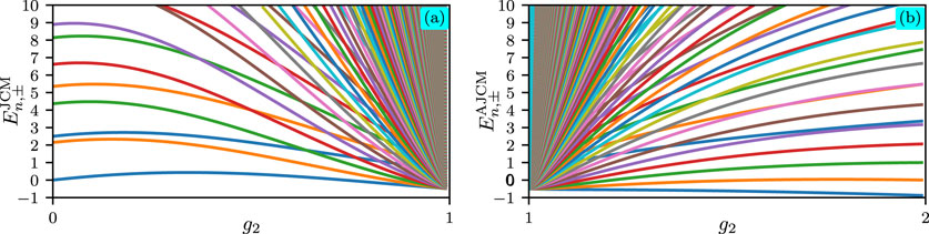
Figure 1. Energy levels of the anisotropic quantum Rabi model for the first ten states $(n,\pm =10)$ are plotted as a function of the coupling parameter $g_2$, with fixed parameters ${\omega }_D=2.5$, ${\omega }_0=1.0$, and $g_1=1.0$. In Panel (a), the eigenvalues correspond to the Jaynes-Cummings regime $(g_2<g_1)$, where the energy levels $E_{n,\pm }^{\text{JCM}}$ are derived from Equation 5. Panel (b) illustrates the eigenvalues for the anti-Jaynes-Cummings regime $(g_2>1)$, with the energy levels $E_{n,\pm }^{\text{AJCM}}$ also determined by Equation 5. This separation highlights the distinct behaviors of the system in the two coupling regimes.

To conclude this section, we present an analysis of the atomic inversion for the anisotropic quantum Rabi model with diamagnetic term in the two distinct coupling regimes. The atomic inversion, denoted as $W(t)$, is a fundamental quantity that characterizes the dynamics of the system. It is defined as the difference in population between the atomic states $|\uparrow \rangle$ and $|\downarrow \rangle$, and is mathematically expressed as: $W(t)=⟨{\widehat{\sigma }}_z(t)⟩$. This quantity provides insight into the temporal evolution of the atomic populations and serves as a key indicator of the system’s behavior under different coupling conditions. In the two parameter regimes under consideration, the atomic inversion is given by: $W(t)=⟨\psi (0)|{\widehat{U}}^{†}(t){\widehat{\sigma }}_z\widehat{U}(t)|\psi (0)⟩$, where $\widehat{U}(t)$ represents the time evolution operator. This operator is defined as: $\widehat{U}(t)=\exp [-i\widehat{H}t]$. Here, $|\psi (0)\rangle$ denotes the initial state of the system, which is the tensor product of the field state and the initial atomic state. The atomic inversion captures the interplay between the atomic and field degrees of freedom, reflecting the influence of the coupling parameters $g_1$ and $g_2$. For each parameter regime, the atomic inversion takes the following form:

$W\left(t\right)=\left\{\begin{array}{cc}⟨\psi \left(0\right)|\widehat{S}\left(r\right){\widehat{U}}_{\text{JCM}}^{†}\left(t\right){\widehat{S}}^{†}\left(r\right){\widehat{\sigma }}_z\widehat{S}\left(r\right){\widehat{U}}_{\text{JCM}}\left(t\right){\widehat{S}}^{†}\left(r\right)|\psi \left(0\right)⟩,\hfill & \text{if\hspace{0.17em}}{g}_2<g_1,\hfill \\ ⟨\psi \left(0\right)|\widehat{S}\left(r\right){\widehat{U}}_{\text{AJCM}}^{†}\left(t\right){\widehat{S}}^{†}\left(r\right){\widehat{\sigma }}_z\widehat{S}\left(r\right){\widehat{U}}_{\text{AJCM}}\left(t\right){\widehat{S}}^{†}\left(r\right)|\psi \left(0\right)⟩,\hfill & \text{if\hspace{0.17em}}{g}_1<g_2.\hfill \end{array}\right.$

The time evolution operator for the anisotropic quantum Rabi model with diamagnetic term is expressed as:

$\widehat{U}\left(t\right)=\left\{\begin{array}{cc}\widehat{S}\left(r\right){\widehat{U}}_{\text{JCM}}\left(t\right){\widehat{S}}^{†}\left(r\right),\hfill & \text{for\hspace{0.17em}}{g}_2<g_1,\hfill \\ \widehat{S}\left(r\right){\widehat{U}}_{\text{AJCM}}\left(t\right){\widehat{S}}^{†}\left(r\right),\hfill & \text{for\hspace{0.17em}}{g}_1<g_2.\hfill \end{array}\right.(6)$

The evolution operators corresponding to the Jaynes-Cummings and anti-Jaynes-Cummings Hamiltonians are given by:

$\begin{array}{ll}\hfill & {\widehat{U}}_{\text{JCM}}=e^{-it{\omega }_{\text{eff}}\left({\widehat{a}}^{†}\widehat{a}+\frac{{\widehat{\sigma }}_z}{2}\right)}\left[\begin{array}{cc}\hfill {\widehat{U}}_{11}^{\text{JCM}}\left(t\right)\hfill & \hfill {\widehat{U}}_{12}^{\text{JCM}}\left(t\right)\hfill \\ \hfill {\widehat{U}}_{21}^{\text{JCM}}\left(t\right)\hfill & \hfill {\widehat{U}}_{22}^{\text{JCM}}\left(t\right)\hfill \end{array}\right],\hfill \\ \hfill & {\widehat{U}}_{\text{AJCM}}=e^{-it{\tilde{\omega }}_{\text{eff}}\left({\widehat{a}}^{†}\widehat{a}-\frac{{\widehat{\sigma }}_z}{2}\right)}\left[\begin{array}{cc}\hfill {\widehat{U}}_{11}^{\text{AJCM}}\left(t\right)\hfill & \hfill {\widehat{U}}_{12}^{\text{AJCM}}\left(t\right)\hfill \\ \hfill {\widehat{U}}_{21}^{\text{AJCM}}\left(t\right)\hfill & \hfill {\widehat{U}}_{22}^{\text{AJCM}}\left(t\right)\hfill \end{array}\right],\hfill \end{array}$

respectively. The matrix elements of the evolution operators are explicitly given by:

$\begin{array}{ll}\hfill & {\widehat{U}}_{11}^{\text{JCM}}\left(t\right)=\cos \left(\frac{{\mathrm{\Omega }}_{\widehat{n}+1}t}{2}\right)-i\frac{{\mathrm{\Delta }}_{\text{eff}}}{{\mathrm{\Omega }}_{\widehat{n}+1}}\sin \left(\frac{{\mathrm{\Omega }}_{\widehat{n}+1}t}{2}\right),\hfill \\ \hfill & {\widehat{U}}_{12}^{\text{JCM}}\left(t\right)=-i2g_{\text{eff}}\frac{\sin \left(\frac{{\mathrm{\Omega }}_{\widehat{n}+1}t}{2}\right)}{{\mathrm{\Omega }}_{\widehat{n}+1}}\widehat{a},\hfill \\ \hfill & {\widehat{U}}_{21}^{\text{JCM}}\left(t\right)=-i2g_{\text{eff}}{\widehat{a}}^{†}\frac{\sin \left(\frac{{\mathrm{\Omega }}_{\widehat{n}+1}t}{2}\right)}{{\mathrm{\Omega }}_{\widehat{n}+1}},\hfill \\ \hfill & {\widehat{U}}_{22}^{\text{JCM}}\left(t\right)=\cos \left(\frac{{\mathrm{\Omega }}_{\widehat{n}}t}{2}\right)+i\frac{{\mathrm{\Delta }}_{\text{eff}}}{{\mathrm{\Omega }}_{\widehat{n}}}\sin \left(\frac{{\mathrm{\Omega }}_{\widehat{n}}t}{2}\right),\hfill \end{array}$

where ${\mathrm{\Delta }}_{\text{eff}}={\omega }_0-{\omega }_{\text{eff}}$, and ${\mathrm{\Omega }}_{\widehat{n}}=\sqrt{{\mathrm{\Delta }}_{\text{eff}}^2+4g_{\text{eff}}^2\widehat{n}}$ (with $\widehat{n}={\widehat{a}}^{†}\widehat{a}$). Similarly, for the anti-Jaynes-Cummings model:

$\begin{array}{ll}\hfill & {\widehat{U}}_{11}^{\text{AJCM}}\left(t\right)=\cos \left(\frac{{\tilde{\mathrm{\Omega }}}_{\widehat{n}}t}{2}\right)-i\frac{{\tilde{\mathrm{\Delta }}}_{\text{eff}}}{{\tilde{\mathrm{\Omega }}}_{\widehat{n}}}\sin \left(\frac{{\tilde{\mathrm{\Omega }}}_{\widehat{n}}t}{2}\right),\hfill \\ \hfill & {\widehat{U}}_{12}^{\text{AJCM}}\left(t\right)=-i2{\tilde{g}}_{\text{eff}}{\widehat{a}}^{†}\frac{\sin \left(\frac{{\tilde{\mathrm{\Omega }}}_{\widehat{n}+1}t}{2}\right)}{{\tilde{\mathrm{\Omega }}}_{\widehat{n}+1}},\hfill \\ \hfill & {\widehat{U}}_{21}^{\text{AJCM}}\left(t\right)=-i2{\tilde{g}}_{\text{eff}}\frac{\sin \left(\frac{{\tilde{\mathrm{\Omega }}}_{\widehat{n}+1}t}{2}\right)}{{\tilde{\mathrm{\Omega }}}_{\widehat{n}+1}}\widehat{a},\hfill \\ \hfill & {\widehat{U}}_{22}^{\text{AJCM}}\left(t\right)=\cos \left(\frac{{\tilde{\mathrm{\Omega }}}_{\widehat{n}+1}t}{2}\right)+i\frac{{\mathrm{\Delta }}_{\text{eff}}}{{\tilde{\mathrm{\Omega }}}_{\widehat{n}+1}}\sin \left(\frac{{\tilde{\mathrm{\Omega }}}_{\widehat{n}+1}t}{2}\right),\hfill \end{array}$

with ${\tilde{\mathrm{\Delta }}}_{eff}={\omega }_0+{\tilde{\omega }}_{eff}$, and ${\tilde{\mathrm{\Omega }}}_{\widehat{n}}=\sqrt{{\tilde{\mathrm{\Delta }}}_{eff}^2+4{\tilde{g}}_{eff}^2\widehat{n}}$.

Figure 2 illustrates the time evolution of the atomic inversion $W(t)$ for the anisotropic quantum Rabi model, including the diamagnetic term, in two distinct coupling regimes: (a) $g_2<g_1$ and (b) $g_1<g_2$. The initial state of the system is chosen as $|\psi (0)\rangle =|\alpha \rangle \otimes |\uparrow \rangle =|\alpha ,\uparrow \rangle$, where $|\alpha \rangle$ represents a coherent state of the field. Therefore, considering the corresponding evolution operator, Equation 6, the atomic inversion is given by

$W\left(t\right)=\left\{\begin{array}{cc}{\displaystyle \sum _{n=0}^{\infty }}|A_n{|}^2\left(\frac{{\mathrm{\Delta }}_{\text{eff}}^2+4g_{\text{eff}}^2\left(n+1\right)\cos \left({\mathrm{\Omega }}_{n+1}t\right)}{{\mathrm{\Delta }}_{\text{eff}}^2+4g_{\text{eff}}^2\left(n+1\right)}\right)\hfill & \text{if\hspace{0.17em}}{g}_2<g_1,\hfill \\ {\displaystyle \sum _{n=0}^{\infty }}|{\tilde{A}}_n{|}^2\left(\frac{{\tilde{\mathrm{\Delta }}}_{\text{eff}}^2+4{\tilde{g}}_{\text{eff}}^{2}n\cos \left({\tilde{\mathrm{\Omega }}}_{n}t\right)}{{\tilde{\mathrm{\Delta }}}_{\text{eff}}^2+4{\tilde{g}}_{\text{eff}}^{2}n}\right)\hfill & \text{if\hspace{0.17em}}{g}_1<g_2,\hfill \end{array}\right.$

where

$\begin{array}{ll}\hfill A_n& =\frac{1}{\sqrt{\cosh \left(r\right)}}\exp \left(-\frac{|{\alpha }_r{|}^2}{2}-\frac{\tanh \left(-r\right)}{2}{\alpha }_r^{*2}\right)\frac{{\tanh }^{n/2}\left(-r\right)}{2^{n/2}\sqrt{n!}}{H}_n\hfill \\ \hfill & \times \left[{\alpha }_r\frac{1+\tanh \left(-r\right)}{\sqrt{2\tanh \left(-r\right)}}\right],\hfill \end{array}$

with ${\alpha }_r=\alpha \cosh (r)+{\alpha }^{*}\sinh (r)$, and $H_n(x)$ being the $n$-th Hermite polynomial. Here, $A_n$ determines the photon probability distribution $|A_n{|}^2$ for $g_2<g_1$, while $|{\tilde{A}}_n{|}^2$, obtained from Equation 4, describes the distribution for $g_1<g_2$, corresponding to the anti-Jaynes-Cummings model. These coefficients arise from the initial coherent state $|\alpha \rangle$ and the squeeze operator ${\widehat{S}}^{†}(r)$, derived from the evolution operator in Equation 6, such that ${\widehat{S}}^{†}(r)\widehat{D}(\alpha )|0\rangle =\widehat{D}({\alpha }_r){\widehat{S}}^{†}(r)|0\rangle$ [25]. The typical revivals of the Jaynes-Cummings model depend on the effective coupling $g_{\text{eff}}=\sqrt{g_1^2-g_2^2}$, reflecting coherent energy exchange between the atom and the field. However, ${\widehat{S}}^{†}(r)$ modifies these dynamics by altering the photon distribution and enhancing or suppressing transitions based on the squeezing parameter $r$. In the anti-Jaynes-Cummings regime $(g_2\gg g_1)$, revivals stabilize, characterized by ${\tilde{g}}_{\text{eff}}=\sqrt{g_2^2-g_1^2}$. As shown in Figure 3, the average photon number and Fock state populations are influenced by $g_2$: higher Fock states populate as $g_2$ approaches $g_1$, while they depopulate for $g_2\gg g_1$. This behavior underscores the role of ${\widehat{S}}^{†}(r)$ in modulating quantum dynamics across both regimes.

Figure 2

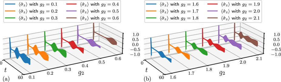
Figure 2. Dynamics of the atomic inversion in the anisotropic quantum Rabi model. The figure illustrates the temporal evolution of the atomic inversion $W(t)$ for two distinct coupling regimes: (a) $g_2<g_1$ and (b) $g_1<g_2$. The initial state of the system is chosen as $|\psi (0)\rangle =|\alpha \rangle \otimes |\uparrow \rangle =|\alpha ,\uparrow \rangle$, where $|\alpha \rangle$ represents a coherent state of the field with $\alpha =3$. Additionally, we have considered different values of $g_2$ for the two distinct parameter regimes with $g_1=1$, and we set $\omega ={\omega }_0=1$.

Figure 3

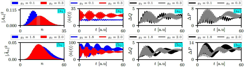
Figure 3. Dynamics of the anisotropic quantum Rabi model in two distinct coupling regimes: (a) Jaynes-Cummings regime $(g_2<g_1)$ and (b) anti-Jaynes-Cummings regime $(g_2>g_1)$, with $g_1=1$ and $\omega ={\omega }_0=1$. The panels show ${\text{a}}_1$, ${\text{b}}_1$ the photon probability distribution $|A_n{|}^2$ or $|{\tilde{A}}_n{|}^2$, ${\text{a}}_2$, ${\text{b}}_2$ the average photon number $⟨\widehat{n}(t)⟩$, ${\text{a}}_3$, ${\text{b}}_3$ the quadrature dispersion $\mathrm{\Delta }Q$, and ${\text{a}}_4$, ${\text{b}}_4$ the quadrature dispersion $\mathrm{\Delta }P$, as functions of time $t$.

Finally, in Figure 3, we show the probability distribution $({\text{a}}_1)$, the average photon number $⟨n(t)⟩$ $({\text{a}}_2)$, and the field quadrature dispersions $\mathrm{\Delta }{Q}^2=⟨x^2(t)⟩-{⟨x(t)⟩}^2$ and $\mathrm{\Delta }{P}^2=⟨p^2(t)⟩-{⟨p(t)⟩}^2$ (${\text{a}}_3$ and ${\text{a}}_4$, respectively; the same is shown for ${\text{b}}_j$): Jaynes-Cummings $g_2=[0.1,0.3]$ and anti-Jaynes-Cummings $g_2=[1.8,2.0]$. The average photon number in the Jaynes-Cummings regime is given by

$\begin{array}{cc}\hfill ⟨\widehat{n}\left(t\right)⟩& =\frac{1}{g_1^2-g_2^2}\left[g_2^2+\left(g_1^2+g_2^2\right){\displaystyle \sum _{n=0}^{\infty }}{\left|A_n\right|}^2\left(n{\left|{\tau }_{n+1}^{\left(11\right)}\right|}^2+{\left(n+1\right)}^2{\left|{\tau }_{n+1}^{\left(21\right)}\right|}^2\right)\right.\hfill \\ \hfill & -2g_1{g}_2\times \hspace{0.17em}{\displaystyle \sum _{n=0}^{\infty }}\sqrt{\left(n+1\right)\left(n+2\right)}\mathrm{R}\mathrm{e}\left\{A_n^{*}{A}_{n+2}{e}^{-i2{\omega }_{eff}t}\left[\left({\tau }_{n+1}^{\left(11\right)*}{\tau }_{n+3}^{\left(11\right)}\right)\right]\right.\hfill \\ \hfill & \left.\left.\left.,+\left(n+3\right){\tau }_{n+1}^{\left(21\right)*}{\tau }_{n+3}^{\left(21\right)}\right]\right\}\right]\hfill \end{array}$

where ${\tau }_n^{(11)}=\cos ({\mathrm{\Omega }}_{n}t/2)-i{\mathrm{\Delta }}_{\text{eff}}\sin ({\mathrm{\Omega }}_{n}t/2)/{\mathrm{\Omega }}_n$, and ${\tau }_n^{(21)}=-i2g_{\text{eff}}\sin ({\mathrm{\Omega }}_{n}t/2)/{\mathrm{\Omega }}_n$. On the other hand, the average photon number in the anti-Jaynes-Cummings regime is

$\begin{array}{cc}\hfill ⟨\widehat{n}\left(t\right)⟩=& \frac{1}{g_2^2-g_1^2}\left[g_1^2+\left(g_1^2+g_2^2\right){\displaystyle \sum _{n=0}^{\infty }}{\left|{\tilde{A}}_{n+1}\right|}^2\left(\left(n+1\right){\left|{\tilde{\tau }}_{n+1}^{\left(11\right)}\right|}^2+n\left(n+1\right){\left|{\tilde{\tau }}_{n+1}^{\left(21\right)}\right|}^2\right)\right]\hfill \\ \hfill & -2g_1{g}_2{\displaystyle \sum _{n=0}^{\infty }}\mathrm{R}\mathrm{e}\left\{{\tilde{A}}_n^{*}{\tilde{A}}_{n+2}\sqrt{\left(n+1\right)\left(n+2\right)}{e}^{-i2{\tilde{\omega }}_{\text{eff}}t}{\tilde{\tau }}_n^{\left(11\right)*}{\tilde{\tau }}_{n+2}^{\left(11\right)}\right.\hfill \\ \hfill & \left.+ {\tilde{A}}_{n+1}^{*}{\tilde{A}}_{n+3}\left(n+1\right)\sqrt{\left(n+2\right)\left(n+3\right)}{e}^{-i2{\tilde{\omega }}_{\text{eff}}t}{\tilde{\tau }}_{n+1}^{\left(21\right)*}{\tilde{\tau }}_{n+3}^{\left(21\right)}\right\}\hfill \end{array}$

where ${\tilde{\tau }}_n^{(11)}=\cos ({\tilde{\mathrm{\Omega }}}_{n}t/2)-i{\tilde{\mathrm{\Delta }}}_{\text{eff}}\sin ({\tilde{\mathrm{\Omega }}}_{n}t/2){\tilde{\mathrm{\Omega }}}_n$, and ${\tilde{\tau }}_n^{(21)}=-i2{\tilde{g}}_{\text{eff}}\sin ({\tilde{\mathrm{\Omega }}}_{n}t/2){\tilde{\mathrm{\Omega }}}_n$. The squeeze operator ${\widehat{S}}^{†}(r)$ fundamentally modifies both the average photon number $⟨\widehat{n}(t)⟩$ and quadrature dispersions $\mathrm{\Delta }Q$, $\mathrm{\Delta }P$ in Jaynes-Cummings $(g_2<g_1)$ and anti-Jaynes-Cummings $(g_1<g_2)$ regimes. Its action transforms photon operators as ${\widehat{S}}^{†}(r){\widehat{a}}^{†}\widehat{a}\widehat{S}(r)={\mu }^2{\widehat{a}}^{†}\widehat{a}-\mu \nu ({\widehat{a}}^2+{\widehat{a}}^{†2})+{\nu }^2\widehat{a}{\widehat{a}}^{†}$, demonstrating how it enhances/suppresses fluctuations via parameter $r$. When applied to a coherent state initial condition $|\alpha \rangle$, it generates a squeezed coherent state $|{\alpha }_r,-r\rangle ={\widehat{S}}^{†}(r)|\alpha \rangle$, whose photon statistics and quadrature properties are distinctly modified compared to the unsqueezed case, with ${\alpha }_r=\alpha \cosh r+{\alpha }^{*}\sinh r$ characterizing the displaced squeezed state. These results demonstrate the operator’s role in controlling quantum dynamics in each regime.

4 Conclusion

It has been demonstrated that, by judiciously tuning the diamagnetic amplitude, the anisotropic quantum Rabi model can be reduced to either the Jaynes-Cummings model or the anti-Jaynes-Cummings model through the application of a squeezing transformation. Specifically, when the condition $\frac{\mu }{\nu }=\frac{g_1}{g_2}$ or $\frac{\mu }{\nu }=\frac{g_2}{g_1}$ is satisfied, where $\mu =\cosh (r)$ and $\nu =\sinh (r)$ are the hyperbolic functions associated with the squeezing parameter $r$, the Hamiltonian of the anisotropic quantum Rabi model transforms into the Jaynes-Cummings Hamiltonian for $g_2<g_1$ or the anti-Jaynes-Cummings Hamiltonian for $g_1<g_2$. In the case of the standard quantum Rabi model (i.e., when $g_1=g_2$), the system cannot be reduced to either the Jaynes-Cummings or anti-Jaynes-Cummings models. However, the squeezing transformation still allows us to eliminate the diamagnetic term, thereby removing the $A^2$ interaction from the Hamiltonian. This result highlights the versatility of the squeezing transformation in simplifying the anisotropic quantum Rabi model and its connection to well-known models in quantum optics.

Data availability statement

The original contributions presented in the study are included in the article/supplementary material, further inquiries can be directed to the corresponding author.

Author contributions

JA-C: Investigation, Methodology, Validation, Writing – original draft, Writing – review and editing. IR-P: Conceptualization, Investigation, Methodology, Software, Writing – original draft, Writing – review and editing. AZ-S: Investigation, Methodology, Supervision, Validation, Writing – original draft, Writing – review and editing. HM-C: Conceptualization, Investigation, Supervision, Writing – original draft, Writing – review and editing.

Funding

The author(s) declare that no financial support was received for the research and/or publication of this article.

Conflict of interest

The authors declare that the research was conducted in the absence of any commercial or financial relationships that could be construed as a potential conflict of interest.

Generative AI statement

The author(s) declare that no Generative AI was used in the creation of this manuscript.

Publisher’s note

All claims expressed in this article are solely those of the authors and do not necessarily represent those of their affiliated organizations, or those of the publisher, the editors and the reviewers. Any product that may be evaluated in this article, or claim that may be made by its manufacturer, is not guaranteed or endorsed by the publisher.

References

1. Jaynes ET, Cummings FW. Comparison of quantum and semiclassical radiation theories with application to the beam maser. Proc IEEE (1963) 51:89–109. doi:10.1109/PROC.1963.1664

CrossRef Full Text | Google Scholar

2. Gerry CC, Knight PL. Introductory quantum optics. Cambridge, Cambridge University Press (2004). doi:10.1017/CBO9780511791239

CrossRef Full Text | Google Scholar

3. Larson J, Mavrogordatos TK. The jaynes–cummings model and its descendants. China, Institute of Physics Publishing (2022).

Google Scholar

4. Meher N, Sivakumar S. A review on quantum information processing in cavities. Eur Phys J Plus (2022) 137:985. doi:10.1140/epjp/s13360-022-03172-x

CrossRef Full Text | Google Scholar

5. Meher N, Sivakumar S. Number state filtered coherent states. Quan Inf. Process. (2018) 17:233. doi:10.1007/s11128-018-1995-6

CrossRef Full Text | Google Scholar

6. Meher N, Sivakumar S, Panigrahi PK. Duality and quantum state engineering in cavity arrays. Sci Rep (2017) 7:9251. doi:10.1038/s41598-017-08569-8

PubMed Abstract | CrossRef Full Text | Google Scholar

7. Crisp MD. Interaction of a charged harmonic oscillator with a single quantized electromagnetic field mode. Phys Rev A (1991) 44:563–73. doi:10.1103/PhysRevA.44.563

PubMed Abstract | CrossRef Full Text | Google Scholar

8. Crisp MD. Jaynes’ steak dinner problem II. Cambridge, Cambridge University Press (1993). p. 81–90. doi:10.1017/CBO9780511524448

CrossRef Full Text | Google Scholar

9. Kockum AF, Miranowicz A, Liberato SD, Savasta S, Nori F. Ultrastrong coupling between light and matter. Nat Rev Phys (2019) 1:19–40. doi:10.1038/s42254-018-0006-2

CrossRef Full Text | Google Scholar

10. Salado-Mejía M, Román-Ancheyta R, Soto-Eguibar F, Moya-Cessa HM. Spectroscopy and critical quantum thermometry in the ultrastrong coupling regime. Quan Sci Technology (2021) 6:025010. doi:10.1088/2058-9565/abdca5

CrossRef Full Text | Google Scholar

11. Qin W, Kockum F, Sanchez Muñoz C, Miranowicz A, Nori F. Quantum amplification and simulation of strong and ultrastrong coupling of light and matter. Phys Rep (2024) 1078:1–59. doi:10.1016/j.physrep.2024.05.003

CrossRef Full Text | Google Scholar

12. Moya-cessa H, Roversi JA, Dutra SM, Vidiella-barranco A. Recovering coherence from decoherence: a method of quantum-state reconstruction. Phys Rev A (1999) 60:4029–33. doi:10.1103/PhysRevA.60.4029

CrossRef Full Text | Google Scholar

13. Rabi II. Space quantization in a gyrating magnetic field. Phys Rev (1937) 51:652–4. doi:10.1103/PhysRev.51.652

CrossRef Full Text | Google Scholar

14. Swain S. Continued fraction expressions for the eigensolutions of the Hamiltonian describing the interaction between a single atom and a single field mode: comparisons with the rotating wave solutions. J Phys A (1973) 6:1919–34. doi:10.1088/0305-4470/6/12/016

CrossRef Full Text | Google Scholar

15. Moya-Cessa H, Vidiella-Barranco A, Roversi J, Dutra S. Unitary transformation approach for the trapped ion dynamics. J Opt B: Quan Semiclass. Opt. (2000) 2:21–3. doi:10.1088/1464-4266/2/1/303

CrossRef Full Text | Google Scholar

16. Chen Q-H, Liu T, Zhang Y-Y, Wang K-L. Exact solutions to the Jaynes-Cummings model without the rotating-wave approximation. EPL (2011) 96:14003. doi:10.1209/0295-5075/96/14003

CrossRef Full Text | Google Scholar

17. Braak D. Integrability of the Rabi model. Phys Rev Lett (2011) 107:100401. doi:10.1103/PhysRevLett.107.100401

PubMed Abstract | CrossRef Full Text | Google Scholar

18. Xie Q-T, Cui S, Cao J-P, Amico L, Fan H. Anisotropic Rabi model. Phys Rev X (2014) 4:021046. doi:10.1103/PhysRevX.4.021046

CrossRef Full Text | Google Scholar

19. Ye T, Wang C, Chen Q-H. Anisotropic qubit-photon interactions inducing multiple antibunching-to-bunching transitions of photons. Opt Express (2024) 32:33483–93. doi:10.1364/OE.533310

PubMed Abstract | CrossRef Full Text | Google Scholar

20. Boutakka Z, Sakhi Z, Bennai M. Quantum entanglement in the Rabi model with the presence of the A² term. Int J Theor Phys (2024) 63:274. doi:10.1007/s10773-024-05805-6

CrossRef Full Text | Google Scholar

21. Satyanarayana MV, Rice P, Vyas R, Carmichael HJ. Ringing revivals in the interaction of a two-level atom with squeezed light. J Opt Soc Am B (1989) 6:228–37. doi:10.1364/JOSAB.6.000228

CrossRef Full Text | Google Scholar

22. Rodriguez-Lara BM, Moya-Cessa H, Klimov AB. Combining Jaynes-Cummings and anti-Jaynes-Cummings dynamics in a trapped-ion system driven by a laser. Phys Rev A (2005) 71:023811. doi:10.1103/PhysRevA.71.023811

CrossRef Full Text | Google Scholar

23. Bocanegra-Garay IA, Castillo-Celeita M, Negro J, Nieto L, Gómez-Ruiz FJ. Exploring supersymmetry: interchangeability between Jaynes-Cummings and anti-Jaynes-Cummings models. Phys Rev Res (2024) 6:043218. doi:10.1103/PhysRevResearch.6.043218

CrossRef Full Text | Google Scholar

24. Zúñiga-Segundo A, Rodríguez-Lara BM, Fernández CDJ, Moya-Cessa HM. Jacobi photonic lattices and their susy partners. Opt Express (2014) 22:987–94. doi:10.1364/OE.22.000987

PubMed Abstract | CrossRef Full Text | Google Scholar

25. Hernández-Sánchez L, Ramos-Prieto I, Soto-Eguibar F, Moya-Cessa HM. Effects of squeezing on the power broadening and shifts of micromaser lineshapes. Photonics (2024) 11:371. doi:10.3390/photonics11040371

CrossRef Full Text | Google Scholar