Calculation of radiative thickness using spherical harmonic methods for the radiative transfer equation

The radiative transfer equation (RTE) plays a fundamental role in modeling photon transport in various media such as biological tissues and atmospheric systems, where scattering phenomena are critical. In this study, the RTE is solved using two spherical harmonic-based numerical techniques: the Chebyshev and Legendre polynomial methods. Both the Henyey–Greenstein (HG) and Anlı–Güngör (AG) scattering phase functions are employed to analyze their effectiveness in radiative thickness computations. The Marshak boundary condition is applied, and the eigenvalue problems are solved using Mathematica software across various single scattering albedo values (ω) and anisotropy coefficients (g). The results indicate that the AG phase function produces outcomes highly consistent with the HG function, demonstrating numerical robustness and stability for both methods. These findings suggest that the AG phase function, commonly used in neutron transport, can be effectively applied in radiative transfer modeling as a computationally efficient and accurate alternative in biomedical and atmospheric applications.

1 Introduction

The radiative transfer theory has been employed to describe the random transfer of energy through a medium occupied by active radiation in many disciplines, including nuclear reactor physics, astrophysics, atmospheric physics, remote sensing, and biological tissue optics [1–7]. The general problem addressed by the radiative transfer theory is the availability of some particular physical quantity: the radiant intensity, the radiant energy density vector, or the radiant energy density vector flux that depends on the location, the direction, and the frequency of the active radiation [8]. It is also applicable to many engineering areas [9–13].

The radiative transfer equation (RTE) is an integro-differential equation that governs the behavior of the radiant heat flux in turbulent media, which includes gases, aerosols, and biological tissues as particular examples [14]. The RTE plays a crucial role in the thermal design of systems; it represents the main mechanism for the dissipation of thermal energy [15]. The solution of the RTE is essential for the sizing of primary and secondary loads. Parameter estimation of biological tissues in the diagnostic or therapeutic assessments also requires the solution of the RTE and is extremely important in oncology for tumor localization and thermal therapy [16].

The RTE is solved using analytical and numerical methods [17–20]. The radiative transfer equation solution can be done for reflectivity, transmissivity, albedo, or optical thickness [21–24]. Although the RTE has been solved by a variety of methods, those based on spherical harmonics are employed most frequently [24–27]. In the radiative system, the transportation of a photon through media becomes anisotropic. It is therefore necessary to take into consideration the anisotropic scattering case in the context of one-dimensional slab geometries. The Henyey–Greenstein (HG) phase function is widely used in radiative transfer modeling to describe the angular distribution of scattered light in a medium [28, 29]. While the HG phase function is widely used in radiative transfer calculations, its formulation includes a (2n+1) multiplier, which significantly increases computational effort for higher-order iterations.

Motivated by the structural similarities between the Anlı–Güngör (AG) and the HG phase functions, this study examines the applicability of the AG function within the framework of the RTE. The AG scattering function is a phase function that is frequently employed in the solution of neutron transport equations [30]. The observation that both functions possess analogous structures has given rise to a question regarding the applicability of the AG phase function to the RTE in a manner analogous to that of the HG function. To assess its applicability, radiative thickness solutions were conducted through two distinct methodologies: the Legendre and Chebyshev polynomial methods. By employing the Chebyshev method to determine optical thickness and validating the results against the Legendre polynomial method, we assess the accuracy and computational efficiency of these phase functions in radiative transfer. Mathematica software was implemented on a high-speed digital computer to structure the obtained algorithm. The Marshak boundary condition was applied to calculate the thickness. The calculations were performed with single scattering albedo numbers greater than one, in steps of 0.2. The anisotropy coefficient g corresponding to each single scattering albedo number was calculated in steps of 0.1 from 0.1 to 0.9. The solution set of the equation was analyzed in detail. The ensuing results are presented in tabular and graphical formats. The compatibility of the results from the two scattering functions was established. This comparison provides new insights into whether alternative phase functions can be effectively used in radiative transport modeling, offering a computational advantage without compromising accuracy. The findings of this study contribute to the ongoing efforts to refine radiative transfer models for various scientific and engineering applications.

2 Solution methods of the radiative transfer equation

2.1 Chebyshev solution method

The radiative transfer equation is a fundamental equation in the field of radiation physics, which provides a theoretical framework for the calculation of the photon distribution in a scattering, emitting, and absorbing medium. Consequently, the model incorporates multiple unknown parameters, which are associated with the characteristics of the medium and the intricacy of the geometric configuration. To render the equation more solvable, certain assumptions must be made. The time-independent, monoenergetic RTE in plane geometry for the unpolarized case can be expressed as [31]:

$\mu \frac{d}{dx}I\left(x,\mu \right)+I\left(x,\mu \right)=\frac{\omega }{2}{\displaystyle \underset{-1}{\overset{1}{\int }}}f\left(\mu ,{\mu }^{\prime }\right)I\left(x,\mu \right)d{\mu }^{\prime ,}(1)$

where $I\left(x,\mu \right)$ is known as the angular intensity, $f\left(\mu ,{\mu }^{\prime }\right)$ defines the phase function, x is the optical variable, $\mu$ is the cosine angle between the propagation direction and the positive x-axis, and ω is the single scattering albedo ratio of the scattering coefficient to the extinction coefficient.

The scattering phase function is defined for the HG [32].

$f\left(\mu ,{\mu }^{\prime }\right)={\displaystyle \sum _{n=0}^N}\left(2n+1\right)g^n{P}_n\left(\mu \right)P_n\left({\mu }^{\prime }\right).(2)$

For the Anlı-Güngör scattering function,

$f\left(\mu ,{\mu }^{\prime }\right)={\displaystyle \sum _{n=0}^N}{g}^n{P}_n\left(\mu \right)P_n\left({\mu }^{\prime }\right).(3)$

In Equations 2, 3, $g^n$ is the scattering coefficient, −1 < g < 1. In the visible spectrum, the anisotropy parameter of $g$ in biological tissues ranges from 0.65 to 0.95 [33]. So, in this study, the g parameter is taken into consideration from 0 to 1 to consider a wide range of possibilities. $P_n\left(\mu \right)$ is the Legendre polynomial.

The angular intensity function of the RTE is expanded in terms of Chebyshev polynomials:

$I\left(x,\mu \right)=\frac{{\varphi }_0\left(x\right)T_0\left(\mu \right)}{\pi \sqrt{1-{\mu }^2}}+\frac{2}{\pi }{\displaystyle \sum _{n=1}^N}\frac{{\varphi }_n\left(x\right)T_n\left(\mu \right)}{\sqrt{1-{\mu }^2}}.(4)$

The HG and AG scatterings are substituted into the radiative transfer equation in Equation 1, respectively:

$\mu \frac{d}{dx}I\left(x,\mu \right)+I\left(x,\mu \right)=\frac{\omega }{2}{\displaystyle \sum _{n=0}^N}\left(2n+1\right)g^n{P}_n\left(\mu \right){\displaystyle \underset{-1}{\overset{1}{\int }}}{T}_n\left({\mu }^{\prime }\right)I\left(x,\mu \right)d{\mu }^{\prime ,}(5)$

$\mu \frac{d}{dx}I\left(x,\mu \right)+I\left(x,\mu \right)=\frac{\omega }{2}{\displaystyle \sum _{n=0}^N}{g}^n{P}_n\left(\mu \right){\displaystyle \underset{-1}{\overset{1}{\int }}}{T}_n\left({\mu }^{\prime }\right)I\left(x,\mu \right)d{\mu }^{\prime .}(6)$

Equation 4 is substituted into the general form of the RTE as in Equation 1 with the scattering function in Equation 5 and Equation 6, respectively. The resultant equation occurs after substituting the HG scattering function and Chebyshev expansion for the angular flux, which has been solved by using the recurrence and the orthogonality relations. Then, the mth order Chebyshev polynomial $T_m\left(\mu \right)$ is applied and integrated over [−1, 1] to both sides of the equation to determine the infinite set of ordinary differential equations as follows:

$\frac{d{\varphi }_1\left(x\right)}{dx}+{\varphi }_0\left(x\right)=\omega {\varphi }_0\left(x\right)(\mathrm{7a})$

$\frac{d{\varphi }_2\left(x\right)}{dx}+\frac{d{\varphi }_0\left(x\right)}{dx}+2{\varphi }_1\left(x\right)=2\omega g{\varphi }_1\left(x\right)(\mathrm{7b})$

$\frac{d{\varphi }_3\left(x\right)}{dx}+\frac{d{\varphi }_1\left(x\right)}{dx}+2{\varphi }_2\left(x\right)=-2\omega \left(\frac{1}{3}\left(1-g^2\right){\varphi }_0\left(x\right)-g^2{\varphi }_2\left(x\right)\right).(\mathrm{7c})$

The differential sets for Hg result are shown in Equations 7a–7c. The same procedure is applied for the AG function. The recurrence and the orthogonality relations are used, and then, $T_m\left(\mu \right)$ is multiplied and integrated over [−1, 1] to obtain the differential sets as

$\frac{d{\varphi }_1\left(x\right)}{dx}+{\varphi }_0\left(x\right)=\omega {\varphi }_0\left(x\right)(\mathrm{8a})$

$\frac{d{\varphi }_2\left(x\right)}{dx}+\frac{d{\varphi }_0\left(x\right)}{dx}+2{\varphi }_1\left(x\right)=2\omega \left(\frac{g}{3}\right){\varphi }_1\left(x\right)(\mathrm{8b})$

$\frac{d{\varphi }_3\left(x\right)}{dx}+\frac{d{\varphi }_1\left(x\right)}{dx}+2{\varphi }_2\left(x\right)=-2\omega \left(\frac{1}{15}\left(5-g^2\right){\varphi }_0\left(x\right)-\frac{g^2}{5}{\varphi }_2\left(x\right)\right).(\mathrm{8c})$

The differential sets in Equations 8a–8c are solved by using the proposal as

${\varphi }_n\left(x\right)=A_n\left(\nu \right)e^{x/v}(9)$

The eigen-spectrum of the radiative transfer equation for the HG phase function is obtained in Equations 10a–10c as,

$A_1\left(\nu \right)+v{A}_0\left(\nu \right)=w{A}_0\left(\nu \right)(\mathrm{10a})$

$A_2\left(\nu \right)+A_0\left(\nu \right)+2v{A}_1\left(\nu \right)=2vw{gA}_1\left(\nu \right)(\mathrm{10b})$

$A_3\left(\nu \right)+A_1\left(\nu \right)+2v{A}_2\left(\nu \right)=-2vw\left(\frac{1}{3}\left(1-g^2\right)A_0\left(v\right)-g^2{A}_2\left(v\right)\right).(\mathrm{10c})$

The eigen-spectrum of the radiative transfer equation for the AG phase function is obtained in Equations 11a–11c as

$A_1\left(\nu \right)+v{A}_0\left(\nu \right)=w{A}_0\left(\nu \right)(\mathrm{11a})$

$A_2\left(\nu \right)+A_0\left(\nu \right)+2v{A}_1\left(\nu \right)=2vw{\left(\frac{g}{3}\right)A}_1\left(\nu \right)(\mathrm{11b})$

$A_3\left(\nu \right)+A_1\left(\nu \right)+2v{A}_2\left(\nu \right)=-2vw\left(\frac{1}{15}\left(5-g^2\right)A_0\left(v\right)-\frac{g^2}{5}{A}_2\left(v\right)\right).(\mathrm{11c})$

The eigenvalues $\nu$ can be calculated with dependency on g and $w$ values. The eigenvalues for the solution of the HG and AG phase functions of the RTE have a crucial role. For each situation, the eigenvalues are calculated one by one. The discrete eigenvalues of the RTE for Chebyshev polynomial solutions are determined by solving these ordinary differential equations (ODEs) numerically using Mathematica.

2.2 Legendre polynomial method solution

The RTE solution is done by using the Legendre polynomial method for inverse solution [34], the spherical medium with the P_N method [35], and Green’s method [36, 37]. The powerful ability of the Legendre to solve the RTE based on an integro-differential equation is used for the present study. That is also assumed to be the exact result of the method. The Chebyshev and the Legendre polynomial methods come from the spherical harmonics family, and the solution steps are similar to each other. First, introduce the angular intensity in terms of the Legendre polynomial as

$I\left(x,\mu \right)=\frac{1}{2}{\displaystyle \sum _{n=0}^N}\left(2n+1\right)P_n\left(\mu \right){\varphi }_n\left(x\right).(12)$

Equation 12 and the phase function for HG in Equation 2 are substituted into Equation 1:

$\mu \frac{d}{dx}I\left(x,\mu \right)+I\left(x,\mu \right)=\frac{\omega }{2}{\displaystyle \sum _{n=0}^N}\left(2n+1\right)g^n{P}_n\left(\mu \right){\displaystyle \underset{-1}{\overset{1}{\int }}}{P}_n\left({\mu }^{\prime }\right)I\left(x,\mu \right)d{\mu }^{\prime }.(13)$

The recursion and the orthogonality relations are applied, and the resulting equation is multiplied by $P_m\left(\mu \right)$ and integrated over $\mu \in \left[-1,1\right]$ and the obtained result is shown in Equation 13. It can be found the differential sets after the algebra as shown in Equations 14a–14c,

$\frac{d{\varphi }_1\left(x\right)}{dx}+{\varphi }_0\left(x\right)=\omega {\varphi }_0\left(x\right)(\mathrm{14a})$

$2\frac{d{\varphi }_2\left(x\right)}{dx}+\frac{d{\varphi }_0\left(x\right)}{dx}+3{\varphi }_1\left(x\right)=3\omega g{\varphi }_1\left(x\right)(\mathrm{14b})$

$3\frac{d{\varphi }_3\left(x\right)}{dx}+2\frac{d{\varphi }_1\left(x\right)}{dx}+5{\varphi }_2\left(x\right)=\omega \left(5g^2{\varphi }_2\left(x\right)\right).(\mathrm{14c})$

The general form is written as

$\left(n+1\right)\frac{d{\varphi }_{n+1}\left(x\right)}{dx}+n\frac{d{\varphi }_{n-1}\left(x\right)}{dx}+\left(2n+1\right){\varphi }_n\left(x\right)=\omega \left(2n+1\right)g^n{\varphi }_n\left(x\right)(15)$

The same proposed eigenfunction used in Equation 9 is used to find the eigenvalues. The analytical solution found by applying Equation 9 to Equation 15:

$\left(n+1\right)A_{n+1}\left(v\right)+n{A}_{n-1}\left(v\right)+\left(2n+1\right)v{A}_n\left(v\right)=v\omega \left(2n+1\right)g^n{A}_n\left(v\right)(16)$

So, the general expression is shown in Equation 16. The second phase function AG is used to find the solution of the RTE. The phase function in Equation 3 and the angular intensity in Equation 12 are substituted into the general form in Equation 1:

$\mu \frac{d}{dx}I\left(x,\mu \right)+I\left(x,\mu \right)=\frac{\omega }{2}{\displaystyle \sum _{n=0}^N}{g}^n{P}_n\left(\mu \right){\displaystyle \underset{-1}{\overset{1}{\int }}}{P}_n\left({\mu }^{\prime }\right)I\left(x,\mu \right)d{\mu }^{\prime }(17)$

The resulting equation is displayed in Equation 17. After multiplying with $P_m\left(\mu \right)$ and integrating over $\mu \in \left[-1,1\right]$ using recursion and orthogonality, it is found as

$\left(n+1\right)\frac{d{\varphi }_{n+1}\left(x\right)}{dx}+n\frac{d{\varphi }_{n-1}\left(x\right)}{dx}+\left(2n+1\right){\varphi }_n\left(x\right)=\omega g^n{\varphi }_n\left(x\right)(18)$

The Equation 18 is the general form of the angular moments. After applying the same proposal and making the algebraic calculations, one can find that

$\left(n+1\right)A_{n+1}\left(v\right)+n{A}_{n-1}\left(v\right)+\left(2n+1\right)v{A}_n\left(v\right)=v\omega g^n{A}_n\left(v\right).(19)$

The solution of the resulting equation is shown in Equation 19 gives us the discrete eigenvalues of the problem. In the present study, it is used for the thickness after applying the boundary conditions.

The angular moment ${\varphi }_n\left(x\right)$ can be written by using the discrete eigenvalues for an odd number of N. The angular moment is substituted into angular intensity for each method and the resultant angular intensity is obtained in Equation 20:

${\varphi }_n\left(x\right)={\displaystyle \sum _{n=0}^N}{\displaystyle \sum _{m=1}^{\frac{N+1}{2}}}{B}_k{A}_n\left(v_m\right)\left[e^{x/v_m}+{\left(-1\right)}^n{e}^{-x/v_m}\right],n,m=1,2,3,...,N(20)$

Here, the parity rule is applied to the eigenfunction as $A_n\left(-v\right)={\left(-1\right)}^n{A}_n\left(v\right)$. The coefficient $B_k$ is found from the applied boundary condition. The root of the eigenfunctions gives the eigenvalues for a certain iteration. The spectrum of the roots is modified with the value of the single scattering albedo numbers. The eigenvalues are real for ɷ <1, and real and complex roots are found for ɷ >1 values. The discrete eigenvalues play a crucial role in the solution of the radiative thickness. The angular flux obtained depends on the angular moments, and it also includes the discrete eigenvalues. The eigenvalues are obtained for each iteration separately. The all-solution methods have eigenvalues that depend on the iteration number. In this study, all results are obtained for the N = 7 iteration number. It means that there are (N+1)/2 eigenvalues. That is, four eigenvalues are obtained from the solution method of the eigenfunctions. The eigenfunction is defined for the Chebyshev polynomial method in Equation 11a and for the Legendre polynomial in Equation 19. For example, if one wants to find the P₇ result of the radiative thickness, first, the A_N+1(v) = 0 (P8 = 0) must be used, and four different eigenvalues are obtained from the solution of the eigenfunction. Then the angular flux is expanded to eight, and the eigenvalues are substituted into the equation. As a result, (N+1)/2 x (N+1)/2 square matrices are found. The radiative thickness is the solution of the resultant equation after taking the determinant of the matrices and finding the root for the fixed w and g values. The same process is applied for each different w and g value, and the radiative thicknesses are obtained from the solution of the matrices. For this reason, the angular flux $I\left(x,\mu \right)$ has discrete values for the radiative thickness. The structure of the equation obtained after applying the Chebyshev and Legendre polynomial methods does not permit drawing a graph of angular flux versus thickness.

2.3 Application of the boundary condition

In the study, the solution of the RTE is done for a plane geometrical system. Photons in a homogeneous medium travel up to a certain distance. The distance can be found by using some boundary conditions. Here, the Marshak boundary condition is applied to find the maximum distance that can be reached by photons [38]. The Marshak boundary condition implies zero incoming angular flux on the boundaries. This condition incorporates the reflection of photons accurately using Fresnel’s equations [39–41]. Marshak-type boundary conditions provide a robust way to handle complex radiative transfer problems by accurately modeling the interaction between radiation and the boundaries of a medium. The radiation field is also initialized, often to zero or a steady-state value consistent with no prior radiation flux.

The Marshak boundary condition is defined as

$\underset{\mathbf{0}}{\overset{\mathbf{1}}{\int }}{P}_k\left(-\mu \right)I\left(\tau ,-\mu \right)d\mu =0,k=1,3,5,...,N(21)$

Equation 21 is defined for the P_N method. Here, $\tau$ is the radiative thickness.

$\underset{\mathbf{0}}{\overset{\mathbf{1}}{\int }}{T}_k\left(-\mu \right)I\left(\tau ,-\mu \right)d\mu =0,k=1,3,5,...,N(22)$

Equation 22 is defined for the T_N method. The radiative thicknesses are found by applying the Marshak boundary condition for each method separately.

3 Results and discussion

This work used the P₇ and T₇ techniques for the HG and AG scattering phase functions to compute essential slab thicknesses for radiative transfer systems. The outcomes reveal that the two approaches are reliable in solving the RTE, with a high degree of consistency between them. Additionally, by comparing the HG and AG phase functions, the AG phase function is shown to be a good substitute for RTE solutions, expanding on its well-established use in neutron transport equations (NTE).

According to the study’s findings, the AG scattering phase function, which has traditionally been used for NTE, may now be applied to radiative transfer applications. This crossover demonstrates the AG phase function’s versatility and suggests that it may find broader applications in atmospheric radiative transfer, remote sensing, and biomedical optics.

The seventh iteration of the approaches' solutions is completed. The values of the single scattering albedo are considered for $\omega$ = 1.2, 1.4, 1.6, 1.8, and 2.0. The solutions produced benchmark outcomes throughout a broad spectrum. The anisotropy parameter is significant in biological tissue or air transport. The anisotropy parameter g is commonly used to describe forward scattering, which is particularly relevant in atmospheric and biomedical optics. For highly forward-scattering media, g approaches one (e.g., in biological tissues or clouds). The computational processes are done by using the Mathematica code.

The radiative thickness results are obtained by employing the discrete eigenvalues that are computed from the two distinct applied methods. The all-thickness values are obtained successively, contingent on the varying anisotropy parameter g and single scattering parameter ω. For the seventh iteration of the methods, the derived four eigenvalues are substituted into the applied boundary condition in Equation 21 for the Legendre method and in Equation 22 for the Chebyshev method. The all-computed eigenvalues are tabulated in Table 1. To calculate radiative thickness, refer to the values in Table 1. According to Table 1, in the context of the HG phase function, the eigenvalues obtained through the TN method are, in general, higher than those computed with the PN method, particularly for higher anisotropy values (i.e., larger g). This discrepancy becomes particularly evident for high single scattering albedo values (ω ≥ 1.6), where the influence of directional scattering is more pronounced. Conversely, the AG phase function consistently yields smoother and more regular eigenvalue progressions for both the PN and TN methods. The discrepancy between the PN and TN methods is significantly reduced under the AG function, indicating its numerical robustness and stability.

Table 1

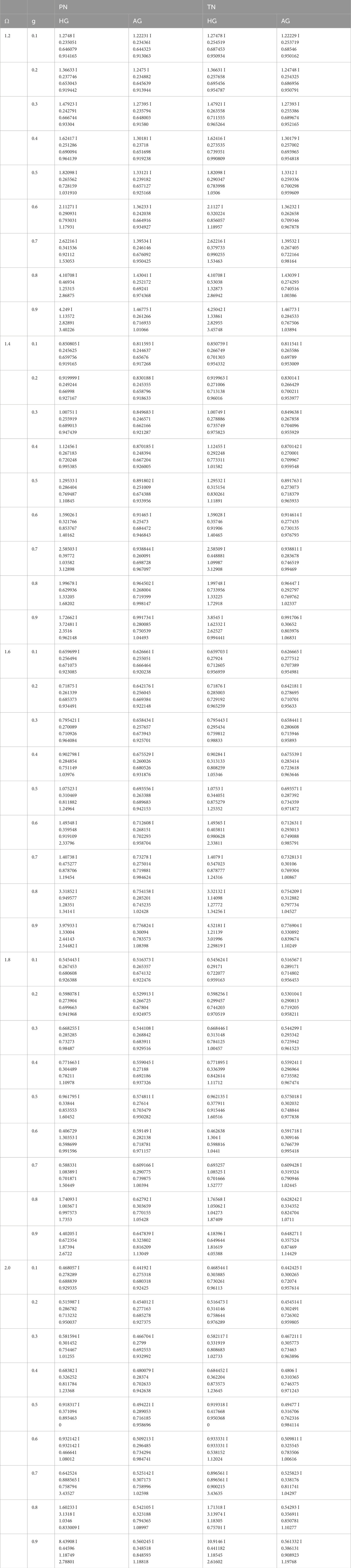
Table 1. Discrete eigenvalues of the PN and TN methods for HG and AG phase functions.

The selected third root from four discrete eigenvalues is demonstrated with graphs in Figure 1. The behavior of the eigenvalues can be shown from the graph. The third eigenvalues obtained using the PN method for the Henyey–Greenstein (HG) phase function exhibit a generally increasing trend concerning the anisotropy parameter g. For ω = 1.4 and ω = 2.0, the eigenvalue curves show abrupt increases at higher g values. At lower g values, the eigenvalues are closely clustered, reflecting stability in weakly anisotropic scattering conditions. The AG phase function under the PN method shows a smooth and monotonic increase for all values of ω. No abrupt changes or spikes are observed in any curve. This behavior confirms the numerical robustness of the AG phase function and its ability to represent scattering effects in a stable and controlled manner. When the HG phase function is applied within the TN method, the resulting third eigenvalues tend to be higher and more oscillatory than those obtained with the PN method. Particularly for ω = 1.4 and ω = 2.0, the eigenvalue curves display sudden changes and irregular behavior at higher g values. The combination of the AG phase function with the TN method yields the most stable and consistent results among all tested configurations. For every ω value, the third eigenvalues increase gradually with increasing g, and no abrupt transitions or numerical instabilities are detected. These results demonstrate that the AG phase function ensures robust numerical performance and consistent physical outcomes when applied with both the PN and the TN schemes.

Figure 1

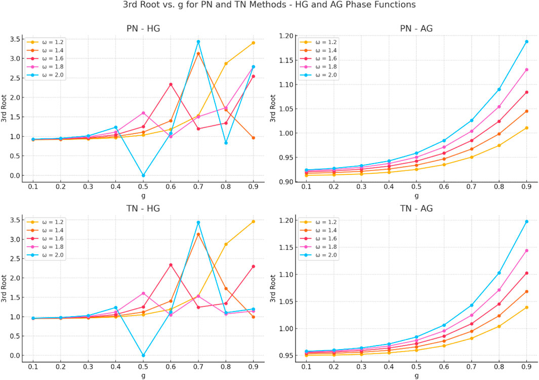
Figure 1. Discrete eigenvalues vs. g graphs for the HG and AG phase functions with the PN and TN methods.

The results set out in Table 2 demonstrate the crucial slab thicknesses derived via implementation of the PN and TN methodologies, as well as the HG phase function, by the tenets of the aforementioned methodologies. It is noteworthy that both methods demonstrate a high degree of consistency when applied to the tested parameters. This agreement reinforces the robustness and reliability of both methods in solving the RTE under the HG phase function. This consistency is particularly noteworthy given the differences in the mathematical frameworks of the PN and TN methods. The former employs a spherical harmonics expansion, while the latter utilizes Chebyshev polynomials. The results demonstrate that both approaches are capable of reliably capturing the scattering and absorption behavior dictated by the HG phase function, even in complex radiative systems.

Table 2

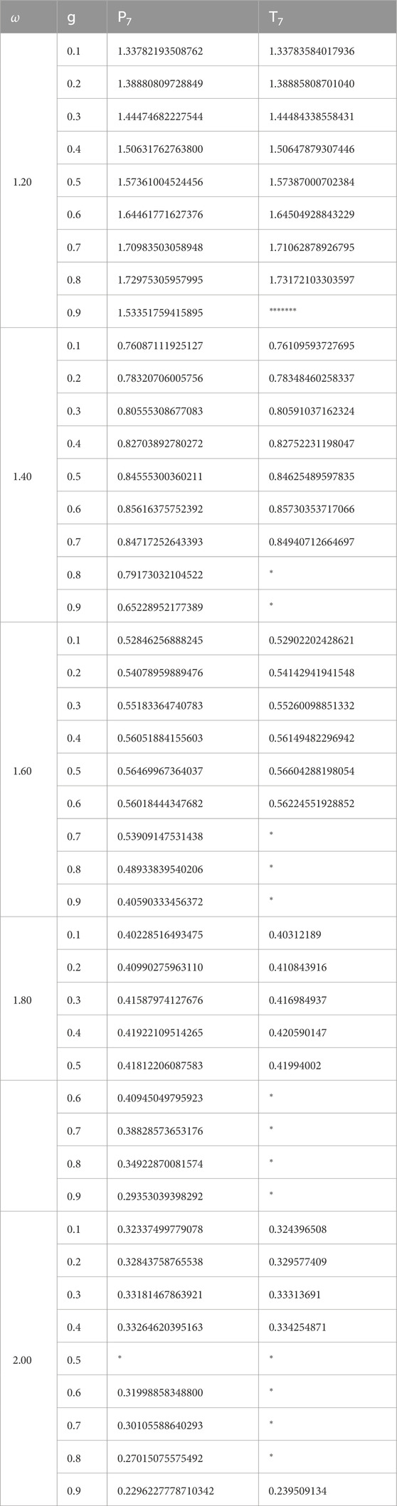
Table 2. Comparison of the radiative thickness $\tau$ for HG scattering with P_N and T_N methods.

A comparison of the results for the AG phase function is presented in Table 3. The consistency observed between the PN and TN methods is comparable to that of the HG phase function, indicating that the AG phase function performs as robustly as the HG phase function within the framework of the RTE. This finding is of particular significance, given the historical use of the AG phase function in neutron transport studies. Its extension to radiative transfer systems thus represents a novel contribution to the field.

Table 3

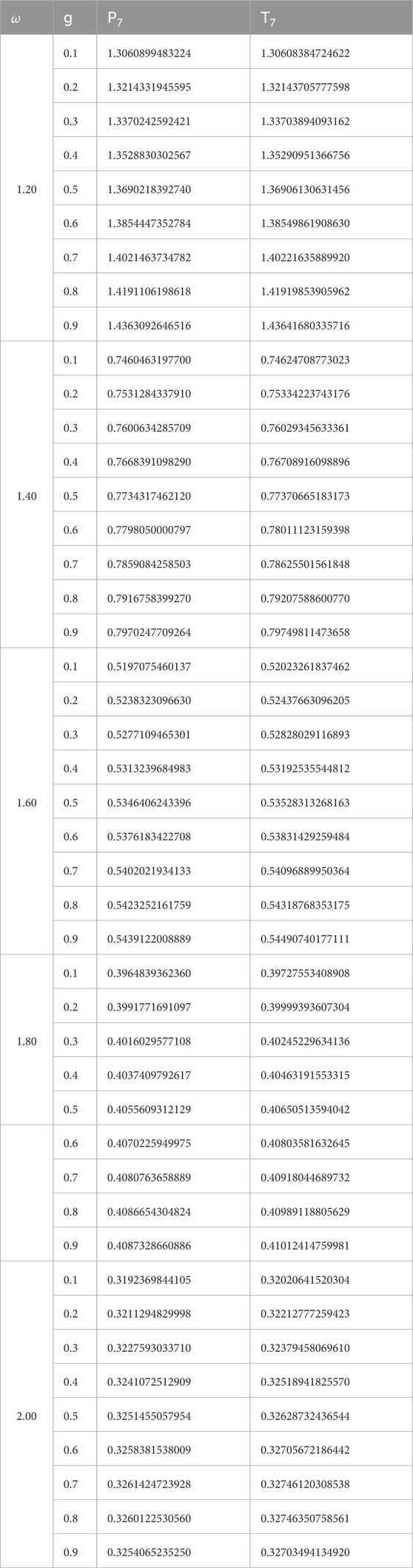
Table 3. Comparison of the radiative thickness $\tau$ for AG scattering with PN and TN methods.

In order to facilitate a more profound comprehension of the interrelationship between the values in the table, they have been represented graphically in Figure 2. As demonstrated by the graphs, the findings obtained from the methodologies employed for both scattering categories exhibit a consistent relationship with each other.

Figure 2

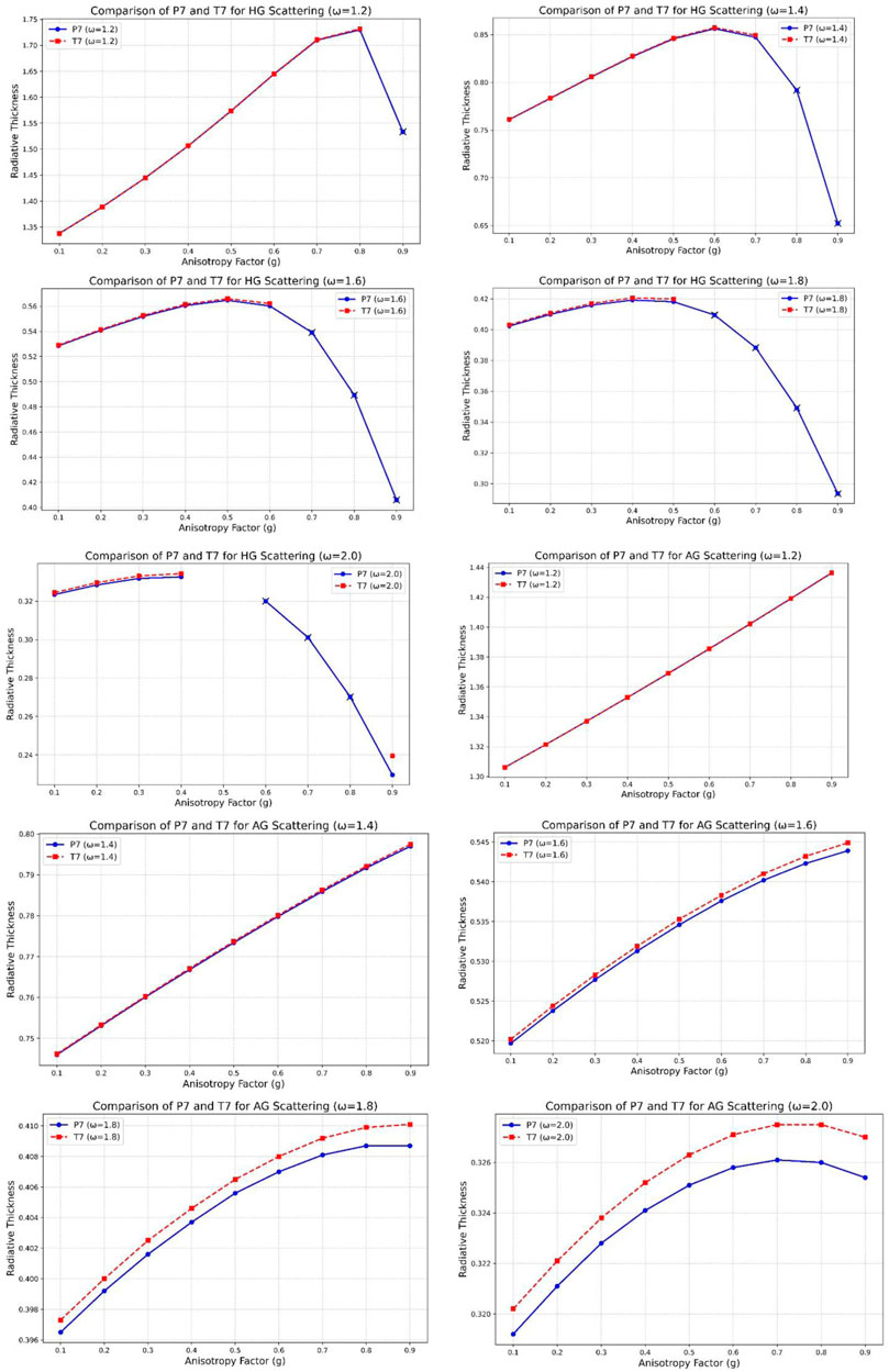
Figure 2. Comparison of the radiative thickness $\tau$ versus the g parameter for HG and AG scattering with the P_N and T_N methods.

For the HG phase function, the radiative thickness values obtained with the TN method are consistently higher than those obtained via the PN method across all ω values. The difference becomes more pronounced as both the anisotropy parameter g and ω increase. Notably, for ω = 1.2 and ω = 1.4, the TN results begin to deviate significantly at higher g, which may indicate increased angular sensitivity and stronger directional scattering captured by the TN method. Additionally, several missing values in the TN results, especially at high g, may be attributed to numerical instability or limitations in capturing sharp scattering features. Under the AG phase function, both PN and TN methods produce very similar and smooth results. The radiative thickness values increase monotonically with g, and the difference between PN and TN is minimal throughout the entire domain. This consistency suggests that the AG phase function leads to a numerically stable formulation and performs reliably across different discretization schemes. The close agreement of PN and TN outputs under AG further supports the suitability of the AG model for problems requiring robust and consistent predictions.

Overall, while the HG phase function exhibits greater sensitivity to the choice of angular discretization method, especially in anisotropic regimes, the AG phase function delivers smoother and more compatible solutions across both PN and TN schemes.

As demonstrated in Figure 3, the optical thickness values obtained from the numerical solutions are presented as a function of angular flux and thickness. Note that the values where the function passes through zero on the graphs are identical to the thickness values obtained for specific values of w and g.

Figure 3

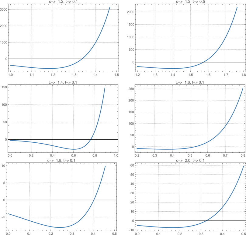
Figure 3. The graphs of the angular flux $I\left(x,\mu \right)$ function to the critical thickness $\tau .$

As demonstrated in Tables 2, 3, the outcomes of the two methods are closely aligned, indicating a high degree of concordance between them. This finding suggests that the solution to the RTE employing Chebyshev polynomials yields results that are consistent with those obtained through the Legendre polynomial method. The second result obtained from the study is the applicability of the AG phase function to the RTE solution. As demonstrated in both the tables and graphs, the results obtained from these two methods are consistent with each other. It is also evident from the analysis that the radiative thickness solution constitutes a distinct framework for the RTE solution. The solutions obtained from both methods and the two different phase functions demonstrate consistency with each other. Consequently, researchers with a keen interest in this area can easily compare the solutions presented in this study and their own methods.

4 Conclusion

This study presents a novel solution to the radiative transfer equation (RTE), namely, the radiative thickness solution, which offers a significant contribution to the existing body of knowledge. While previous studies have extensively discussed reflectivity, transmittance, and albedo, this work provides a novel focus on radiative thickness, which has been largely overlooked in the context of slab or multilayer slab geometries. It is anticipated that our findings will serve as a benchmark for researchers engaged in similar systems and methodologies, facilitating comparisons. The reliability and consistency of the methods employed in this study reinforce the applicability of our results to a range of fields, including atmospheric radiative transfer and radiative transfer in biological tissues.

The solutions presented in this study are based on the Henyey–Greenstein (HG) phase function, which is the most widely applied and accepted scattering model in RTE analyses. The use of the HG phase function ensures broad applicability, as it is highly relevant for both theoretical studies and practical implementations. Two distinct numerical methods were employed to solve the RTE, and the excellent agreement between the results validates the robustness of these methods. Furthermore, this work incorporates solutions for the AG phase function, which has gained prominence in neutron transfer studies due to its favorable performance. The compatibility of results obtained using the AG phase function provides additional support for the validity and versatility of our approach.

It is believed that our study contributes a new scattering phase function for RTE studies. Anlı-Güngör scattering is used for neutron transport solutions. The use of Anlı-Güngör scattering in the RTE is new in the area. The study showed the applicability of this phase function for the radiative transfer equation solutions. The accuracy of the result is controlled by comparing the two different methods.

Furthermore, the study underscores the significance of pivotal parameters in the RTE, including the anisotropy parameter g and the single scattering albedo w. The anisotropy parameter, which is pivotal for modeling radiative transfer in atmospheric and biological tissues, was evaluated across the entire range with a step size of 0.1. This granular approach provides a comprehensive understanding of the behavior of the radiative thickness in the presence of varying anisotropic conditions. Similarly, the single scattering albedo, an essential parameter in radiative transfer studies, was calculated in 0.2 intervals for values up to two, encompassing the range most frequently utilized in the literature. The comprehensive tabulation of these results serves as a valuable reference for future research endeavors.

In conclusion, this work not only addresses a significant gap in the study of RTE but also establishes a robust framework for future research. It is anticipated that the comprehensive benchmark values presented in this study will serve as a source of inspiration for further investigations and innovations in radiative transfer modeling.

Data availability statement

All data supporting the conclusions of this article are included within the article itself. Further inquiries can be directed to the corresponding author.

Author contributions

HK: Conceptualization, Methodology, Formal analysis, Visualization, Writing – original draft, and Writing – review and editing.

Funding

The author(s) declare that no financial support was received for the research and/or publication of this article.

Conflict of interest

The author declares that the research was conducted in the absence of any commercial or financial relationships that could be construed as a potential conflict of interest.

Generative AI statement

The author(s) declare that no Generative AI was used in the creation of this manuscript.

Publisher’s note

All claims expressed in this article are solely those of the authors and do not necessarily represent those of their affiliated organizations, or those of the publisher, the editors and the reviewers. Any product that may be evaluated in this article, or claim that may be made by its manufacturer, is not guaranteed or endorsed by the publisher.

References

1. Ishimaru A. Wave propagation and scattering in random media, 1. Academic Press (1978) 309 Chap. 2. p. 25.

Google Scholar

2. Klose AD, Hielscher AH. Quasi-analytical solutions for time-resolved photon migration in 3D turbid media. Int J Numer Methods Heat & Fluid Flow (2008) 18(5):443–57. doi:10.1108/09615530810872291

CrossRef Full Text | Google Scholar

3. Kumar S, Srivastava A. Radiative heat transfer in a plane-parallel medium using the spectral Chebyshev method. Int J Heat Mass Transfer (2015) 90:466–75. doi:10.1016/j.ijheatmasstransfer.2015.06.025

CrossRef Full Text | Google Scholar

4. Milne EA. Radiative equilibrium in the outer layers of a star: the temperature distribution and the law of darkening. Monthly Notices R Astronomical Soc (1921) 81(5):361–75. doi:10.1093/mnras/81.5.361

CrossRef Full Text | Google Scholar

5. Chandrasekhar S. The radiative equilibrium of a stellar atmosphere. Monthly Notices R Astronomical Soc (1934) 94(5):444–59. doi:10.1093/mnras/94.5.444

CrossRef Full Text | Google Scholar

6. Kosirev NA. Radiative equilibrium of the extended photosphere. Monthly Notices R Astronomical Soc (1934) 94(5):430–43. doi:10.1093/mnras/94.5.430

CrossRef Full Text | Google Scholar

7. Schuster A. Radiation through a foggy atmosphere. The Astrophysical J (1905) 21(1):1–22. doi:10.1086/141186

CrossRef Full Text | Google Scholar

8. Liemert A, Kienle A. Analytical solution of the radiative transfer equation for infinite-space fluence. Phys Rev A (2011) 83(1):015804. doi:10.1103/PhysRevA.83.015804

CrossRef Full Text | Google Scholar

9. Ma D, Li D, Ding H, Guo K, Liu B, Guo Z. Polarization sensing underwater target penetrating complex droplet-bubble layer. IEEE Sensors J (2024) 24:41836–47. doi:10.1109/JSEN.2024.3483937

CrossRef Full Text | Google Scholar

10. Tavanti E, Caviglia DD, Randazzo A. Improved Chebyshev spectral method modeling for vector radiative transfer in atmospheric propagation. IEEE Trans Antennas Propagation (2024) 72(5):4465–76. doi:10.1109/TAP.2024.3378831

CrossRef Full Text | Google Scholar

11. Zhang D, Rahnema F. Continuous-energy time-dependent coarse mesh transport (COMET) method for kinetics calculations. Nucl Sci Eng (2024) 198(3):565–77. doi:10.1080/00295639.2023.2196935

CrossRef Full Text | Google Scholar

12. Bardin R, Bertrand F, Palii O, Schlottbom M. A phase-space discontinuous Galerkin scheme for the radiative transfer equation in slab geometry. Comput Methods Appl Mathematics (2024) 24(3):557–76. doi:10.1515/cmam-2023-0090

CrossRef Full Text | Google Scholar

13. Allakhverdian V, Naumov DV. Infinite series solution of the time-dependent radiative transfer equation in anisotropically scattering media. J Quantitative Spectrosc Radiative Transfer (2024) 326:109126. doi:10.1016/j.jqsrt.2024.109126

CrossRef Full Text | Google Scholar

14. Chandrasekhar S. Radiative transfer. Oxford University Press (1950).

Google Scholar

15. Modest MF. Radiative heat transfer. 2nd ed. Academic Press (2003).

Google Scholar

16. De Florio M, Schiassi E, Furfaro R, Ganapol BD, Mostacci D. Solutions of Chandrasekhar’s basic problem in radiative transfer via theory of functional connections. J Quantitative Spectrosc Radiative Transfer (2020) 259:107384. doi:10.1016/j.jqsrt.2020.107384

CrossRef Full Text | Google Scholar

17. Balsara D. Fast and accurate discrete ordinates methods for multidimensional radiative transfer. Part I: basic methods. J Quantitative Spectrosc Radiative Transfer (2001) 69(6):671–707. doi:10.1016/S0022-4073(00)00114-X

CrossRef Full Text | Google Scholar

18. Lathrop KD. Use of discrete ordinates and spherical harmonics in the solution of the neutron transport equation. Nucl Eng Des (1965) 15(3):335–42. doi:10.1016/0029-5493(65)90013-3

CrossRef Full Text | Google Scholar

19. Kumar S, Tien CL, Majumdar A. Radiative heat transfer in semitransparent media with nonuniform refractive index. J Heat Transfer (1990) 112(2):199–205. doi:10.1115/1.2910413

CrossRef Full Text | Google Scholar

20. Williams MMR, Hall SK, Eaton MD. Solution of the two-dimensional diffusion and transport equations in hexagonal geometry. Annals Nucl Energy (2014) 63:146–56. doi:10.1016/j.anucene.2013.08.012

CrossRef Full Text | Google Scholar

21. Stamnes K. Numerical methods for forward models. In: Lecture presented at the course on inverse methods in atmospheric science. Trieste, Italy: International Centre for Theoretical Physics ICTP (2001). Retrieved from: https://indico.ictp.it/event/a01105/material/4/3.pdf.

Google Scholar

22. Haghighat A. Monte Carlo methods for particle transport. 2nd ed. Boca Raton, FL: CRC Press (2020). doi:10.1201/9780429198397

CrossRef Full Text | Google Scholar

23. Heningburg V. Numerical methods for radiative transport equations (Doctoral dissertation). Knoxville, TN: University of Tennessee (2019). Available online at: https://trace.tennessee.edu/utk_graddiss/.

Google Scholar

24. Kim AD, Moscoso M. Chebyshev spectral methods for radiative transfer. Arbor, MI: SIAM J Scientific Computing (2002) 23(6):2074–94. doi:10.1137/S1064827500382312:c

CrossRef Full Text | Google Scholar

25. McClarren RG. Spherical harmonics methods for thermal radiation transport. Doctoral dissertation. Ann Arbor, MI: University of Michigan (2006).

Google Scholar

26. Gantri M. Solution of radiative transfer equation with a continuous and stochastic varying refractive index by Legendre transform method. Comput Mathematical Methods Medicine (2014) 2014:1–7. doi:10.1155/2014/814929

PubMed Abstract | CrossRef Full Text | Google Scholar

27. Tapimo R, Kamdem HTT, Yemele D. Discrete spherical harmonics method for radiative transfer in scalar planar inhomogeneous atmosphere. J Opt Soc America A (2018) 35(7):1081–90. doi:10.1364/JOSAA.35.001081

PubMed Abstract | CrossRef Full Text | Google Scholar

28. Siewert CE. A discrete-ordinates solution for radiative transfer models that include polarization effects. J Quantitative Spectrosc Radiative Transfer (2001) 70(2):123–32. doi:10.1016/S0022-4073(01)00056-4

CrossRef Full Text | Google Scholar

29. Binzoni T, Leung TS, Gandjbakhche AH, Rüfenacht D, Delpy DT. The use of the Henyey–Greenstein phase function in Monte Carlo simulations in biomedical optics. Phys Medicine & Biol (2006) 51(17):N313–22. doi:10.1088/0031-9155/51/17/N04

PubMed Abstract | CrossRef Full Text | Google Scholar

30. Anli F, Yasa F, Güngör S. General eigenvalue spectrum in a one-dimensional slab geometry transport equation. Nucl Sci Eng (2005) 150(1):72–7. doi:10.13182/NSE05-A2502

CrossRef Full Text | Google Scholar

31. Pomraning GC. Transport theory. University of California Press (1973).

Google Scholar

32. Henyey LG, Greenstein JL. Diffuse radiation in the galaxy. Astrophysical J (1941) 93:70–83. doi:10.1086/144246

CrossRef Full Text | Google Scholar

33. Tuchin VV. Light interaction with biological tissues: overview. Proc SPIE Vol. 1884: Static Dynamic Light Scattering Medicine Biol (1993) 1884:234–72. doi:10.1117/12.148348

CrossRef Full Text | Google Scholar

34. Elghazaly A. Anisotropic radiative transfer in a finite inhomogeneous slab using the Legendre polynomial method. J Quantitative Spectrosc Radiative Transfer (2009) 110(12):2021–30. doi:10.1016/j.jqsrt.2009.05.007

CrossRef Full Text | Google Scholar

35. El-Wakil SAMTA, Ablilwafa EM. Radiative transfer in a finite plane-parallel medium with anisotropic scattering. Radiat Phys Chem (2010) 82(1):34–40. doi:10.1016/j.radphyschem.2010.09.003

CrossRef Full Text | Google Scholar

36. Liemert A, Kienle A. Analytical Green’s function of the radiative transfer radiance for the infinite medium. Phys Rev E (2011) 83(3):036605. doi:10.1103/PhysRevE.83.036605

PubMed Abstract | CrossRef Full Text | Google Scholar

37. Liemert A, Reitzle D, Kienle A. Analytical solutions of the radiative transport equation for turbid and fluorescent layered media. Scientific Rep (2017) 7:3819. doi:10.1038/s41598-017-02979-4

PubMed Abstract | CrossRef Full Text | Google Scholar

38. Ge W, Marquez R, Modest MF, Roy SP. Implementation of high-order spherical harmonics methods for radiative heat transfer on OpenFOAM. J Heat Transfer (2015) 137(5):052701. doi:10.1115/1.4029546

CrossRef Full Text | Google Scholar

39. Machida M, Panasyuk GY, Schotland JC, Markel VA. The Green's function for the radiative transport equation in the slab geometry. J Phys A: Mathematical Theor (2010) 43(6):065402. doi:10.1088/1751-8113/43/6/065402

CrossRef Full Text | Google Scholar

40. Liemert A, Kienle A. Analytical approach for solving the radiative transfer equation in two-dimensional layered media. J Quantitative Spectrosc Radiative Transfer (2012) 113(7):559–64. doi:10.1016/j.jqsrt.2012.01.002

CrossRef Full Text | Google Scholar

41. Liemert A, Kienle A. Exact and efficient solution of the radiative transport equation for the semi-infinite medium. Scientific Rep (2013) 3:2018. doi:10.1038/srep02018

PubMed Abstract | CrossRef Full Text | Google Scholar