Geometric structure of parameter space in immiscible two-phase flow in porous media

In a recent paper, a continuum theory of immiscible and incompressible two-phase flow in porous media based on generalized thermodynamic principles was formulated (Transport in Porous Media, 125, 565 (2018)). In this theory, two immiscible and incompressible fluids flowing in a porous medium are treated as a single effective fluid, substituting the two interacting subsystems for a single system with an effective viscosity and pressure gradient. In assuming Euler homogeneity of the total volumetric flow rate and comparing the resulting first-order partial differential equation to the total volumetric flow rate in the porous medium, one can introduce a novel velocity that relates the two pairs of velocities. This velocity, the co-moving velocity, describes the mutual co-carrying of fluids due to immiscibility effects and interactions between the fluid clusters and the porous medium itself. The theory is based upon general principles of classical thermodynamics and allows for many relations and analogies to draw upon in analyzing two-phase flow systems in this framework. The goal of this work is to provide additional connections between geometric concepts and the variables appearing in the thermodynamics-like theory of two-phase flow. In this endeavor, we will encounter two interpretations of the velocities of the fluids: as tangent vectors (derivations) acting on functions or as coordinates on an affine line. The two views are closely related, with the former viewpoint being more useful in relation to the underlying geometrical structure of equilibrium thermodynamics and the latter being more useful in concrete computations and finding examples of constitutive relations. We apply these relatively straightforward geometric contexts to interpret the relations between velocities and, from this, obtain a general form for the co-moving velocity.

1 Introduction

The formulation of an effective continuum-level theory of immiscible and incompressible two-phase flow in porous media based on rigorous physical principles is a problem of great importance spanning several disciplines within physics and mathematics [1–4]. The behavior of such flows underpins a range of complex phenomena seen in nature, industrial applications, and general theoretical models where one can map a problem onto a description where two interacting populations, here fluids, are exploring a constrained and complex network.

Flow in porous media has a long history. The earliest study of porous media we know of is that of Reinhard Woltmann, who introduced the concept of volume fractions in connection with the movement of water sediments in 1794 [5]. Sixty years later, Henri Darcy found a linear relation between single-phase flow rate and pressure drop in sand packings [6]. His result may be expressed as a local constitutive equation relating flow velocity and pressure gradient,

$\vec{v}=-\frac{K}{\mu \varphi }\nabla P,(1)$

where $\vec{v}$ is the seepage (or pore) velocity of the fluid, $P$ the pressure, $K$ the permeability, $\varphi$ the porosity, and $\mu$ the fluid viscosity. Two-phase flow in the form of water and air in soils entered the literature with the works of Buckingham in 1907 [7], where he introduced capillarity as a central concept. He also made the first attempts at formulating a generalization of the Darcy law for unsaturated flow. Richards wrote equations for the unsaturated movement of water in soil in 1931 [8], which are still in use in this context today. In 1936, Wyckoff and Botset [9] made the first steps toward relative permeability theory, followed by Muscat and Meres [10], who introduced the concept of relative permeability, generalizing the “capillary conductance” concept that Buckingham introduced [7]. Leverett introduced the capillary pressure curve [11] into the framework of Muscat and Meres in 1941, completing the theory as it is used in practical calculations today.

We summarize the relative permeability theory in the following. We have two immiscible and incompressible fluids, one more wetting with respect to the porous matrix than the other. We refer to them as the wetting (w) and non-wetting (n) fluids. From the perspective of one of the fluids, the pore space it sees is the total pore space of the porous medium minus the pore space occupied by the other fluid, and vice versa. The relative reduction of pore space for each fluid implies a reduction in effective permeability for each fluid, leading to the two constitutive equations, which are generalizations of the Darcy Equation 1; [4].

${\vec{v}}_w=-\frac{K{k}_{rw}}{{\mu }_w\varphi S_w}\nabla P_w,(2)$

${\vec{v}}_n=-\frac{K{k}_{rn}}{{\mu }_n\varphi S_n}\nabla P_n,(3)$

where ${\vec{v}}_w$ and ${\vec{v}}_n$ are the seepage velocities of the wetting and non-wetting fluids, respectively, ${\mu }_w$ and ${\mu }_n$ are the viscosities of each fluid, respectively, $P_w$ and $P_n$ are the pressure in each fluid, respectively,$S_w$ and $S_n$ are the wetting and non-wetting saturations, and $k_{rw}$ and $k_{rn}$ are the relative permeabilities of the two fluids, respectively.

The saturations $S_w$ and $S_n$ are defined as the fraction of pore space occupied by each fluid so that

$S_w+S_n=1.(4)$

If the relative permeabilities depend on the saturation $S_w$ and the pressures $P_w$ and $P_n$, that is, $k_{rw}(S_w,P_w,P_n)$ and $k_{rn}(S_w,P_w,P_n)$, the constitutive Equations 2, 3 will be generic in the sense that any constitutive pair of constitutive equations may be written in this form. They do, however, gain physical content if the assumption is made that they depend only on the saturations, that is, $k_{rw}(S_w)$ and $k_{rn}(S_w)$. This is the assumption made in all practical calculations.

The difference in pressure between the two fluids is defined as the capillary pressure curve $P_c$,

$P_n-P_w=P_c\left(S_w\right).(5)$

It is also assumed in practical calculations that the capillary pressure curve depends on the saturation $S_w$ only. The capillary pressure curve is a particularly difficult quantity, both conceptually and in terms of measurement [12].

We define the average pore velocity $\vec{v}$ as

$\vec{v}=S_w{\vec{v}}_w+S_n{\vec{v}}_n,(6)$

That is, we are using a volume average because we are assuming the fluids to be incompressible, allowing us to avoid the fluid densities entering the equations,

$\nabla \cdot \left[\varphi {\vec{v}}_p\right]=0.(7)$

Volume conservation gives

$\varphi \frac{\partial S_w}{\partial t}+\nabla \cdot \left[\varphi S_w{\vec{v}}_w\right]=0,(8)$

$\varphi \frac{\partial S_n}{\partial t}+\nabla \cdot \left[\varphi S_n{\vec{v}}_n\right]=0,(9)$

where $t$ is time. The set of Equations 2–9 is closed as long as $k_{rw}(S_w)$, $k_{rn}(S_w)$, and $P_c(S_w)$ are provided.

Going beyond these phenomenological theories has turned out to be difficult. The dominating approach is that of homogenization, either based on pore-level momentum transfer [13–17] or pore-level energy transfer [18–21]. The pore-scale equations, either based on hydrodynamics (momentum transfer) or thermodynamics (energy transfer), must then be averaged; see Whitaker [22, 23]. This averaging is based on equating the average of the gradient of a variable associated with pore space to the gradient of the average variable plus an integral over the surface area of the pores. Because the surface area of porous media typically scales as the volume, this integral does not vanish as one moves up in scale. The variable appearing in the surface integral is then split into an average and a fluctuating part, resulting in the average and gradients of the average being expressed in terms of the fluctuations of the original variable. A closure assumption is then necessary that relates the fluctuations to the average independently.

Another important homogenization approach based on thermodynamics is thermodynamically constrained averaging theory (TCAT) [24–27].

McClure et al. [28, 29] emphasize that homogenization should also include averaging over time and point out that different processes are associated with different time scales: the larger the scales, the longer the averaging time will be.

In another approach, McClure et al. [30] derive the relative permeability equations from an energy budget based on thermodynamic considerations and homogenization. The relative permeability equations do appear as a first term in a series expansion. However, it is not shown in [30] that the higher-order terms are negligible.

The topology of a porous medium seen as a geometrical object may be described using the four Minkowski functionals: volume, surface area, mean curvature, and the Euler characteristics. The Hadwiger theorem states that the Minkowski functionals form a complete basis set for all extensive functions that are invariant with respect to the orientation of the object [31]. The use of this theorem to characterize the free energy of fluids in a porous medium combined with homogenization constitutes another approach to the scale-up problem [32–35].

An approach circumventing the complexities associated with homogenization is based on classical non-equilibrium thermodynamics [36–40]. By using the extensiveness of the internal energy of the fluids, the Euler theorem for homogeneous functions allows for defining thermodynamic variables such as pressure and chemical potentials on the Darcy scale. Gradients in the intensive variables are introduced, and the machinery of classical non-equilibrium thermodynamics [36, 37] is then used. The underlying homogenization is somewhat hidden in this approach, but it underlies the way a representative elementary volume (REV) is defined and used.

Homogenization leads to complex equations with many variables. The root of this difficulty is that homogenization can only produce averages over the original variables. There is no inherent mechanism built into it that can produce emergent variables that capture emergent properties [41].

A very different approach to the scale-up problem, that is, deriving a Darcy (or continuum) scale description of immiscible two-phase flow in porous media from the physics at the pore level, is based on statistical mechanics [42, 43]. Statistical mechanics was originally developed for the bridge between a molecular description of thermal systems and thermodynamics, which is a continuum-scale theory. Continuum-scale variables such as temperature and pressure emerge naturally in this framework. Jaynes generalized statistical mechanics from being specifically constructed for molecular systems to any system fulfilling a set of conditions [44]. In the context of immiscible and incompressible two-phase flow in porous media, the Jaynes generalized statistical mechanics could be implemented when the flow was assumed to be in a steady state [45–48]. By this, we mean that the two immiscible fluids are mixed in such a way that no continuum-scale saturation gradients exist. It does not mean that the interfaces between the fluids remain fixed. Rather, Avraam and Payatakes [45] classified steady-state flow into different flow regimes: connected pathway flow, ganglion dynamics flow, and drop traffic flow. Only in the first one, characterized by slow flow, are the interfaces stuck. In the ganglion dynamics regime, the fluids form clusters larger than the pores, which break up and merge. The fast-flow drop traffic regime is characterized by one of the fluids having broken up into small droplets that move in traffic-like patterns.

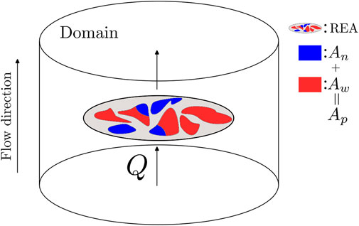
A necessary condition for implementing the Jaynes approach is to demonstrate that entropy is not generated by the system. Under any kind of flow conditions, steady state or not, molecular entropy is generated through viscous dissipation and movement of contact lines at the pore level. However, consider a cylindrical porous medium sample. We consider an area orthogonal to the average flow direction along the cylinder axis. The pores are filled with wetting fluid or non-wetting fluid. The distribution of the pores, the fluids within the pores, and the accompanying velocity field may be characterized by a configurational entropy in the sense of Shannon [49]. This configurational entropy is not produced when the flow is under steady-state conditions. Using the area covered by the pore $A_p$, the area cutting through the wetting fluid $A_w$, and the area cutting through the non-wetting fluid $A_n$, so that $A_w+A_n=A_p$, the wetting and non-wetting volumetric flow rates through the area, $Q_w$ and $Q_n$, so that $Q_w+Q_n=Q_p$, which is the total volumetric flow rate as variables extensive in the area $\tilde{A}$, we may build a statistical mechanics upon them using the maximum (configurational) entropy assumption. In the process, emergent intensive variables appear. More than that, a complete thermodynamics-like description appears at the continuum level. By this, we mean relations between the intensive and extensive variables that closely resemble those of thermodynamics. We will refer to this thermodynamics-like framework as a pseudo-thermodynamics.

In 2018, Hansen et al. [50] used extensivity to derive a number of pseudo-thermodynamics relations between the seepage velocities of the fluids, $v_w$ and $v_n$, and the saturation $S_w$. This work should be seen as a precursor to [42, 43]. It is this work that the present article will focus on. Central to it was to provide a two-way mapping between the two seepage velocities $v_w$ and $v_n$ and the average seepage velocity $v$. Assuming the flow is along the cylinder axis and Equation 6 may be written

$v=S_w{v}_w+S_n{v}_n.(10)$

This provides the mapping $(v_w,v_n)\to v$. The generalized Darcy Equations 2, 3 provide constitutive equations for $v_w$ and $v_n$, and Equation 6, or Equation 10, then provides a constitutive equation for the average velocity $v$. It is, however, not possible uniquely to construct the inverse mapping $v\to (v_w,v_n)$.

A central accomplishment in [50] was to deduce the existence of a new velocity, the co-moving velocity $v_m$, to pair with the average velocity $v$, thus making the inverse mapping $(v,v_m)\to (v_w,v_n)$ possible.

$v_w=v+S_n\left[\frac{\partial v}{\partial S_w}-v_m\right],(11)$

$v_n=v-S_w\left[\frac{\partial v}{\partial S_w}-v_m\right].(12)$

The mapping $(v_w,v_n)\to v$, on the other hand, is complemented by the mapping $(v_w,v_n)\to v_m$,

$v_m=S_w\frac{\partial v_w}{\partial S_w}+S_n\frac{\partial v_n}{\partial S_w}.(13)$

Equations 10–13 form the two-way mapping $(v_w,v_n)\leftrightarrow (v,v_m)$.

Why would one want to construct the inverse mapping, $(v,v_m)\to (v_w,v_n)$? It was observed experimentally in 2009 [46, 51] that the average seepage velocity $v$ follows a power law in the pressure gradient with an exponent considerably larger than one (as would be the case for Darcy flow) over a wide range of capillary numbers. This observation has been followed up in multiple articles; see, for example, [52–60]. Experimentally, one finds this power-law behavior around a capillary number of the order of $10^{-5}$ and up. The power law appears when an increase in pressure gradient results in the mobilization of interfaces that would otherwise be held in place by the capillary forces. If we assume that the increase in mobilized interfaces is proportional to the increase in pressure gradient and the increase in effective permeability is proportional to the increase in mobilized interfaces, we end up with an exponent equal to two. The flow rate-pressure gradient reverts to being linear again when all interfaces that may move are moving [55]. Having the mapping from $(v,v_m)$ to $(v_w,v_n)$, Equations 11, 12, make it possible to reconstruct the seepage velocity constitutive equations for each fluid from the constitutive equation between $v$ and the pressure gradient.

An important remark here is that both ordinary thermodynamics and the pseudo-thermodynamics formalism for porous media flow provide a general set of relations between the variables involved, for example, Equations 10–13. These relations then must be supplemented by constitutive equations in order to describe a particular flow problem. This is what relative permeability theory provides, and this has also been the aim of homogenization efforts. The aim of the statistical mechanics approach to porous media flow and its ensuing pseudo-thermodynamics so far has not been to provide the constitutive equations but rather to build a framework in which they may be placed. Thus, the generalized Darcy Equations 2, 3 could be a possible choice.

To verify whether a thermodynamic framework can support the inclusion of these constitutive relations, one must consider the mathematical backbone of thermodynamics to check whether such as this can be justified and whether it is possible to reproduce or obtain new results using this framework. This backbone is, in fact, based on geometry, framed in terms of abstract manifolds, structures on these spaces, and potential symmetries of the relations of the theory. Hence, these are natural objects to consider.

The perhaps most important observation of the pseudo-thermodynamic two-phase flow problem is that homogeneity plays a central role, which amounts to imposing a scaling behavior on the variables. Hence, if one is concerned with the velocities of the fluids in the porous medium, scaling can be viewed as a symmetry of the system. Moreover, affine forms of the involved functions often appear in the two-phase flow problem, for instance, if the total volumetric flow rate has an irreducible flow rate that does not scale homogeneously [50, 61]. Scaling symmetry, in particular, is a strong motivator for seeking a geometric description of the problem. Ideally, such a description should be framed in a form appropriate for generalization to more thermodynamic variables [62] while possibly admitting a formulation that makes it possible to obtain novel constitutive relations for the co-moving velocity with respect to the allowed transformations of the variables of the problem. Lastly, unlike earlier work on the geometric formulation of the problem [63], we here seek a structure where there is a mathematical distinction between the extensive and intensive variables.

To investigate these possibilities in this article, we will reframe the theory of [50] using the basic concepts from two related geometric viewpoints. The first one is the basic differential geometry and (tangent) bundle structure of the configuration space of extensive variables, where the velocities correspond to tangent vector fields. The second one is a classical geometric view of the velocities as points in an affine space. Due to the simplicity of the configuration spaces considered in this article, the latter can be viewed as a “global” formulation of the former “local” description. In essence, the local description in terms of tangent vectors can be extended to the global description by treating the integral curves of the tangent vectors, which define lines in terms of a set of coordinates that are “dual” or “conjugate” to the extensive variables. This description will not be laid out in detail in this article (see Section 3.3 for a basic introduction) and is mostly left for future work. We will only need basic concepts from both the classical and differential viewpoints; the difficulty here is not mathematical but rather lies in the physical interpretation of the results¹.

The unifying principle in the two approaches is the assumption of degree-1 homogeneity in the total volumetric flow rate. Moreover, it is assumed that one can switch between a global and a differential formulation without complications, meaning, in essence, that the underlying space of extensive variables is trivial. In this article, this means that this space is isomorphic to ${\mathbb{R}}^n$, as considered in earlier works [63]. Hence, the thermodynamic velocities obtained from the Euler homogeneous function theorem and from the exact differential corresponding to the volumetric flow rate are equal. This is the essential content of assuming that $Q$ is extensive in the pore areas.

In the thermodynamic description, the thermodynamic velocities are equations of state (EOSs). The seepage velocities are related to driving forces in the system through constitutive relations. By viewing these driving forces as externally fixed parameters and letting the velocities be functions of the saturation only, the problem is equivalent to a kinematics problem with the saturation as the parameter determining the dynamics². In other words, saturation plays the role of a “time” parameter, and homogeneity is necessary to introduce this quantity. Hence, a geometric formulation of the flow problem in terms of a single variable occurs naturally if extensivity is taken as a basic tenet of the theory. This is especially convenient if saturation is the control variable, and it will be shown that this assumption simplifies both the local and global formulation of the problem as much as possible.

The local (differential) description, in particular, can be further distinguished by the view of the total volumetric flow rate either as defining an equation-of-state surface $Q=Q\left(A_w,A_n\right)$ in a space of extensive variables $\left(Q,A_w,A_n\right)$ or as a function on the space of extensive variables $\left(A_w,A_n\right)$. The difference between the two viewpoints is that they are extrinsic or intrinsic views of the configuration space and give the theory slightly different flavors. However, picking one or the other does not radically alter the interpretations of the involved quantities; the extrinsic view is obtained by extending the area-configuration space by an extra dimension. This dimension can be described via an additional extensive variable, and the image of $Q\left(A_w,A_n\right)$ is viewed as embedded in this extended configuration space as a $2D$ EOS surface. This surface can itself be the subject of study in a differential description [64]. This view will only be considered briefly in Section 5.1.

The “classical” geometric viewpoint in this work interprets the values of the functions corresponding to the velocities $v_w$, $v_n$, $v$ and $v_m$ as points in an affine space. The geometric relations are motivated by the particular form of the equations presented in Section 2.

We will see how both views, which use many of the same types of spaces but with different objects defined on them, can aid in our understanding of what the co-moving velocity, Equation 13, represents and how to potentially work with it. Moreover, we will see how this theory relates to a constitutive relation for the co-moving velocity

$v_m=b{v}^{\prime }+a{v}_0,(14)$

which has been found to be accurate to within the experimental and numerical precision available [61, 65, 66], and $v_0$ is a velocity scale.

The tangent–vector formulation can be seen in relation to previous works [67]. The difference here is that the tangent vectors are considered derivative operators, where the action of the tangent vector fields on functions defined on the space yields the velocities.

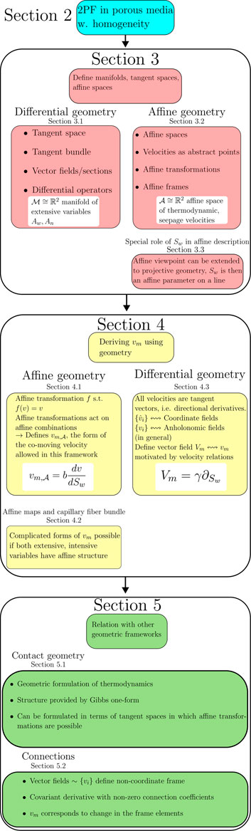
The structure of the article is as follows: in Section 2, we present the preliminaries of the pseudo-thermodynamic theory of two-phase flow [50], including the co-moving velocity itself and clarification on homogeneity and the separation of the total system into interacting subsystems. In Section 3, we introduce the machinery of manifolds, tangent and affine spaces, and bundles constructed from these spaces. These bundles are the natural habitats of the vector fields presented in this work, which will be represented in terms of partial derivatives with respect to the chosen coordinates. We will also present the preliminaries of using affine geometry in the classical geometric viewpoint, including affine spaces, affine transformations and how the velocities can be viewed and manipulated as abstract points. In Section 4, we show how the co-moving velocity appears in the two geometric viewpoints presented above and how it relates to the interpretation of the equations in Section 2. This is the main part of this work, with the goal of clearing up what the relations in Section 2 are seemingly stating in geometric terms and show how the co-moving velocity obtained in this way relates to already known relations.

Before summing up our results in Section 6, we will in Section 5 comment briefly on the usage areas of the results of Section 4. Moreover, we comment on two related topics to the concepts introduced in this work: how the results are related to contact geometry and the notion of a connection on a bundle. A high-level overview of Sections 2–5 is given in Figure 1.

Figure 1

Figure 1. A visual overview of the topics of each section of the article. Section II introduces the particular two-phase flow problem. Section III interprets the quantities and relations of Section II in terms of the two indicated geometric frameworks, with the goal of providing a better foothold for the generalization of the theory and connections with other systems subject to similar assumptions. In Section IV, the formalism introduced in Section III is used to obtain expressions for the co-moving velocity (white boxes), interpretable as a Euclidean vector and differential operator in the affine and differential descriptions, respectively. In Section V, the quantities of the theory are put into the context of contact geometry and connections, two topics that both represent ways of adding additional structure. This could provide a means for extending the formalism to describe phenomena like phase transitions in a geometric context.

2 Immiscible two-phase flow in porous media formulated as a thermodynamic problem

Consider a porous medium sample as shown in Figure 2. We assume the immiscible fluids enter through the bottom and leave through the top. The side walls are impenetrable. Within the porous medium, the fluids mix by forming clusters. The clusters merge and split, creating a steady state. We choose a plane orthogonal to the average flow direction far enough from the bottom so that it is in the region where the flow is in a steady state. In this plane, we choose a representative elementary area (REA), which is large enough for the macroscopic variables to have well-defined averages but not larger. The REA has an area $\tilde{A}$. We use the tilde to signify that the area $\tilde{A}$ is the area of a single plane. Associated with the REA, there is a time-averaged volumetric flow rate $Q$ of fluid passing through $\tilde{A}$ at each instant.

Figure 2

Figure 2. The porous medium sample with an REA indicated. The pore area $A_p$ can be divided into a wetting area $A_w$ and a non-wetting area $A_n$ so that their sum is $A_p$.

Figure 3

Figure 3. Scaling the area $A$ by a factor $\lambda$ scales the volumetric flow rate $Q$ in the same manner, demonstrating that $Q$ is a Euler homogeneous function of degree-1.

The average value of $\tilde{A}$ over the entire domain, defined as the integral of $\tilde{A}=\tilde{A}(z)$, where $z$ is the coordinate along the flow direction, is denoted by $A$. We will define all areas in this way, as their averaged values over the domain in the overall direction of $Q$ where the flow is in a steady state. We will in the following refer to the averaged area $A$ as the area of the REA. In the following, we will introduce several other kinds of areas. These will, in the same way, be averages over sets of REAs.

We define the porosity $\varphi$ of the porous medium as Equation 15:

$\varphi \equiv \frac{A_p}{A},(15)$

where $A_p$ is the area of $A$ that cuts through the pores. The solid matrix area $A_s$ is given by $A_s=A\left(1-\varphi \right)$. We assume the porous medium to be homogeneous. The pore area $A_p$ is an extensive variable; it scales with a factor $\lambda$ when we let $A\mapsto \lambda A$, where $\lambda$ is a real number. The porosity $\varphi$ does not change under this scaling; that is, it is an intensive variable.

The pore area of the REA, $A_p$, is split into an area $A_w$ of (more) wetting fluid and an area $A_n$ of (less) non-wetting fluid. The fluids are taken to be incompressible. We have that

$A_w+A_n=A_p.(16)$

We then define the wetting and non-wetting saturations as Equation 17 and 18.

$S_w=\frac{A_w}{A_p}=\frac{A_w}{\varphi A},(17)$

$S_n=\frac{A_n}{A_p}=\frac{A_n}{\varphi A},(18)$

obeying Equation 4.

Because we consider the mutual flow of two fluids, $Q$ can be decomposed as a sum of the volumetric flow rates of the individual fluids, denoted $Q_w$ and $Q_n$. We then have

$Q\left(A_w,A_n\right)=Q_w\left(A_w,A_n\right)+Q_n\left(A_w,A_n\right),(19)$

so $Q$ may be seen as a composite thermodynamic-like system consisting of two subsystems. We define the seepage velocities as

$v=\frac{Q}{A_p},(20)$

$v_w=\frac{Q_w}{A_w},(21)$

$v_n=\frac{Q_n}{A_n}.(22)$

These velocities of the individual fluids passing through the REA are the ones measured in experiments. We note that Equations 20–22 are not the Darcy (or superficial) velocities because one is not dividing by the total area $A$, but rather $A_p$, $A_w$, and $A_n$, which contain an additional factor of $\varphi$, $S_w\varphi$ and $S_n\varphi$, respectively. The weighted mean velocities in Equations 20–22 are often called interstitial velocities, advection velocities, or simply flow velocities and are equivalent to the (average) volumetric flux densities³ divided by the saturation. They are the mean velocities of the fluid elements passing through the REA⁴.

The total volumetric flow rate $Q$ is extensive in the variables $A_w$ and $A_n$, meaning that

$Q\left(\lambda A_w,\lambda A_n\right)=\lambda Q\left(A_w,A_n\right).(23)$

We are here assuming $A_w$ and $A_n$ to be the control variables. The pore area $A_p$ is then a dependent variable. This is, of course, not possible to arrange in the laboratory. However, theoretically, it is possible.

By defining $Q_w$, $Q_n$ in Equation 19 as functions of $A_w$, $A_n$ and not as $Q_w(A_w)$ and $Q_n\left(A_n\right)$, we imply that $Q$ is not a sum of simple, non-interacting subsystems [68]; the “subsystem” flow rates $Q_w$, $Q_n$ include interactions between the two phases of fluids. Taking a cue from thermodynamics, one could write $Q$ as the sum of two non-interacting volumetric flow rates $Q_{w,0}$, $Q_{n,0}$ and an interaction term $Q_{\text{int}}$

$Q\left(A_w,A_n\right)=Q_{w,0}\left(A_w\right)+Q_{n,0}\left(A_n\right)+Q_{\text{int}}\left(A_w,A_n\right).(24)$

Equation 24 requires physical input to determine the scaling properties of each term and is simply a formal separation of the system into two subsystems, one for each fluid [69]. Equation 23 still holds for the function $Q\left(A_w,A_n\right)$ by definition.

In general, a separation such as the one in Equation 24 is not possible to write down explicitly in all cases because the flow can be very complex. The only information we have is that the total volumetric flow rate $Q\left(A_w,A_n\right)$ scales as Equation 23. This identity does not exclude non-trivial scaling behavior or quasi-homogeneity [70] in each subsystem. Note that Equation 19 is formally not a separation into thermodynamic subsystems because the interaction between the systems is not explicitly accounted for, and both terms depend on both areas. Both Equations 19, 24 have the correct scaling behavior, but the difference lies in how the interaction is handled. One could, in theory, use Equation 24 for what follows; however, one only knows the relations in Equations 21, 22. We do not have such information about $Q_{w,0},Q_{n,0}$, which would allow us to determine $Q_{\text{int}}$. Hence, Equation 19 is used for what follows.

Using Equations 19–22, we find Equation 10. Equation 19 can then be rewritten as Equation 25:

$Q=A_w{v}_w+A_n{v}_n.(25)$

We now use the assumption that $Q$ is degree-1 Euler homogeneous in the areas [50], see Figure 3. Taking the derivative with respect to $\lambda$ on both sides of Equation 23 and setting $\lambda =1$, we get

$Q\left(A_w,A_n\right)=A_w{\left(\frac{\partial Q}{\partial A_w}\right)}_{A_n}+A_n{\left(\frac{\partial Q}{\partial A_n}\right)}_{A_w}.(26)$

By dividing Equation 26 by $A_p$, we get

$v=S_w{\left(\frac{\partial Q}{\partial A_w}\right)}_{A_n}+S_n{\left(\frac{\partial Q}{\partial A_n}\right)}_{A_w}.(27)$

The partial derivatives acting on $Q$ have units of velocity, so we define the thermodynamic velocities as Equations 28, 29:

${\widehat{v}}_w={\left(\frac{\partial Q}{\partial A_w}\right)}_{A_n},(28)$

and

${\widehat{v}}_n={\left(\frac{\partial Q}{\partial A_n}\right)}_{A_w}.(29)$

We may then write Equation 27 as

$v=S_w{\widehat{v}}_w+S_n{\widehat{v}}_n.(30)$

We will utilize the notation ${\widehat{v}}_i$ for the (set) $\left({\widehat{v}}_w,{\widehat{v}}_n\right)$, and the same (un-hatted) notation for the set of seepage velocities, $v_i\equiv \left(v_w,v_n\right)$.

The thermodynamic velocities ${\widehat{v}}_i$ are not the same as the physical velocities $v_w$ and $v_n$. Rather, the most general relation between $\left\{{\widehat{v}}_i\right\}$ and $\left\{v_i\right\}$ that fulfills both Equations 10, 30,

$v=S_w{\widehat{v}}_w+S_n{\widehat{v}}_n=S_w{v}_w+S_n{v}_n,(31)$

is given by [50].

${\widehat{v}}_w=v_w+S_n{v}_m,(32)$

${\widehat{v}}_n=v_n-S_w{v}_m,(33)$

which defines the co-moving velocity, denoted $v_m$. Hence, the co-moving velocity, which first appeared in Equation 13, is a quantity with units of velocity that relates the thermodynamic and seepage velocities.

It was shown in [50] that

$v_m+v_w-v_n={\widehat{v}}_w-{\widehat{v}}_n=v^{\prime },(34)$

where $v^{\prime }=\mathrm{d}v/\mathrm{d}{S}_w$, which will be used throughout this work.

One can show [50] that ${\widehat{v}}_i$ satisfies an analog of the Gibbs–Duhem relation, Equation 35,

$S_w\left(\frac{\mathrm{d}{\widehat{v}}_w}{\mathrm{d}{S}_w}\right)+S_n\left(\frac{\mathrm{d}{\widehat{v}}_n}{\mathrm{d}{S}_w}\right)=0.(35)$

The interpretation is, like in classical thermodynamics, that the intensive thermodynamic velocities are fully dependent. In the same work, it was shown that $v_m$ can also be expressed as Equation 13. Equations 10, 13 constitute the transformation $(v_w,v_n)\to (v,v_m)$. From the above relations, one can show that

${\widehat{v}}_w=v+S_n\frac{dv}{d{S}_w},(36)$

${\widehat{v}}_n=v-S_w\frac{dv}{d{S}_w}.(37)$

Combining Equation 36 and 37 with Equations 32, 33 leads to Equations 11, 12, constituting the transformation $(v_p,v_m)\to (v_w,v_n)$.

As already discussed, the constitutive equation for $v_m$ (Equation 14) is to within the precision of the measurements an affine function of $v^{\prime }=dv/d{S}_w$.

3 Spaces and manifolds

We will, in this section, describe the theory presented in Section 2 using manifolds and bundle structures.

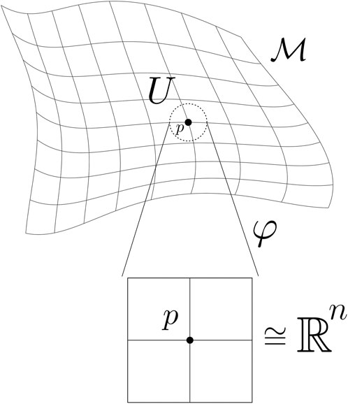
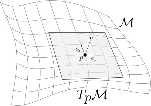
In [67], a two-dimensional vector space of the extensive area variables $(A_w,A_n)$ was studied, and the terminology of manifolds was left out. The idea here is similar, but we instead define the space of extensive areas to be a two-dimensional manifold where $(A_w,A_n)$ is a possible set of coordinates labeling a point on the manifold; see Figure 4. We label this manifold by $\mathcal{M}$. Because we have from Equation 16 that $A_p$ is a dependent variable, we only need two independent extensive variables as coordinates on $\mathcal{M}$. We choose them to be $A_w$ and $A_n$, and the assignment of the coordinates $\left(A_w,A_n\right)\in {\mathbb{R}}^2$ to an abstract point $p\in \mathcal{M}$ is formally done by a map $\phi$.⁵. The tangent space at each point of $\mathcal{M}$, which is simply the space of all tangent vectors that have this point as their initial point or origin, has a vector space structure by definition; see Figure 5. Intuitively, this is a vector space of the “linear approximations” of paths in the manifold, one space for each point in $\mathcal{M}$. In other words, at each point of $\mathcal{M}$, the tangent space is a space of possible directions in $\mathcal{M}$. We will describe these directions in terms of partial derivative operators, which is quite common due to its simple description in terms of coordinates [71].

Figure 4

Figure 4. The chart $\varphi$ is a (smooth) map from a neighborhood $U$ of a point $p$ on the general manifold $\mathcal{M}$ to an open subset of ${\mathbb{R}}^n$. Here, $\mathcal{M}$ is illustrated as a surface embedded in ${\mathbb{R}}^3$; however, the definition of a manifold is, strictly speaking, independent of embedding into larger, ambient spaces. The way this is depicted in the figure is thus only for the purpose of illustration.

Figure 5

Figure 5. The tangent space $T_p\mathcal{M}$ at a point $p\in \mathcal{M}$ can be imagined as a plane (strictly speaking, a vector space) attached to $\mathcal{M}$ at the point $p$. A tangent vector $v\in T_p\mathcal{M}$ can be imagined as a “small arrow” tangent to the manifold. The tangent vector $v$ can be expressed in some basis, for instance, $\left({\mathbf{e}}_1,{\mathbf{e}}_2\right)$.

In Figures 4, 5, the manifold is illustrated with curvature and embedded into ${\mathbb{R}}^3$. However, the definition of a manifold does not necessitate a larger space to embed the manifold in, and structure-like curvature could be intrinsic to the manifold itself. Such an additional structure could also be envisioned in our case. However, in this work, we only consider a neighborhood $U$ of a point $p\in \mathcal{M}$ isomorphic to a neighborhood of ${\mathbb{R}}^2$.⁶, meaning we only work in a patch ${\mathbb{R}}^2$ (see Figure 4) and disregard any additional structure of $\mathcal{M}$.⁷.

Because our space of extensive variables is now simply ${\mathbb{R}}^2$, it might seem unnecessary to separate the manifold from its tangent space. However, we cannot come to any of the conclusions in this work if we do not formally keep them separate. The motivation here for introducing a manifold and its tangent spaces is to be able to formally discern extensive and intensive variables. This is necessary to explain why our theory acts like a thermodynamic theory. As mentioned earlier, the vector spaces in [67] did not separate between the space of extensive variables and that of velocities; areas and velocities were simply elements of the same vector space. In a geometrical approach to physics, one often separates the two by means of a bundle structure⁸, with a base manifold acting as a configuration space and some space of objects attached to each point of the configuration space. The geometry of classical mechanics as a whole is based on this structure, and geometric descriptions of thermodynamics use exactly the same framework. For instance, what we call “extensive” and “intensive” variables in thermodynamics are examples of canonical coordinates [72], the coordinates on the “thermodynamic phase space” analogous to the phase space of positions and momenta in Hamiltonian mechanics. Without a clear distinction between the two types of variables, one would not be able to introduce geometric structures that define thermodynamic equilibrium states, Legendre-manifolds [72], or talk about metrics on the thermodynamic phase space, which connects thermodynamics to statistical mechanics [73]. Thus, separating the extensive and intensive variables in the same way as in geometrical physics is a natural step in a “geometrization” of the theory in this work.

3.1 Tangent space, bundle, and frames

We introduce the tangent bundle structure to formally distinguish extensive variables and velocities. A tangent bundle is intuitively simply a base space (here, a configuration space) together with the space of possible “directions” at each point of this space. The meaning of “direction” can be made more precise in several equivalent ways [74]. Here, we apply the perhaps most common one by identifying directions with partial derivative operators, which gives the most straightforward relations in the current context. These operators act on functions defined on the base space, of which $Q$ is an example. The point is to make a separation into two types of variables and encode the fact that all information about the system should be captured in the function $Q$.⁹.

Consider at every point $p\in \mathcal{M}$ the tangent space $T_p\mathcal{M}$ at that point; see Figure 5. The collection of all such tangent spaces of $\mathcal{M}$ along with their points of attachments is a manifold called a tangent bundle [74]¹⁰. We denote the total space of the tangent bundle of $\mathcal{M}$ by $T\mathcal{M}$. An element of the tangent bundle $T\mathcal{M}$ is a pair $\left(p,u\right)$, where $p\in \mathcal{M}$ is the point of attachment of the tangent space on $\mathcal{M}$, together with a tangent vector $u\in T_p\mathcal{M}$. We can express $p$ in coordinates as, for example, $p=(A_w,A_n)$, and $u$ can be expressed via the components $(u_1,u_2)$ of the vector $u$ expressed in some vector space basis of $T_p\mathcal{M}$. With the bundle structure follows the projection $\pi :T\mathcal{M}\to \mathcal{M}$. For each $(p,u)$, $\pi$ is simply the projection onto the base point $p$; that is, we “forget” about the vector $u$.

Because $\mathcal{M}\cong {\mathbb{R}}^2$, we have that for each $p\in \mathcal{M}$ that $T_p\mathcal{M}\cong T_p{\mathbb{R}}^2\cong {\mathbb{R}}^2$, and that $T\mathcal{M}\cong T{\mathbb{R}}^2\cong {\mathbb{R}}^2\times {\mathbb{R}}^2$. This means that $\mathrm{d}\mathrm{i}\mathrm{m}\left(T\mathcal{M}\right)=4$.

Consider now a general tangent vector field $V$ on $\mathcal{M}$, also called a section of the bundle $T\mathcal{M}$. $V$ is a map $V:\mathcal{M}\mapsto T\mathcal{M}$, a choice of a vector $V_p\in T_p\mathcal{M}$ at every point $p\in \mathcal{M}$. We are here assuming that this choice of vector at each point is smooth in the sense that the vector components are smooth functions on the manifold. Let ${\mathbf{v}}_i$ be a basis of the tangent space $T_p\mathcal{M}$. We will use a bold font on general basis vectors to separate them from their coordinates. We can, as usual, expand any tangent vector $V_p$, $p\in \mathcal{M}$, in the basis ${\mathbf{v}}_i$ as Equation 38:

$V_p=v^i\left(p\right){\mathbf{v}}_i,(38)$

where $v^i$ are the coordinates of $V_p$ with respect to ${\mathbf{v}}_i$, which are functions of $p$. We use the Einstein summation convention here and onward. Similarly, we can expand a vector field $V$ using a set of sections ${\mathbf{s}}_i$ as

$V=f^i{\mathbf{s}}_i,(39)$

where $f^i$ are functions on $\mathcal{M}$.

We adopt the common convention that the basis of tangent vectors at a point $p\in \mathcal{M}$ are directional derivatives acting on smooth functions on the base space at that point [71, 74]. A chart on some open set $U\subset \mathcal{M}$ containing the point $p$, given, for example, by coordinate (functions) $x^i(p)\equiv \left(A_w,A_n\right)$, gives a natural basis for the tangent space $T_p\mathcal{M}$: the partial derivatives with respect to the coordinate functions $x^i$ viewed as “attached” at $p$.

Equation 40 introduces the notation

${\left\{{\left.\frac{\partial }{\partial x^i}\right|}_p\right\}}_{i=1}^n\equiv {\left\{{\left.{\partial }_{x^i}\right|}_p\right\}}_{i=1}^n,(40)$

where $n$ is the dimension of the manifold. In the case of $p=(A_w,A_n)\in \mathcal{M}$, we then have that

$\left\{\frac{\partial }{\partial A_w},\frac{\partial }{\partial A_n}\right\}\equiv \left\{{\partial }_w,{\partial }_n\right\}(41)$

is a basis for the tangent space at each point $p$. The partial derivatives act on smooth functions $f:\mathcal{M}\to \mathbb{R}$, which are simply functions that take points on the manifold $\mathcal{M}$ as input. The total volumetric flow rate $Q=Q\left(A_w,A_n\right)$ is such a function.

We can now identify the thermodynamic velocities (Equation 28, 29) as being the basis $\left({\partial }_w,{\partial }_n\right)$ acting on the function $Q$; we have “decoupled” the vectors from the functions on which they act. The partial derivatives with respect to $A_w$ and $A_n$ at a point $p$, denoted by ${\partial }_w{|}_p$ and ${\partial }_n{|}_p$, respectively, acting on the volumetric flow rate $Q$ define the thermodynamic velocities. We have such a derivation at each point $p\in \mathcal{M}$, so we can view $\left\{{\partial }_w,{\partial }_n\right\}$ as coordinate vector fields on $\mathcal{M}$. These correspond to the sections ${\mathbf{s}}_i$ in Equation 39. In the same way, from now on, we identify any velocity with some tangent vector acting on $Q$. For instance, the pore velocity function $v$ can be identified with a tangent vector field that has components $\left(S_w,S_n\right)$ in the basis $\left\{{\partial }_w,{\partial }_n\right\}$, that is $S_w{\partial }_w+S_n{\partial }_n$. Upon acting on $Q$, we get the pore velocity function $v$.

In the same way, we view the seepage velocities $v_i$ as being defined by derivations acting on $Q$. In other words, we say that there exists a basis ${\mathbf{e}}_i$ of the tangent spaces of $\mathcal{M}$ that yield the seepage velocities upon acting on $Q$,

${\mathbf{e}}_i\left(Q\right)\equiv v_i,(42)$

where $i=w,n$. The basis ${\mathbf{e}}_i$ is strictly speaking a frame, which means that the frame elements ${\mathbf{e}}_i$ could be linearly dependent.

In the following, we will use the notation $v$, ${\widehat{v}}_w$, $v_n$, etc., to signify the velocity functions and use the notation $V$, ${\partial }_i$ and ${\mathbf{e}}_i$ for the vector fields associated with the velocity functions.

Note, in particular, that Equation 26 can be written as the action of a tangent vector field on $Q$, which acts as the identity. We have a vector field $\mathrm{\Delta }$ acting like Equation 43:

$\mathrm{\Delta }\left(Q\right)=A^i{\partial }_i\left(Q\right)=A_w{\left(\frac{\partial Q}{\partial A_w}\right)}_{A_n}+A_n{\left(\frac{\partial Q}{\partial A_n}\right)}_{A_w},(43)$

which by Equation 26 is equal to $Q$ through the Euler theorem. Strictly speaking, we should be more careful with the notation: $A_w$ and $A_n$ as prefactors to ${\partial }_w$ and ${\partial }_n$ are here coordinates on the “fiber,” the tangent space. This means that they are simply the components of a vector. Meanwhile, $A_w$, $A_n$ in ${\partial }_w$ and ${\partial }_n$ are the coordinate functions on $\mathcal{M}$. We will not encounter problems by not distinguishing them in this work, so we keep the notation as is for simplicity.

We have in this section shown how the velocities in Section 2 can be interpreted as objects on a tangent bundle with base space $\mathcal{M}$. When these tangent vectors act on the function $Q$, we obtain the ordinary velocity functions, which give a number for each $p\in \mathcal{M}$. This simple fact is the link to the “classical” geometric viewpoint we alluded to in Section 1. In what follows, we will use this relation with ordinary numbers and motivate the introduction of affine spaces from the definition of the pore velocity $v$. We will then use the fact that we can relate tangent vectors to points of an affine space (the tangent vector spaces are actually affine spaces over themselves) and show how this is helpful in the geometric interpretation presented in this work.

3.2 Affine spaces of velocities, displacement, and tangent vectors

The idea presented in the previous section applies differential operators to define fields corresponding to the velocities, which acted on $Q$ to produce the velocity functions. This type of separation is well suited for generalization to more high-level frameworks and has been considered by other authors in the context of thermodynamics (see, e.g., [70]). However, the relations in Section 2 can be interpreted more straightforwardly in terms of classical affine geometry. In this section, we show how this can be done, noting that this does not exclude the differential geometric viewpoint: the classical picture is here possible due to the identification $\mathcal{M}\cong {\mathbb{R}}^2$. The reason one might use this framework instead of a differential geometric one is that it provides a more intuitive picture in terms of configurations of points and lines that can be visualized more easily. Moreover, it is closely related to constitutive relations like Equation 14 because these relations are framed in terms of functions and not algebraic objects like vector fields. This view could potentially be useful in obtaining new constitutive relations for $v_m$ in the future.

First, we will show explicitly how classical affine geometry enters the problem. Let the tangent vectors introduced in the previous section act on $Q$, such that we obtain the ordinary velocity functions. By the map given in Equations 32, 33, we can rewrite the definition of the pore velocity function $v$, Equation 30, as

$v=S_w{\widehat{v}}_w+S_n{\widehat{v}}_n=v_m+S_w\left({\widehat{v}}_w-v_m\right)+S_n\left({\widehat{v}}_n-v_m\right).(44)$

If we were to treat the velocities themselves as points in some abstract space and then apply our intuition from Euclidean spaces where the difference between two points corresponds to a vector, Equation 44 is exactly a vector (a linear combination with $S_w,S_n$ as coefficients) “attached” at the point $v_m$. In this section, we will make this idea more formal through affine spaces. The differences between the differential-geometric and the affine descriptions presented in previous sections will be elucidated, and the necessary concepts for analyzing the co-moving velocity $v_m$ in terms of affine maps will be given in Section 4.

Formally, an affine space [75] is a set $\mathcal{A}$ of points together with a vector space $\overrightarrow{\mathcal{A}}$, equipped with a map $\mathcal{A}\times \overrightarrow{\mathcal{A}}$$\to \mathcal{A}$. This map can be said to be the action of a vector $v\in \overrightarrow{\mathcal{A}}$ on a point $p\in \mathcal{A}$, acting as a displacement to another point $p^{\prime }\in \mathcal{A}$. The “difference” between two points $p,p^{\prime }\in \mathcal{A}$ can be identified with an element $v\in \overrightarrow{\mathcal{A}}$, which intuitively mean that the difference between two points can be identified with the vector between them. We then have a space $\mathcal{A}$ of points, and a space $\overrightarrow{\mathcal{A}}$ of all displacements between points of $\mathcal{A}$.

Coordinates on affine spaces entail a choice of an origin (a “zero vector”) and a linear basis with respect to this origin. Consider an affine space $\mathcal{A}$ of dimension $n$, and let $o\in \mathcal{A}$ be a choice of origin. Let $\left({\mathbf{e}}_1,{\mathbf{e}}_2,\dots ,{\mathbf{e}}_n\right)\equiv \left\{{\mathbf{e}}_i\right\}$ be a choice of basis of $\overrightarrow{\mathcal{A}}$. Then, any point $p\in \mathcal{A}$ can be written as

$p=o+\left(p-o\right)=o+p^i{\mathbf{e}}_i,(45)$

where $\left(p-o\right)$ is a vector because it is the difference between two points, which we on the second line of Equation 45 expanded in the basis ${\mathbf{e}}_i$ with components $\left\{p^i\right\}$. The components $\left\{p^i\right\}$ are the affine coordinates of the point $p$. A new choice of origin $o$ or basis $\left\{{\mathbf{e}}_i\right\}$ specifies a new set of affine coordinates. The choice of an origin and a linear basis with respect to this origin is an affine frame or affine basis.

An affine map $f$ is a map between affine spaces that preserves the affine structure. Any such map $f:\mathcal{A}\to \mathcal{B}$ between affine spaces $\mathcal{A}$, $\mathcal{B}$, with associated vector spaces $\overrightarrow{\mathcal{A}}$ and $\overrightarrow{\mathcal{B}}$, respectively, is defined by the property that for any two points $a,b\in \mathcal{A}$, we have

$f\left(a\right)-f\left(b\right)=\lambda \left(a-b\right),(46)$

where $\lambda$ is a linear map. Expressed equivalently, we have Equation 47,

$f\left(p+u\right)=f\left(p\right)+\lambda u,(47)$

where $p\in \mathcal{A}$ is a point, $u\in \overrightarrow{\mathcal{A}}$ is a vector, and $\lambda$ is a linear map. By fixing points $o_1\in \mathcal{A}$, and $o_2\in \mathcal{B}$, a general affine map $f:\mathcal{A}\to \mathcal{B}$ can be written in the form

$f\left(p\right)=o_2+\left(f\left(o_1\right)-o_2\right)+\lambda \left(p-o_1\right),(48)$

for $p\in \mathcal{A}$. Here, $\left(f(o_1)-o_2\right)$ is a translation of $\mathcal{B}$ which only depends on $o_1$ and $o_2$, and $\lambda (p-o_1)$ is a linear map of the vector $\left(p-o_1\right)\in \overrightarrow{\mathcal{A}}$. At any point, we can form a vector space and define some basis with respect to this point. We can, for instance, take the derivative operators discussed in Section 3.1 as a basis for the vector space at this point. In this work, we can identify it with the tangent space at that point. Thus, the vector $\lambda \left(p-o_1\right)$ can be treated as a tangent vector attached at $o_1$, obtained in coordinates by specifying affine coordinates for the point $p$. A very important point is that by Equation 48, a translation of the origin is also given by a vector or, equivalently, a tangent vector in this case.

A special case of an affine map is an invertible affine map from an affine space $\mathcal{A}$ to itself, $f:\mathcal{A}\to \mathcal{A}$. Such a map is an affine transformation of $\mathcal{A}$ and satisfies Equation 49:

$f\left(p\right)=o+\left(f\left(o\right)-o\right)+\lambda \left(p-o\right)(49)$

with $p\in \mathcal{A}$ and $o\in \mathcal{A}$ is taken as the origin, and $(f(o)-o)$ is a translation.

For an affine combination of points $\left\{e_i\right\}$ with coefficients ${\alpha }_i$, an affine map $f$ satisfies

$f\left({\displaystyle \sum _{i=1}^n}{\alpha }_i{e}_i\right)={\displaystyle \sum _{i=1}^n}{\alpha }_{i}f\left(e_i\right).(50)$

In terms of the concepts introduced in this section, one can see that Equation 44 expresses $v$ as an affine combination with $v_m$ singled out as a choice of origin. Thus, we interpret the velocities $v$, ${\widehat{v}}_i$, $v_i$, and $v_m$ as points of an affine space $\mathcal{A}$, with an associated vector space $\overrightarrow{\mathcal{A}}$ of displacements. We view the space of velocities as affine because $v_m$ determines a “moving origin,” $v_m=v_m\left(S_w\right)$.

Formally the velocities are points of $\mathcal{A}$,

$v,{\widehat{v}}_i,v_i,v_m\in \mathcal{A},(51)$

whereas the velocity differences $\left({\widehat{v}}_i-v_m\right)$ are not vectors in $\overrightarrow{\mathcal{A}}$. They are simply functions, giving a real number for each value of the saturation $S_w$.

In terms of symmetry groups of affine spaces, affine transformations of these spaces are said to act transitively. Consider two pairs of points, such as the thermodynamic velocities $\left({\widehat{v}}_w,{\widehat{v}}_n\right)$ and the seepage velocities $\left(v_w,v_n\right)$ in $\mathcal{A}$. If we have a map $g\in G$ for some group $G$ such that $g\left({\widehat{v}}_w,{\widehat{v}}_n\right)=\left(v_w,v_n\right)$, the group $G$ is said to act 2-transitively on $\mathcal{A}$. The map $f$ in Equation 56 is exactly such a 2-transitive map. That $f$ acts 2-transitively of $\left({\widehat{v}}_w,{\widehat{v}}_n\right)$ means that if we know how one velocity is mapped, the map of the other is known. This is exactly what is described by the relation defined in Equations 32, 33. A concrete example of a group of affine transformations is the group consisting of translations and homotheties, or the group of dilations [76]. We will apply these transformations in a practical example of a capillary fiber bundle model in Section 4.2.

We now stress an important point regarding the relation between the “classical” and differential-geometric descriptions: the vector space of displacements $\overrightarrow{\mathcal{A}}$ and the tangent vector spaces $T_p\mathcal{M}$ at each point $p\in \mathcal{M}$ are formally not the same spaces. However, they are isomorphic in the case of $\mathcal{M}\cong {\mathbb{R}}^2$. The tangent spaces at each point of $\mathcal{M}$ can, in the case where we regard the underlying space to be simply $\mathcal{M}\cong {\mathbb{R}}^n$, be identified with each other by translations. This is not possible in general; for a general manifold, each tangent space must be viewed as distinct, as the concept of simple displacements needs amending [75]. We note that in the infinitesimal (tangent vector) case, the co-moving velocity $v_m$ is, in general, an example of a particular type of section of a bundle; see Section 5.2.

In Section 3.1, we defined the tangent vector spaces $T_p\mathcal{M}$, $p\in \mathcal{M}$, without endowing $\mathcal{M}$ itself with any particular structure. In fact, we could view $\mathcal{M}$ itself as an affine space. As an example of why this might be useful, consider the case where we have some constant irreducible saturation in the two-phase flow system. If the irreducible saturation is associated with some constant non-vanishing flow rate, we have a constant term in our description of the areas and the velocities that we must take into account. The problem can then be simplified if one could specify a new convenient origin in $\mathcal{M}$, for instance, one corresponding to the irreducible saturation.

Therefore, we have seen that it can be useful to view $\mathcal{M}$ as not having a fixed origin $O$. The latter was considered in [67]. By specifying some origin $O$, one obtains a vector space structure. On the other hand, in order to refer to the relation between the choices of origins, one needs the affine structure. It turns out that in the case where we take the base space $\mathcal{M}$ to itself be an affine space, we can identify the tangent spaces at different points of $\mathcal{M}$ by translations of $\mathcal{M}$: given some vector $u$, one can consider the translation or displacement ${\tau }_u:\mathcal{M}\to \mathcal{M}$ of all points of the affine space $\mathcal{M}$ by this vector [76]. Note that this is a translation of all points of the space $\mathcal{M}$ and does not act as a derivation at a point as in the case of tangent vectors. These translations are elements of the vector space associated to $\mathcal{M}$ viewed as an affine space.

Let this associated vector space to $\mathcal{M}$ be denoted by $\overrightarrow{\mathcal{M}}$. We note that $\overrightarrow{\mathcal{M}}$ can be identified with the “vector space of areas” from earlier work [67]. The vector space $\overrightarrow{\mathcal{M}}$ associated to the affine space $\mathcal{M}$ can be viewed as containing the displacements between points of $\mathcal{M}$, simply as with $\mathcal{A}$ and $\overrightarrow{\mathcal{A}}$ from earlier in this section. A tangent vector $u\in T_p\mathcal{M}$ can be regarded as a tangent vector to a curve (which we take to be only a line) $t\mapsto p+tu$ at the point $p\in \mathcal{M}$ [75]. Any displacement vector $u^{\prime }\in \overrightarrow{\mathcal{M}}$ with the same direction as $u$ would give the same curve. If we consider the limit where the displacement given by $u^{\prime }$ goes to zero, we see that we naturally have that we can let $u\in \overrightarrow{\mathcal{M}}$. Thus, we can view the tangent space at each point $p\in \mathcal{M}$ as a copy of $\overrightarrow{\mathcal{M}}$ attached to $p$. This identification between vectors of $\overrightarrow{\mathcal{M}}$ and vectors in $T_p\mathcal{M}$ at each $p\in \mathcal{M}$ is only possible due to the affine structure of $\mathcal{M}$, and it is important to note that this does not hold for general manifolds. This is so because there is, in general, no natural way of identifying vectors at different points of a manifold without introducing a connection on the bundle [71, 77]. Such a connection is extraneous to the manifold itself. Note that the difference between the two is that the elements of $\overrightarrow{\mathcal{M}}$ are, intuitively, “detached” from any point $p$.

To sum up, we only need a single space $\mathcal{M}$, whose displacements live in the vector space $\overrightarrow{\mathcal{M}}$. We can either use the tangent vectors at each point to describe the velocities at each point $p\in \mathcal{M}$, or we can let these tangent vectors act on $Q$ and instead use the (signed) distances between points of $\mathcal{M}$ as representing the displacements. This correspondence is possible due to the identification $\mathcal{M}\cong {\mathbb{R}}^2$. In the latter case, we essentially do not use the manifold structure of $\mathcal{M}$ and only treat it as the linear space ${\mathbb{R}}^2$.

3.3 The saturation as a coordinate and parameter

In the description of velocities as points in an affine space, Equation 51, we have an important relation for the space $\mathcal{M}$ of extensive variables: we can use the velocities to identify “directions” in $\mathcal{M}$. More explicitly, ratios of distances (the “lengths” of the vectors in $\overrightarrow{\mathcal{M}}$) can be identified with points on an affine line $L\subset \mathcal{M}$ through their functional values. We can specify points on this line either by specifying a value of $S_w$, or by specifying the values of the velocity differences. We will now clarify this point.

The specific coordinates on $\mathcal{M}$ do not really matter [67], so we specify points $p\in \mathcal{M}$ using the extensive areas, $p=\left(A_w,A_n\right)\in \mathcal{M}$. However, for practical reasons, it is often convenient to work with the coordinates [50] $(S_w,A_p)$, defined by

$A_p\equiv A_w+A_n,(52)$

$S_w\equiv \frac{A_w}{A_w+A_n}=\frac{A_w}{A_p}.(53)$

If we view $A_p$ as fixed and constant, we only have a single variable $S_w$. For each constant value $A_p=A_p^{*}$, $S_w$ parametrizes a line $L\subset \mathcal{M}$ running between $(A_w,A_n)=(0,A_p^{*})$ and $(A_p^{*},0)$. In these coordinates $\left(A_w,A_n\right)$, we have the “trivial” parametrization $\left(S_w{A}_p^{*},\left(1-S_w\right)A_p^{*}\right)$.

Because $\mathcal{M}\cong {\mathbb{R}}^2$, each $L$ (one for each value of $A_p^{*}$) can be seen as an affine subspace of $\mathcal{M}$ In terms of manifolds, $L$ is a sub-manifold of $\mathcal{M}$. The use of the term “affine subspace” in this case is only due to our identification of $\mathcal{M}$ with the real plane ${\mathbb{R}}^2$, viewed as a vector space itself. $S_w$ is, in this context, called an affine coordinate on the line $L$. Moreover, $S_w$ is a parameter that specifies a point on the line $L$ defined by $A_w+A_n-A_p^{*}=0$.

The velocity functions are equivalent to one-dimensional maps of the parameter $S_w$, which, for example, sends $S_w\mapsto {\widehat{v}}_w\left(S_w\right)\in L$. The relation between $S_w$ and the velocities are obtained by solving Equation 31 for $S_w$, finding

$S_w=\frac{v-{\widehat{v}}_n}{{\widehat{v}}_w-{\widehat{v}}_n}=\frac{v-v_n}{v_w-v_n}(54)$

where the velocity differences are simply the values of the corresponding functions. Thus, $S_w$ give the position of $v$ on the line segment with ${\widehat{v}}_w$ and ${\widehat{v}}_n$ or $v_w$ and $v_n$ as endpoints for $v$.

The view of $S_w$ as a parameter specifying a point on the line $L$ is quite useful for concrete computations. In fact, instead of letting $A_p$ equal a constant $A_p^{*}$, we can consider all relations “modulo” the scale factor $A_p$, and work with the parameter $S_w$ alone. By this, we mean that transformations in the parameter $S_w$ are related to a (potentially continuous) family of lines $\left\{L_i\right\}$ in $\mathcal{M}$, where each line $L_i$ is given by a linear inhomogeneous equation $a{A}_w+b{A}_n=c$, where $a$, $b$, and $c$ are constants. This serves as the entry point for continued work on the affine-geometric interpretation of the system and connects the affine relations in this work to projective geometry [76, 78]. In this context, where we can specify points on a line $L$ by using the “dual” intensive quantities to the extensive variables, the velocities $\left\{v,{\widehat{v}}_w,{\widehat{v}}_n\right\}$, or equivalently $\left\{v,v_w,v_n\right\}$, can be called a type of projective basis or projective frame [78, 79]. A map of the velocities sending ${\widehat{v}}_i\mapsto v_i$ can, in this context, be said to be a map defined on the dual space of $\mathcal{M}$. What is meant by “dual” depends on the context, but in this specific case, one is referring to the projective dual of $\mathcal{M}$, denoted ${\mathcal{M}}^{*}$. This is simply the space where each point $a\in {\mathcal{M}}^{*}$ represents a line in $\mathcal{M}$. The velocities can then be seen as elements of ${\mathcal{M}}^{*}$ because they exactly specify lines in $\mathcal{M}$. This can be seen by writing Equation 31 as

$\begin{array}{c}{A}_w\left({\widehat{v}}_w-v\right)+A_n\left({\widehat{v}}_n-v\right)=A_w\left(v_w-v\right)+A_n\left(v_n-v\right)=0.\hfill \end{array}(55)$

In Equation 55, $\left(A_w,A_n\right)$ specifies points of $\mathcal{M}$, while the (ratio of the) velocities give the slope of the line through the point $\left(A_w,A_n\right)$. In the special case that $\mathcal{M}\cong {\mathbb{R}}^2$, this duality is trivial; however, this is the formal relation between the extensive and intensive variables in the affine viewpoint. We will not need more specifics about these spaces and reserve this for future work.

4 The co-moving velocity and affine maps

We will now investigate how the co-moving velocity $v_m$, first presented in Equation 13, can be described in terms of the two views of the velocities presented in previous sections. As already mentioned in Section 3.2, we have a natural identification between the tangent spaces at each point of $\mathcal{M}$ and the vector space $\overrightarrow{\mathcal{M}}$ of displacements of points of $\mathcal{M}$. From the discussion in the preceding sections, we can work with either the distances between points given by the differences $\left(v_i-v_m\right)$, or with tangent vectors at each point. We will start by using the former description, where it is implicit that we have restricted ourselves to a line $L\subset \mathcal{M}$ such that $S_w$ is a parameter along $L$, as discussed in the previous section. We will then use the tangent vector description to write the relations in terms of vector components before simplifying the obtained relations. The result will, in the two cases, be an expression for a function of $v^{\prime }=dv/d{S}_w$ and a vector field corresponding to the co-moving velocity $v_m$, respectively.

4.1 $v_m$ from affine maps

Let $f$ be an affine map. We now apply the general property in Equation 50 of these maps to show how the linear term in Equation 14 can be obtained. Comparing with Equation 31, we see that the mapping $\left\{{\widehat{v}}_i\right\}\mapsto \left\{v_i\right\}$, which we define to be given by our map $f$, by definition should satisfy

$\begin{array}{ll}\hfill v=f\left(v\right)& =f\left(S_w{\widehat{v}}_w+S_n{\widehat{v}}_n\right)\hfill \\ \hfill & =S_{w}f\left({\widehat{v}}_w\right)+S_{n}f\left({\widehat{v}}_n\right)\hfill \\ \hfill & =S_w{v}_w+S_n{v}_n,\hfill \end{array}(56)$

which holds because $S_w+S_n=1$ at all times. Thus, $f$ can be seen as an affine map $f:{\widehat{v}}_i\mapsto v_i$ leaving the convex combination $v$ invariant.

The details about the map $f$ depend on which interpretation we have for the velocities. As expressed in the discussion around Equation 56, $f$ as a map of the velocities is formally a map on ${\mathcal{M}}^{*}$, the space of lines in $\mathcal{M}$. However, because we can simply view the velocities as functions of $S_w$ only, $f$ is simply a map of the one-dimensional number line $\mathbb{R}$. It is not important if this number line is embedded in some higher dimensional space. We will call this line $l$, the image of $S_w\in L$ under the velocity functions. This is what we will take as the meaning of the map $f$ of the velocities: as a map of their functional values on the line $l$. We will return to the case of $f$ acting on tangent vectors, where the idea is exactly the same but expressed differently.

With the notion of an affine map $f$, we can revisit the right-hand side of Equation 44. The velocities $\left({\widehat{v}}_n+S_n{v}_m\right)$, $\left({\widehat{v}}_n+S_w{v}_m\right)$ are in this case not velocity differences; they are expressions of a particular affine map called a homothety; see Section 4.2. In fact, $v$ itself can be written as a homothety. To see this, we rewrite Equation 31 as

$v={\widehat{v}}_w+S_n\left({\widehat{v}}_n-{\widehat{v}}_w\right)=v_w+S_n\left(v_n-v_w\right),(57)$

where the middle and third expressions, respectively, are homotheties of ratio $S_n$ with centers $v_w$ and ${\widehat{v}}_w$ [76].

Consider $\left\{{\widehat{v}}_i\right\}$ and $\left\{v_i\right\}$ as points in two affine spaces $\mathcal{A}$, $\mathcal{B}$ with associated vector spaces $\overrightarrow{\mathcal{A}}$ and $\overrightarrow{\mathcal{B}}$, respectively. Using Equation 34 and Equation 56, we have that

$\begin{array}{ll}\hfill f\left({\widehat{v}}_w\right)-f\left({\widehat{v}}_n\right)& =v_w-v_n\hfill \\ \hfill & =\frac{dv}{d{S}_w}-v_m.\hfill \end{array}(58)$

The velocity difference $(v_w-v_n)$, where $v_i=f({\widehat{v}}_i)$, is then equivalent to a linear map $\lambda$ of $\left({\widehat{v}}_w-{\widehat{v}}_n\right)$ according to Section 3.2. In writing, $\left(f({\widehat{v}}_w)-f({\widehat{v}}_n)\right)=(v_w-v_n)$, we can specify a choice of origin in $\mathcal{A}$ and $\mathcal{B}$. We choose the origins $o\in \mathcal{A}$ and $p\in \mathcal{B}$, and use Equation 48 and Equation 58 to write Equation 59,

$f\left({\widehat{v}}_w\right)=f\left({\widehat{v}}_n\right)+\lambda \left({\widehat{v}}_w-{\widehat{v}}_n\right),(59)$

which from Section 3.2 is equivalent to

$\begin{array}{ll}\hfill f\left(o+u\right)& =p+\left(f\left(o\right)-p\right)+\lambda u\hfill \\ \hfill & =p+\lambda u,\hfill \end{array}(60)$

for some vector $u$, and where we let $f(o)\equiv p$. We can then set $f\left(o+u\right)=f\left({\widehat{v}}_w\right)$, the new origin $p=f\left({\widehat{v}}_n\right)$, $\lambda u=\left(v^{\prime }-v_m\right)$. The point is that the affine map $f$ also moves the origins of the velocities.

As before, we can associate the vector $u$ with its (Euclidean) length of the distance between points on the line $l$. Thus, the meaning of Equation 60 is simply that a velocity defined by the distance $u$ from some origin $o$ is mapped to a new origin $p$ and a linear map of the distance $u$. Even if we a priori have no preferred way of defining such an origin or vector $u$, the map $f$ suggests that the origin should move, and the distance $u$ from the origin is scaled by $\lambda$.

We are now ready for a simple yet important result. Comparing Equation 58 to the definition in Equation 46, we see that we can write

$\begin{array}{ll}\hfill f\left({\widehat{v}}_w\right)-f\left({\widehat{v}}_n\right)& =\lambda \left({\widehat{v}}_w-{\widehat{v}}_n\right)\hfill \\ \hfill & =\lambda \left(v^{\prime }\right)=v^{\prime }-v_m,\hfill \end{array}(61)$

where $\lambda$ is a linear map. In one dimension, the only linear maps are multiplication by a scalar, so $\lambda$ is only a number. Thus, we have

$v_{m,\mathcal{A}}=\left(1-\lambda \right)v^{\prime },(62)$

where the subscript $\mathcal{A}$ is included simply to stress that this result is the one obtained from the affine relations in this section¹¹. We will see that we get a similar form in Equation 62 when treating the velocities as tangent vector fields in Section 4.3.

4.2 Homotheties and irreducible capillary flow

Intuitively, Equation 57 means that $v$ is the point located at a fraction $S_n$ along the line segment between ${\widehat{v}}_w$ and ${\widehat{v}}_n$ in $\mathcal{A}$. Thus, if either ${\widehat{v}}_w$ or ${\widehat{v}}_n$ (or both) were to change while $v$ was kept fixed, $S_n$ would also change, and hence also $S_w=1-S_n$. Thus, any change in one of the thermodynamic velocities is accompanied by an equal and opposite change in the other thermodynamic velocities. This is the relation between the middle and last expressions in Equation 57 and also in Equation 56. In fact, affine maps are the only maps that “commute” with the saturation $S_n$ in this way, which we see is the defining property, which we use to introduce $v_m$ through Equations 32, 33.

We will now use two particular affine maps, a translation and a homothety, to demonstrate that even though the maps between the seepage and thermodynamic velocities can be modeled as affine, endowing both the space of velocities and extensive variables with this structure allows for considering more complicated expressions for $v_m$. We here use an example of a capillary fiber bundle with two types of capillaries, considered in earlier works on $v_m$ [50]. This will show that the derivation of $v_m$ can be expressed in terms of affine maps in a rather straightforward manner.

Let ${\tau }_u$ be a translation of $\mathcal{A}$ by the vector $u$, and let $h_{s,\lambda }$ be a homothety of center $s$ and ratio $\lambda$. Intuitively, ${\tau }_u$ simply translates all points $x$ in $\mathcal{A}$ to the points $u+x$, while $h_{s,\lambda }$ scales all vectors $\overrightarrow{sx}$ for all points $x\in \mathcal{A}$ by a factor $\lambda$. Because the set of translations and homotheties of an affine space forms a group [76], a composition of ${\tau }_u$ and $h_{s,\lambda }$ is again a homothety ${\tilde{h}}_{\tilde{s},\lambda }$ of center $\tilde{s}$. Explicitly, if $h_{s,\lambda }:p\mapsto s+\lambda \left(p-s\right)$, and ${\tau }_u:p\mapsto p+u$ with $u$ a vector, we have

${\tau }_u◦h_{s,\lambda }:p\mapsto s+u+\lambda \left(p-s\right).(63)$

We can rewrite Equation 63 as a new homothety $\tilde{h}$ with respect to a point $\tilde{s}$ and the same ratio $\lambda$ as

${\tau }_u◦h_{s,\lambda }:p\mapsto s+\frac{u}{1-\lambda }+\lambda \left(p-\left(s+\frac{u}{1-\lambda }\right)\right).(64)$

If we define

$\tilde{s}=s+\frac{u}{1-\lambda },(65)$

we can define ${\tau }_u◦h_{s,\lambda }\equiv {\tilde{h}}_{\tilde{s},\lambda }$ and write Equation 64 as

${\tilde{h}}_{\tilde{s},\lambda }:p\mapsto \tilde{s}+\lambda \left(p-\tilde{s}\right).(66)$

The formalism in terms of homotheties, as defined above, can be applied directly to the system studied in Section 7.3 of [50]. This system consists of $N$ capillary fibers in parallel, of which $N_s$ have a smaller cross section $a_s$ and the rest, $N_l=N-N_s$, have a larger cross section $a_l$. We assume the smaller cross section is so small that only the wetting fluid can enter these capillaries. Each capillary is filled with either wetting or non-wetting fluid only. The wetting pore area is then $A_w=A_s+A_{lw}$ where $A_s=N_s{a}_s$ and $A_{lw}$ is the area of the large capillaries that are filled with wetting fluid. This means that the system has an irreducible saturation given by $S_{w,i}=A_s/A_p$. Hence, the wetting area is given by $A_w=A_p{S}_{w,i}+A_p\left(S_w-S_{w,i}\right)$. The non-wetting saturation is given by $S_n=1-S_w$. We denote the velocity of the non-wetting fluid by $v_n$, and the velocity of the wetting fluid in the small capillaries $v_{sw}$ and in the large capillaries by $v_{lw}$. The average flow velocities through the capillary fiber bundle are then

$v=S_{w,i}{v}_{sw}+\left(S_w-S_{w,i}\right)v_{lw}+S_n{v}_n.(67)$

We may now interpret the velocities as points in a space $\mathcal{A}$. We combine Equations 10, 67 to find

$S_w{v}_w=S_{w,i}{v}_{sw}+\left(S_w-S_{w,i}\right)v_{lw}.(68)$

We express $v_w$ by dividing the left-hand side of Equation 68 by $S_w$, and insert this into Equation 57 to obtain

$\begin{array}{ll}\hfill v& =v_w+S_n\left(v_n-v_w\right)\hfill \\ \hfill & =\left[v_{lw}+\frac{S_{w,i}}{S_w}\left(v_{sw}-v_{lw}\right)\right]\hfill \\ \hfill & +S_n\left[v_n-\left(v_{lw}+\frac{S_{w,i}}{S_w}\left(v_{sw}-v_{lw}\right)\right)\right]\hfill \\ \hfill & =v_{lw}+\frac{S_{w,i}}{1-S_n}\left(v_{sw}-v_{lw}\right)\hfill \\ \hfill & +S_n\left[v_n-\left(v_{lw}+\frac{S_{w,i}}{1-S_n}\left(v_{sw}-v_{lw}\right)\right)\right].\hfill \end{array}(69)$

Comparing Equation 69 to Equations 64, 65, we see that we have defined a composition of a homothety of ratio $S_n$ of the point $v_n$ with respect to the center $v_{lw}$ and the translation of the point $v_{lw}$ by the constant vector $S_{w,i}\left(v_{sw}-v_{lw}\right)$. We can thus identify it with a translation of the origin from $S_{w,i}{v}_{lw}$ to $S_{w,i}{v}_{sw}$. We may then rewrite Equation 69 one last time as

$v=v_{lw}-v_m+S_n\left(v_n-\left(v_{lw}-v_m\right)\right),(70)$

where we have identified

$v_m=\frac{S_{w,i}}{S_w}\left(v_{lw}-v_{sw}\right).(71)$

Comparing Equation 70 to Equation 66, we get that $\tilde{s}=v_{lw}-v_m$, meaning it can be viewed as a translation of the homothetic center $v_{lw}$. $v_m$ is exactly the translation vector of the homothetic center in the space of velocities.

We find from Equation 67 that

$v^{\prime }=\frac{dv}{d{S}_w}=v_{lw}-v_n.(72)$

Hence, $v_m$ in this system is not on the form suggested by Equation 62. The reason for this is that there is no mechanism in the capillary fiber bundle system to generate an equilibrium thermodynamics as the fibers are non-interacting.

We have in Section 4.1 related $v_m$ to the affine map $f$, with the result that Equation 62 is linear in $v^{\prime }$. Equation 61 means that $f$ acts the same way on both thermodynamic velocities. This restriction is what gives us Equation 62. When the constituent subsystems do not interact with each other as in the capillary fiber bundle example, which in general can happen in sub-regions of the saturation range, we see that we do not have a single map $f$ acting as in Equation 61. However, the velocity $v$ itself can be expressed in terms of a homothety, which is affine. This means that Equation 62 is not correct in this case. Solving Equation 71 for $v_{lw}$ and inserting into Equation 71 gives us Equation 73:

$v_m=\frac{S_{w,i}}{S_w}{v}^{\prime }+\frac{S_{w,i}}{S_w}\left(v_n-v_{sw}\right),(73)$

which contains a linear transformation in $v^{\prime }$.¹² and a translation term that moves the origin. In Section 5.2, we will see some solutions for describing this geometrically.

4.3 $v_m$ as a tangent vector field

We now turn to the interpretation of velocities as tangent vectors in the tangent spaces of $\mathcal{M}$, where $\mathcal{M}$ is again viewed as a manifold. We will exploit the fact that $\mathcal{M}\cong {\mathbb{R}}^2$ to circumvent a deeper discussion of connections (see Section 5.2 for a brief treatment) and mathematical fiber bundles. We will simply say that we are able to choose an origin $o$ in each tangent space that may depend on the point $p\in \mathcal{M}$. We regard vectors in the tangent space $T_p\mathcal{M}$ to be attached at the point $o\in T_p\mathcal{M}$. This origin is given by some section $s$ of $T\mathcal{M}$, which we assume to be non-vanishing for the domain in $\mathcal{M}$ we are considering. This means that the vector field itself has no singular points. A section of a bundle exists independently of a representation in terms of coordinates, so there is no intrinsic way of defining coordinates for a section unless more structure is provided.

We can encode an “indeterminate” origin in the tangent spaces of the bundle $T\mathcal{M}$ by letting the origin of the tangent spaces be given by a section $s_0$. This gives us an affine bundle [80], where the fibers are now related by affine maps. We cannot use the choice $s_0$ to define the coordinates of the section $s_0$ itself; the choice of $s_0$ is rather a part of the choice of affine frame generalized to the bundle (see Section 3.2), which allow us to define coordinates for vectors¹³.

In the following, we investigate what form of the co-moving velocity is permissible if we allow the thermodynamic and seepage velocities to be related by affine transformations in each tangent space. To do this, we must view each tangent space as an affine space. Intuitively, this means that we allow for picking an origin in each tangent space, with the restriction that this choice of origin must vary smoothly between neighboring tangent spaces. The tangent space at a point of a manifold is a vector space, while the affine tangent plane is any parallel translation of this tangent space. This complicates the matter because each of the linear structures of tangent spaces, as introduced in Section 3.1, is lost when we allow for such translations. One must then decide on how affine transformations are to be defined. We here outline two methods, one related to each of the two approaches in Section 3.1 and IIIB. We will use both of these in this section to obtain an expression analogous to Equation 62. This will serve to demonstrate how the differential and classical viewpoints are related.

The first method is to define an analog of a differential displacement vector, whose role is to translate the origin in each tangent space from 0 to the new origin, say $o$. In this way, one can work exclusively with vector fields. The consequence is that the components of the fields, the $f^i$ in Equation 39, acquire an extra term,

$f^i\mapsto {\bar{f}}^i+a^i,(74)$

where $a^i$ in general are functions of the base point, and ${\bar{f}}^i$ are the (linear) components of the vector fields. We will end up with field components in the form of Equation 74 later in this section.

The second way to work with this type of bundle structure is to keep the choice of origin in each tangent space, the zero section $s_0$, undetermined. This approach is equivalent in formulation to the formalism already introduced in Section IIIB. The vectors can then be viewed as “ordinary” Euclidean vectors (which we are unable to define explicitly because the origin is undetermined), while the points are viewed as formal objects subject to the rules of Section 3.2. In the end, only differences of points and vectors matter because the co-moving velocity is defined in terms of differences of points in Equations 32, 33. From Section 3.2, this means that we must only consider linear maps of the ensuing vectors. In the end, when we compute an analog of the co-moving velocity, a linear structure is therefore recovered. This will allow us to write a concrete expression for a vector field corresponding to $v_m$ in terms of coordinates at the end of this section. In the derivations below, we start out by describing the velocities as abstract points, which are decomposed into a general choice of origin and vector. We then end up considering linear transformations only when differences of points are computed.

Consider first a single tangent space $T_p\mathcal{M}$. Recall that $T_p\mathcal{M}$ is itself an affine space, denoted ${\mathcal{A}}_p$ with an associated vector space ${\overrightarrow{\mathcal{A}}}_p$. We consider the origin of ${\overrightarrow{\mathcal{A}}}_p$ as a point $\widehat{o}\in {\mathcal{A}}_p$. Let another choice of origin be $o$. A choice of $o$ in each fiber is determined by a section $s$. In each tangent space, we can then identify a vector ${\overrightarrow{\left(o\widehat{o}\right)}}_p=u\in {\overrightarrow{\mathcal{M}}}_p$ between the points $\widehat{o},o\in {\mathcal{A}}_p$, and this vector can be decomposed into components. We have a choice of such a vector in each tangent space, given by the section $s$. Thus, we can associate the section $s$ to a vector field that we can describe using vector components. We rename this field from $s$ to $V_m$, to make the analogy clear. Note that this is exactly what is implied by the right-hand side of Equation 44.

We use the index $\alpha =w,n$ to label which velocity we are referring to. For each $\alpha$, a vector is given by two components because $\mathrm{d}\mathrm{i}\mathrm{m}\left(T_p\mathcal{M}\right)=2$. Because we here view each $T_p\mathcal{M}$ as an affine space, every vector is defined with respect to some choice of origin, which, in general, is a function of the point $p\in \mathcal{M}$. As done before, we use the notation $\mathcal{A}$ for the affine space of points corresponding to $T_p\mathcal{M}$ and $\overrightarrow{\mathcal{M}}$ for the associated vector space.

We label the velocities viewed as points of the affine space ${\mathcal{A}}_p$ by a left superscript ^p (.). Thus, the thermodynamic velocities, denoted ${}^p\widehat{v}_{\alpha }$, and the seepage velocities, ${}^{p}v_{\alpha }$, which we stress are not functions but abstract points of $T_p\mathcal{M}=\mathcal{A}$, are then expressed as Equations 75, 76:

${}^p\widehat{v}_{\alpha }={\widehat{o}}_{\alpha }+{\vec{\widehat{v}}}_{\alpha },(75)$

${}^{p}v_{\alpha }=o_{\alpha }+{\vec{v}}_{\alpha },(76)$

where ${\widehat{o}}_{\alpha },o_{\alpha }\in \mathcal{A}$, ${\vec{\widehat{v}}}_{\alpha },{\vec{v}}_{\alpha }\in \overrightarrow{\mathcal{A}}$. We here regard the points and velocities corresponding to the thermodynamic and seepage velocities to belong to the same affine and vector space, which simplifies the notation in Section 4.

In the notation introduced above, we can write the relations in Equations 32, 33 as

$\begin{array}{ll}\hfill {}^p\widehat{v}_{\alpha }-{}^{p}v_{\alpha }& =\left({\widehat{o}}_{\alpha }+{\vec{\widehat{v}}}_{\alpha }\right)-\left(o_{\alpha }+{\vec{v}}_{\alpha }\right)\hfill \\ \hfill & =\left({\widehat{o}}_{\alpha }-o_{\alpha }\right)+\left({\vec{\widehat{v}}}_{\alpha }-{\vec{v}}_{\alpha }\right)\hfill \\ \hfill & =O_{\alpha }^j{\mathbf{e}}_{j,\alpha }+{\lambda }_{\alpha }^j{\mathbf{e}}_{j,\alpha }\hfill \\ \hfill & \equiv v_{\alpha }^j{\mathbf{e}}_{j,\alpha },\hfill \end{array}(77)$

where the index $j$ runs over the dimension of $\mathcal{A}$, $\mathrm{d}\mathrm{i}\mathrm{m}\left(\mathcal{A}\right)=2$, and $v_{\alpha }^j=\left(O_{\alpha }^j+{\lambda }_{\alpha }^j\right)$. ${\lambda }_{\alpha }^j$ are the components of the tangent vectors in $\vec{\mathcal{A}}$. Thus, we see that by introducing a shift in the origin, the new components are linear inhomogeneous functions (in other words, affine functions) of the components ${\lambda }_{\alpha }^j$.¹⁴

In Equation 77, we expanded $\left({\widehat{o}}_{\alpha }-o_{\alpha }\right)$ and $\left({\vec{\widehat{v}}}_{\alpha }-{\vec{v}}_{\alpha }\right)$ in the same basis ${\mathbf{e}}_{\alpha }^j$. In particular, the basis is not dependent on which velocity we are referring to, as the basis is the same for all $\alpha$. Therefore, we have ${\mathbf{e}}_{j,\alpha }={\mathbf{e}}_j$; that is, we drop the index $\alpha$.

The last line in Equation 77 then defines two co-moving velocities.

${}^p\widehat{v}_w-{}^{p}v_w=v_w^j{\mathbf{e}}_j\equiv S_n\overrightarrow{v_m^w},(78)$

${}^p\widehat{v}_n-{}^{p}v_n=v_n^j{\mathbf{e}}_j\equiv -S_w\overrightarrow{v_m^n}.(79)$

The quantities $\overrightarrow{v_m^{\alpha }}$ are written as vectors because they are defined as the difference between two points, hence vectors. In Section 2, invariance of $v$ requires that $\overrightarrow{v_m^w}=\overrightarrow{v_m^n}\equiv \overrightarrow{v_m}$. This places restrictions upon the coefficients $v_{\alpha }^j$.

We now adopt the view in Equation 56, namely, that the mapping in Equations 32, 33 is given by an affine map $f$, or in this case, an affine transformation. This view presents no new difficulties and simply means that we view the components in Equation 77 as being related by the map $f$. From Section 3.2, we then have Equations 80 and 81:

${\vec{v}}_{\alpha }=\bar{f}\left({\vec{\widehat{v}}}_{\alpha }\right),(80)$

$o_{\alpha }=f\left({\widehat{o}}_{\alpha }\right),(81)$

where $\bar{f}$ is the linear part of the affine map $f$. If the components of the linear part ${\vec{\widehat{v}}}_{\alpha }$ of ${}^p\widehat{v}_{\alpha }$ (same for the seepage velocities) with respect to the basis ${\mathbf{e}}_j$ are $x_{\alpha }^j$, then the components of ${\vec{v}}_{\alpha }$ are related to $x_{\alpha }^j$ by a linear transformation, $x_{\alpha }^j\mapsto x_{\alpha }^i{\bar{\lambda }}_{i,\alpha }^j$. Because we only use a single map $f$ in Equation 56, the linear transformation is equal for $\alpha =w,n$, so we can drop the index $\alpha$ on the matrix representation of the linear transformation. The assumption that the mapping in Equations 32, 33 is given by a single map $f$ is the simplest choice we can make. If we allowed for a pair of maps, meaning that $f\mapsto f_{\alpha }$, the transformation would not be affine. This would also imply that we have two thermodynamic velocities, meaning $\overrightarrow{v_m^w}\ne \overrightarrow{v_m^n}$, which makes us unable to define a single $\overrightarrow{v_m}$ and hence a single $v_m$.¹⁵

From the above, we can now rewrite Equation 77 as

$\begin{array}{ll}\hfill {\widehat{v}}_{\alpha }-v_{\alpha }& =\left({\widehat{o}}_{\alpha }-o_{\alpha }\right)+\left({\vec{\widehat{v}}}_{\alpha }-{\vec{v}}_{\alpha }\right)\hfill \\ \hfill & =\left({\widehat{o}}_{\alpha }-f{\left(\widehat{o}\right)}_{\alpha }\right)+\left({\vec{\widehat{v}}}_{\alpha }-\bar{f}\left({\vec{v}}_{\alpha }\right)\right)\hfill \\ \hfill & =O_{\alpha }^j{\mathbf{e}}_j+\left(x_{\alpha }^j-x_{\alpha }^i{\bar{\lambda }}_i^j\right){\mathbf{e}}_j\hfill \\ \hfill & =\left(O_{\alpha }^j+x_{\alpha }^i\left(I_i^j-{\bar{\lambda }}_i^j\right)\right){\mathbf{e}}_j.\hfill \end{array}(82)$

where $I_i^j$ is the identity matrix, $x_{\alpha }^j$ are the components of ${\vec{\widehat{v}}}_{\alpha }$ in the basis ${\mathbf{e}}_j$, and ${\bar{\lambda }}_i^j$ is the matrix representation of the linear transformation $\bar{f}$. Using Equation 82 and Equation 77–79, we can then write the difference $\left({}^{p}v_w-{}^{p}v_n\right)$ as (Equations 78, 79)¹⁶

$\begin{array}{ll}\hfill {}^{p}v_w-{}^{p}v_n& =\left(v_w^j-v_n^j\right){\mathbf{e}}_j\hfill \\ \hfill & =\left[\left(x_w^j-x_n^j\right)+\left(x_n^i{\bar{\lambda }}_i^j-x_w^i{\bar{\lambda }}_i^j\right)\right]{\mathbf{e}}_j\hfill \\ \hfill & =\left[\left(x_w^j-x_n^j\right)+\left(x_n^i-x_w^i\right){\bar{\lambda }}_i^j\right]{\mathbf{e}}_j\hfill \\ \hfill & =\left(x_w^i-x_n^i\right)\left(I_i^j-{\bar{\lambda }}_i^j\right){\mathbf{e}}_j\hfill \end{array}(83)$

To relate Equation 83 to $v_m$, we need to make some restrictions. We choose coordinates $\left(S_w,A_p\right)$ on $\mathcal{M}$, which induces the coordinate basis $\left({\partial }_{S_w},{\partial }_{A_p}\right)$ on the tangent space. In general, both vectors enter into Equation 83. We can now either set $A_p=A_p^{*}$ where $A_p^{*}$ is a constant (which essentially means that we restrict to a subspace or “sub-manifold” of $\mathcal{M}$), or consider the extensive variables on $\mathcal{M}$ up to a common factor of $\lambda$, where $\lambda$ need not be constant (we could here, for example, set $\lambda =A_p$). The two possibilities give us two potential definitions of saturation, which we could label $S_w^{A_p^{*}}$ and $S_w^{\lambda }$. The former definition is the most straightforward, where all quantities are seen in relation to an “absolute” total area. The latter possibility is related to projective spaces, which are outside the scope of this work. However, no matter which of the two possibilities is invoked, the basis ${\mathbf{e}}_j$ reduces to a single element, and we label this single element simply by ${\partial }_{S_w}$ as before. The fourth line in Equation 83 is then trivial and can be simplified to

$\begin{array}{ll}\hfill {}^{p}v_w-{}^{p}v_n& =\tilde{\gamma }{\partial }_{S_w}\hfill \\ \hfill & =\left(1-\gamma \right){\partial }_{S_w}\hfill \end{array}(84)$

Equation 84 can, upon acting on the function $Q$, be identified with $\left(v^{\prime }-v_m\right)$, so that $\gamma {\partial }_{S_w}\equiv {\vec{v}}_m$ where $\gamma$ is a function on $\mathcal{M}$. Equation 84 has the same content as Equation 62, only described in terms of tangent vectors. Moreover, as in Equation 62, we cannot explicitly get a term corresponding to the constant $a{v}_0$ in Equation 14. We will return to this and its generalization in Section 5.2.

5 Discussion and connection to further formalisms

The two ways of viewing the velocities discussed in this work might seem almost equivalent, but the two approaches represent very different views of the base space and the velocities. In viewing the velocities simply as “points on a line” in Section 3.2, the velocities are then examples of homogeneous coordinates [76, 83] on projective spaces. These coordinates can be interpreted as labels for points along the real number line (in our case), which we are free to regard as the function values corresponding to the velocities. The co-moving velocity is, in this context, simply another point on the number line. This way of viewing the velocities allows for working with concrete numbers. In viewing the velocities as points of an affine space attached to each point of the base space of extensive variables, we lose the “tangibility” of the “classical” method. However, the language of bundles and manifolds underpins investigations into the geometry of thermodynamics.

As a side note, we see from the considerations in Section 4 that we cannot get an isolated constant term $a{v}_0$ as in the phenomenological constitutive relation in Equation 14 in the framework presented here.¹⁷ This conclusion follows from the observation that the map in Equations 32, 33 is given by a single affine transformation, the affine map $f$. The term $a{v}_0$ was first obtained [50] from fits of experimental data. A physical interpretation of it was then presented in [61]: we have from Equations 34, 14 that

$a{v}_0={\left[v_n-v_m\right]}_{dv/d{S}_w=0},(85)$

if the average seepage velocity has a minimum for some saturation $S_w$. There is, however, no a priori reason to believe that this term should follow from an analytical approach based on geometry with only two independent variables. However, the space of extensive variables $\mathcal{M}$ is, strictly speaking, not complete as is. The statistical mechanics formalism based on Jaynes maximum entropy principle [44] developed by Hansen et al. [42, 43] includes configurational entropy, and it is natural that it is included in $\mathcal{M}$.

5.1 A note on contact geometry

As mentioned in Section 1, contact geometry [72] is the appropriate setting for a formalization of classical thermodynamics. The idea is to introduce a thermodynamic phase space $M$ of extensive and intensive quantities in the system, which in classical thermodynamics would be, for example, energy, entropy, volume, and particle numbers along with conjugate variables. If there are $n+1$ extensive variables, we have $n$ intensive variables, so the total number of variables are $2n+1$. Therefore, $\mathrm{d}\mathrm{i}\mathrm{m}\left(M\right)=2n+1$. All the thermodynamic variables are initially taken to be independent. One then introduces a contact one-form, which is simply the Gibbs one-form from thermodynamics. If we take only energy $E$, entropy $S$, and volume $V$ as extensive variables, the contact form $\mathrm{\Theta }$ looks like

$\mathrm{\Theta }=dE-{\gamma }_{S}dS+{\gamma }_{V}dV,(86)$

The quantities ${\gamma }_S$ and ${\gamma }_V$ are in equilibrium thermodynamics simply the temperature $T$ and pressure $P$; however, they are not identified as such initially: this is only the case on some sub-manifold $N\subset M$ that characterizes the equilibrium states of the system. In fact, the contact form $\mathrm{\Theta }$ defines such a sub-manifold as $\mathrm{\Theta }=0$, called a Legendre sub-manifold [72]. More concretely, the contact form $\mathrm{\Theta }$ defines a distribution $\mathcal{D}$ on $M$, which is simply the selection of a subspace $L_x\subseteq T_{x}M$ of the tangent space $T_{x}M$ at each $x\in M$. Given such a distribution $\mathcal{D}$ stemming from the contact form $\mathrm{\Theta }$ in Equation 86, it turns out that the Legendre sub-manifolds $N\subset M$ that have the distribution $\mathcal{D}$ as their tangent space have maximal dimension $n$. Such sub-manifolds $N$ are more generally called integral sub-manifolds [75, 83] of the distribution $\mathcal{D}$.¹⁸ A curve $c=c(t)$ in $M$ that lies on $N$ can be interpreted as some quasi-static thermodynamic process. The tangent vectors to the curve $c(t)$ are all contained in $\mathcal{D}$, which means that the curve cannot “leave” the equilibrium manifold $N$. It turns out that on the integral sub-manifolds $N$, we have exactly

${\gamma }_S{|}_N=\frac{\partial E}{\partial S},(87)$

$-{\gamma }_V{|}_N=\frac{\partial E}{\partial V},(88)$

in accordance with equilibrium thermodynamics. The energy $E$ is here expressed as a function $E=E\left(S,V\right)$. In $N$, $E$ is exactly what is called a thermodynamic potential.

The parallel between thermodynamics and the formalism discussed here and in [42, 43] has been developed in [42, 43]. We discuss contact geometry in this context in the following, however, without including the configurational entropy and its conjugate, the agiture (a temperature-like variable). We have the extensive variable $Q$ expressed as $Q=Q\left(A_w,A_n\right)$. The related contact form is then

$\mathrm{\Theta }=dQ-{\gamma }_{A_w}d{A}_w-{\gamma }_{A_n}d{A}_n,(89)$

where ${\gamma }_{A_w},{\gamma }_{A_n}$ are identified with ${\widehat{v}}_w$, ${\widehat{v}}_n$, respectively on an equilibrium sub-manifold, which in our case means steady-state flow. $v_m$ enters when the form in Equation 89, restricted to the steady-state manifold, is rewritten as Equation 90; [67]:

$\mathrm{\Theta }=dQ-\left(v_w+S_n{v}_m\right)d{A}_w-\left(v_n-S_w{v}_m\right)d{A}_n=0.(90)$

Note that formally, the quantities $S_w$ and $S_n$ must in general be treated as independent of $A_w$, $A_n$; see Section 5.2. It is clear that $v_w$ and $v_n$ in place of the thermodynamic velocities in Equation 89 restricted to the steady-state manifold would not define a Legendre sub-manifold. $v_m$ is then a correction that brings us back to this equilibrium sub-manifold.

In the above, we have used the assumption of extensivity of $Q$ in the remaining extensive variables. This produces the well-known Gibbs–Duhem relation [50]. In a geometric context, degree-1 homogeneity in the extensive variables reduces the thermodynamic phase space $M$ [84] in the following sense: if the thermodynamic phase space $M$ is decomposed as $M=\mathcal{E}\times \mathcal{I}={\mathbb{R}}^{n+1}\times {\mathbb{R}}^n$, where the space $\mathcal{E}$, $\mathrm{d}\mathrm{i}\mathrm{m}\left(\mathcal{E}\right)=n+1$, contains the variables we denote as “extensive” and $\mathcal{I}$, $\mathrm{d}\mathrm{i}\mathrm{m}\left(\mathcal{I}\right)=n$, contains the variables we denote as “intensive,” the homogeneity-requirement on the extensive variables sends $\mathcal{E}={\mathbb{R}}^{n+1}$ to the quotient space [75] $\mathbb{P}\left(\mathcal{E}\right)=\mathbb{P}\left({\mathbb{R}}^{n+1}\right)$, the projectivization of $\mathcal{E}$. Thus, projective spaces occur naturally when we introduce homogeneity, and a further study of these types of spaces can be undertaken when working with the velocities as introduced in Section 3.2.¹⁹

Contact geometry, as stated in Section I, is closely related to Hamiltonian mechanics [72], which utilizes Hamiltonian functions (which are smooth functions on phase space), which again defines Hamiltonian vector fields. The integral curves of these vector fields yield equations of motions for the Hamiltonian system. Similar types of relations hold in geometric formulations of thermodynamics [72, 84]. In this work, a choice of Hamiltonian corresponds to a choice of $Q$. This means that the function $Q$ itself is assumed to contain all the information about the system.

5.2 Connections and bundle structure

When introducing the description in terms of vector fields in the context of this work, one is faced with the difficulty of making sense of expressions like Equation 34. Here, the derivative operator ${\partial }_{S_w}$ is a vector field. Moreover, we replace the function $v$ by a vector field $V=S_w{\partial }_w+S_n{\partial }_n$. Therefore, we have a situation where we are evaluating the derivative of a section $V$ in the direction of another section, ${\partial }_{S_w}$. This “derivative of a section” of the tangent bundle with respect to another section necessitates a way of connecting the tangent spaces at different points of the base manifold $\mathcal{M}$ because we are asking precisely how a vector field changes if we follow it along another vector field along its integral curves on $\mathcal{M}$. Thus, we need the general concept of a connection [71, 83, 86] on the tangent bundle. There are many realizations of this concept, and a thorough treatment is outside the scope of this work. What we will say is that one way of working with a connection is via the covariant derivative [71], which measures the change in the components of a vector field and the frame itself along another vector field.

An important point about the covariant derivative is that it solves the specific problem of differentiating tangent vectors to the tangent bundle $T\mathcal{M}$ as a whole, and not only tangent vectors to the base space $\mathcal{M}$. To get a tangent vector that actually lies in the tangent space, one needs a way of “projecting” these vectors back to the tangent space. This is often done via the use of a metric [71]. Note that we have not assumed any type of metric structure on the space of extensive variables or the thermodynamic phase space as a whole. This is a topic of ongoing research (see [64, 87]), which is closely tied to information theory and the Hessian of the entropy (or energy) of the system. However, in our case, we have a priori no knowledge of a metric, which means that we have no idea of what the contribution from such a structure is on the base space $\mathcal{M}$. We will, therefore, leave the discussion about metrics here.

In the case of $V=S_w{\partial }_w+S_n{\partial }_n$ and ${\partial }_{S_w}$, we can form the covariant derivative ${\nabla }_{{\partial }_{S_w}}V$, where $V$ is expressed in the coordinate frame $\left({\partial }_w,{\partial }_n\right)$. Recall that we associated the general (possibly non-coordinate or anholonomic) frame $\left({\mathbf{e}}_w,{\mathbf{e}}_n\right)$ to the seepage velocities. $V$ expressed in this frame is then simply $V=S_w{\mathbf{e}}_w+S_n{\mathbf{e}}_n$. A general expression for the covariant derivative using an arbitrary frame $\left\{{\mathbf{e}}_i\right\}$ and vector fields $X$, $u$ is [71].

$\begin{array}{ll}\hfill {\nabla }_{u}X& =\left(u^j{\mathbf{e}}_i{\nabla }_{{\mathbf{e}}_j}\left(X^i\right)+u^j{X}^i{\nabla }_{{\mathbf{e}}_j}\left({\mathbf{e}}_i\right)\right)\hfill \\ \hfill & =\left(u^j{\mathbf{e}}_j\left(X^k\right)+X^i{u}^j{\mathrm{\Gamma }}_{ji}^k\right){\mathbf{e}}_k,\hfill \end{array}(91)$

where ${\mathrm{\Gamma }}_{ji}^k$ are the connection coefficients²⁰ of the connection with respect to the basis, and the notation ${\mathbf{e}}_j\left(v^k\right)$ (for all indices) denotes the action of the frame element ${\mathbf{e}}_j$ on the function $v^k$. If we first set $V=S_w{\partial }_w+S_n{\partial }_n$ so that $\left\{{\mathbf{e}}_i\right\}=\left({\partial }_{S_w},{\partial }_{S_n}\right)$, $X^i=V^i=\left(S_w,S_n\right)$, and $u={\partial }_{S_w}=\left(A_w+A_n\right)\left({\partial }_w-{\partial }_n\right)$ so that $u^i=\left(A_w+A_n,-A_w+A_n\right)$, one can show that the covariant derivative ${\nabla }_{{\partial }_{S_w}}V$ reduces to $\left({\partial }_w-{\partial }_n\right)$, which applied to $Q$ yields ${\widehat{v}}_w-{\widehat{v}}_n$. However, if we change the frame from the coordinate frame to the seepage-frame, $\left({\partial }_w,{\partial }_n\right)\mapsto \left({\mathbf{e}}_w,{\mathbf{e}}_n\right)$, the last terms in both lines of Equation 91 are not necessarily zero. In fact, the first term of the first line of Equation 91 can be written as $v_w-v_n$, and the second term is exactly Equation 13. In general, if the frame is a non-coordinate-frame, the connection coefficients ${\mathrm{\Gamma }}_{ji}^k$ contains contributions from both the metric and the commutation coefficients [71] of the frame, which describes exactly the dependency of the frame elements. Thus, we can connect the co-moving velocity to the existence of a type of metric, the dependency between the frame elements, or both.

We can draw an analogy between Equation 13 and the connection term $u^j{X}^i{\nabla }_{{\mathbf{e}}_j}\left({\mathbf{e}}_i\right)$ in Equation 91. This term contains the derivatives of the frame elements with respect to ${\partial }_{S_w}$, which are expanded in the frame itself to yield the connection coefficients. If we instead stick to the first line in Equation 91, using the relation ${\mathbf{e}}_w\sim v_w$, ${\mathbf{e}}_n\sim v_n$, we see that a term ${\partial }_{S_w}{v}_{\alpha }$ in Equation 13 is analogous to the covariant derivative of a single vector in the frame $\left\{{\mathbf{e}}_{\alpha }\right\}$, so we have ${\partial }_{S_w}{v}_{\alpha }\sim {\nabla }_{{\partial }_{S_w}}{\mathbf{e}}_{\alpha }$. Thus, the vector field $V_m$ associated to $v_m$ can be written as

$V_m=S_w{\nabla }_{{\partial }_{S_w}}{\mathbf{e}}_w+S_n{\nabla }_{{\partial }_{S_w}}{\mathbf{e}}_n.(92)$

This is a well-defined vector field because ${\nabla }_{{\partial }_{S_w}}{\mathbf{e}}_{\alpha }$ produces vector fields, and a linear combination of vector fields is again a vector field. Moreover, because the functions $S_w,S_n$ on $\mathcal{M}$ satisfy $S_w+S_n=1$, Equation 92 is defined on an affine bundle. An affine bundle has no preferred zero section, and the only expressions that are independent of the choice of zero section are affine combinations of sections. The situation is, therefore, analogous to affine combinations that are independent of the choice of origin [88]. The vector fields related to both Equation 31 and Equation 92 share the property that they are affine combinations of sections and are, therefore, independent of any choice of origin in the spaces of velocities. Because they are independent of the zero section, we could use these vector fields themselves as zero sections. The defining difference between vector bundles and affine bundles is that vector bundles always have a zero section, so defining a zero section of the affine bundle is equivalent to a vector bundle.

The relationship between these considerations, Equation 84, and the discussion after Equation 62 can be formulated in terms of the connection. We will only provide an explanation on a conceptual level, as a thorough treatment is outside the scope of this work.

On a one-dimensional manifold, the only possible form of the covariant derivative is $g\left(x\right){\partial }_x$.²¹. We have here a single variable $S_w$, which is, in reality, a parameter along a line embedded in a higher dimensional space. Let this space be two-dimensional as before, with the same frame elements $\left\{{\mathbf{e}}_i\right\}$, $i=w,n$ as we have already considered. View $V_m$ as the zero section of an affine bundle. On the level of bundles, an arbitrary zero section is handled by a solder form [80]²².

On the tangent bundle, a solder form represents a relation between the tangent space at a point and the vertical spaces of the bundle $T\mathcal{M}$. The vertical space at a point $p$ of $T\mathcal{M}$ consists of all tangent vectors to $T\mathcal{M}$ that project to tangent vectors of $\mathcal{M}$. These spaces form a bundle called the vertical bundle $VT\mathcal{M}$. A solder form $\tau$ at a point $x\in \mathcal{M}$ is defined in terms of a distinguished section, here $V_m$, and is a linear map (not affine):

${\tau }_x:T_x\mathcal{M}\to V_{V_M\left(x\right)}T\mathcal{M}.(93)$

Intuitively, ${\tau }_x$ can be seen as relating the tangent vectors at $T_x\mathcal{M}$ with all tangent vectors of the entire bundle $T\mathcal{M}$ that project to vectors on $T_x\mathcal{M}$. This is one way of formulating the necessary freedom in the transformation between thermodynamic and seepage velocities, expressed in terms of bundles.

Due to the linearity of the map ${\tau }_x$, the solder form can be incorporated into the covariant derivative, where its effect enters into the connection coefficients ${\mathrm{\Gamma }}_{ij}^k$ in Equation 91. The connection coefficients contain contributions from a metric (that can be zero), in addition to terms that can arise if the frame is anholonomic, that is, not a coordinate frame. This is the case for a solder form, which enters into the connection coefficients as this latter type of term. These are the terms that give rise to the torsion of the connection. In terms of the frame $\left\{{\mathbf{e}}_i\right\}$, an often-used picture of torsion of a connection is to parallel transport the frame vectors along each other some unit distance. If the two parallel-transported vectors and the two frame vectors form a closed parallelogram, the connection is free of torsion [71]²³.

The takeaway is that in our case, Equations 91, 92 are not mutually exclusive, as $V_M$ can be included in Equation 91. We then have several ways of viewing $V_M$: either as related to a solder form, or more generally, the connection coefficients of some frame, or as induced by some metric. In conclusion, a differential geometric treatment that allows for additional “translational” terms in Equations 62, 84 is much more involved and depends on how the frame $\left\{{\mathbf{e}}_i\right\}$ is defined.

6 Conclusion

In this work, we have introduced basic geometric ideas into the analysis of a pseudo-thermodynamic description of two-phase flow in porous media. The goal was to pave the way for the usage of geometry in interpreting and classifying relations occurring in theory and in equilibrium thermodynamics in general. A relatively terse introduction of necessary concepts was presented in the context of our choice of extensive and intensive variables, in addition to the underlying assumption of degree-1 Euler homogeneity of the total volumetric flow rate in the extensive variables. In this endeavor, we have provided two potential routes for further study of the relations presented in Section 2. One is to apply the language of classical affine and projective geometry and work directly with functional values of the velocities. To the authors’ knowledge, this approach is new in the context of two-phase flow in porous media and uncommon in the study of thermodynamics in general.²⁴

The second route is to bring the formalism closer to contemporary formulations of the geometric structure of thermodynamics. The approach in this article was a natural continuation of investigating vector spaces and coordinates on the space of extensive variables in previous work [67].

On the subject of continued work on the tangent vector fields presented in this work, it would be interesting to see how the terms $\sim a$ in Equation 14 can appear if more variables are included in the space of extensive variables. Even though the framework presented here cannot claim any predictive power for the parameters $b,a$ in the constitutive equation for $v_m$, it aids in gaining an intuition for what the co-moving velocity and other relations in Section 2 represent geometrically. The geometric concepts introduced here still apply to future work on the theoretical basis of the pseudo-thermodynamic theory of two-phase flow, which applies more standard formalism used in geometric equilibrium thermodynamics (for instance, contact geometry). Moreover, a separate study in terms of contact geometry is highly relevant.

In the classical description, where points of the affine space of velocities were identified with numbers, the most natural way forward is to formulate the theory in terms of projective geometry. Projective geometry is a particularly rich and well-known topic in both mathematics and physics and presents many avenues of exploration. One of these could be to try to explicitly compute an invariant of projective geometry, the so-called cross ratio [76, 78], from the values of the velocities. One could use this to investigate the assumption of homogeneity in more detail and possibly use projective relations as a guide to obtain new constitutive relations for the co-moving velocity.

Data availability statement

The original contributions presented in the study are included in the article; further inquiries can be directed to the corresponding author.

Author contributions

HP: conceptualization, writing – original draft, and writing – review and editing. AH: validation and writing – review and editing.

Funding

The author(s) declare that financial support was received for the research and/or publication of this article. This work was partly supported by the Research Council of Norway through its Centers of Excellence funding scheme, project number 262644. AH furthermore acknowledges funding from the European Research Council (ERC) through grant agreement 101141323 AGIPORE.

Acknowledgments

We thank Santanu Sinha for valuable discussions and comments.

Conflict of interest

The authors declare that the research was conducted in the absence of any commercial or financial relationships that could be construed as a potential conflict of interest.

The author(s) declared that they were an editorial board member of Frontiers, at the time of submission. This had no impact on the peer review process and the final decision.

Generative AI statement

The author(s) declare that no Generative AI was used in the creation of this manuscript.

Publisher’s note

All claims expressed in this article are solely those of the authors and do not necessarily represent those of their affiliated organizations, or those of the publisher, the editors and the reviewers. Any product that may be evaluated in this article, or claim that may be made by its manufacturer, is not guaranteed or endorsed by the publisher.

Footnotes

¹Essentially, all geometric concepts used in this work are common tools in mathematical physics. It is the application to the physical problem at hand that has not been covered in detail before.

²If the externally set parameters that determine the flow are viewed as thermodynamic variables themselves [62], one obtains the same interpretation, and the question of which variables are fixed then depends on the choice of control variables. The conjugate variables to the extensive ones are generalized thermodynamic forces, which have an analogy in analytical mechanics.

³Or Darcy velocities, even though they are, strictly speaking, not velocities but (areic) flux densities. These have the same units as velocity.

⁴If the Darcy velocities were used instead, the presence of the porous medium and the fact that there are two fluids present in the pore space would not be respected, which is what we are inherently interested in.

⁵$\mathcal{M}$ itself does not initially have the structure of a vector space, but with the identification of $\mathcal{M}$ with ${\mathbb{R}}^2$ and the assignment of a point $p_0\in \mathcal{M}$ as an origin, one can view $\mathcal{M}$ as such. Such a point was picked in [63].

⁶Alternatively, one could view the manifold itself as isomorphic to ${\mathbb{R}}^2$ globally, but this does not matter for our purposes.

⁷We note that such additional structure is an interesting potential avenue of exploration in itself.

⁸Other mathematical gadgets exist for making such a designation, such as the use of contact forms (see Section 5.1).

⁹This is the viewpoint in thermodynamics, where knowledge of the state function in terms of the natural variables completely determines the system.

¹⁰This is a fiber bundle with base space, where the fibers are given by the tangent spaces at each point. To be precise, the tangent bundle is the disjoint union of all the tangent spaces of $\mathcal{M}$.

¹¹Comparing Equation 62 to Equation 14, one could be tempted to identify $(1-\lambda )\equiv b$. However, the term $a{v}_0$ in Equation 14 does not appear from considering an affine map $f$ in this way. Moreover, there is no reason that $b$ in Equation 14 should be equal to $(1-\lambda )$.

¹²The map is non-linear in $S_w$ but appears as a multiplicative factor of $v^{\prime }$; hence, the map of $v^{\prime }$ is linear.

¹³An application of this formalism is seen in mechanics; see [81]. We follow the same reasoning here.

¹⁴Affine functions of the components of the vectors are central in the definition of affine bundles; see, for example, [82].

¹⁵In Equation 77, this assumption also means that the origins for $v_w$ and $v_n$ are taken to be the same.

¹⁶Note that if we had allowed for unequal origins, the matrices in Equation 83 would have the index $\alpha$ (i.e., they would be tensors), and there would be an additional term due to potentially different choices of origin for $v_w$ and $v_n$.

¹⁷Strictly speaking, it can be done if the factor in front of $v^{\prime }$ and ${\partial }_{S_w}$ in Equation 62 and Equation 84 contains a term that cancels $v^{\prime }$ exactly as $v^{\prime }\to 0$; that is, a term $\sim {(v^{\prime })}^{-1}$. However, such a term would not correspond to any well-defined vector field or would require knowing the function $Q$ itself.

¹⁸These sub-manifolds $N$ are also called leaves of the distribution $\mathcal{D}$.

¹⁹Projective spaces are also relevant for the intensive variables: one can introduce an additional “gauge” variable [72, 85] in $\mathcal{I}$, which is often more convenient to work with. The intensive variables are an example of homogeneous coordinates on $\mathcal{I}$, which are the standard type of coordinates used when working with projective spaces.

²⁰These are, given some additional assumptions, simply what we call the Christoffel symbols [71].

²¹The covariant derivative can be seen as a projection operator that projects the tangent vectors to the tangent bundle $T\mathcal{M}$ itself onto the tangent spaces of $\mathcal{M}$.

²²In particular, a connection on an affine bundle is an example of an affine connection, of which the covariant derivative is one manifestation. The connection on the affine bundle is, in this case, an example of a more general definition of a connection called a Cartan connection [89, 90].

²³This is a bit imprecise, as how fast the gap between the transported vectors is matters as the distance they are transported increases. It poses no harm to ignore this here.

²⁴One only implicitly uses this structure when considering specific quantities in thermodynamics.

References

1. Bear J. Dynamics of fluids in porous media. New York: Dover Books on Physics and Chemistry (1988).

Google Scholar

2. Sahimi M. Flow and transport in porous media and fractured rock: from classical methods to modern approaches. John Wiley and Sons (2011).

CrossRef Full Text | Google Scholar

3. Blunt MJ. Multiphase flow in permeable media: a pore-scale perspective. Cambridge: Cambridge University Press (2017).

Google Scholar

4. Feder J, Flekkøy EG, Hansen A. Physics of flow in porous media. Cambridge: Cambridge University Press (2022).

Google Scholar

5. Woltmann R, Hydraulischen architectur (johann christian dieterich, 1794).

Google Scholar

6. Darcy H, The public fountains of the city of dijon, Experience and Application. Paris (1856).

Google Scholar

7. Buckingham E. Studies on the movement of soil moisture, US Dept. Agic Bur Soils Bull (1907) 38.

Google Scholar

8. Richards LA. Capillary conduction of liquids through porous mediums. physics (1931) 1:318–33. doi:10.1063/1.1745010

CrossRef Full Text | Google Scholar

9. Wyckoff R, Botset H. The flow of gas-liquid mixtures through unconsolidated sands. physics (1936) 7:325–45. doi:10.1063/1.1745402

CrossRef Full Text | Google Scholar

10. Muskat M, Meres MW. The flow of heterogeneous fluids through porous media. Physics (1936) 7:346–63. doi:10.1063/1.1745403

CrossRef Full Text | Google Scholar

11. Leverett M. Capillary behavior in porous solids. Trans AIME (1941) 142:152–69. doi:10.2118/941152-g

CrossRef Full Text | Google Scholar

12. Moura M, Fiorentino E-A, Måløy KJ, Schäfer G, Toussaint R. Impact of sample geometry on the measurement of pressure-saturation curves: experiments and simulations. Water Resour Res (2015) 51:8900–26. doi:10.1002/2015wr017196

CrossRef Full Text | Google Scholar

13. Auriault J, Sanchez-Palencia E. Remarques sur la loi de Darcy pour les écoulements biphasiques en milieu poreux. J Méc Théor Appl (1986) 141.

Google Scholar

14. Auriault J-L. Nonsaturated deformable porous media: quasistatics. Transport in Porous media (1987) 2:45. doi:10.1007/bf00208536

CrossRef Full Text | Google Scholar

15. Auriault J-L, Lebaigue O, Bonnet G. Dynamics of two immiscible fluids flowing through deformable porous media. Transport in Porous Media (1989) 4:105–28. doi:10.1007/bf00134993

CrossRef Full Text | Google Scholar

16. Picchi D, Battiato I. The impact of pore-scale flow regimes on upscaling of immiscible two-phase flow in porous media. Water Resour Res (2018) 54:6683–707. doi:10.1029/2018wr023172

CrossRef Full Text | Google Scholar

17. Picchi D, Battiato I. Relative permeability scaling from pore-scale flow regimes. Water Resour Res (2019) 55:3215–33. doi:10.1029/2018wr024251

CrossRef Full Text | Google Scholar

18. Hassanizadeh M, Gray WG. General conservation equations for multi-phase systems: 1. averaging procedure. Adv Water Resour (1979) 2:131–44. doi:10.1016/0309-1708(79)90025-3

CrossRef Full Text | Google Scholar

19. Hassanizadeh SM, Gray WG. Mechanics and thermodynamics of multiphase flow in porous media including interphase boundaries. Adv Water Resour (1990) 13:169–86. doi:10.1016/0309-1708(90)90040-b

CrossRef Full Text | Google Scholar

20. Hassanizadeh SM, Gray WG. Toward an improved description of the physics of two-phase flow. Adv Water Resour (1993) 16:53–67. doi:10.1016/0309-1708(93)90029-f

CrossRef Full Text | Google Scholar

21. Hassanizadeh SM, Gray WG. Thermodynamic basis of capillary pressure in porous media. Water Resour Res (1993) 29:3389–405. doi:10.1029/93wr01495

CrossRef Full Text | Google Scholar

22. Whitaker S. Flow in porous media i: a theoretical derivation of Darcy’s law. Transport in porous media (1986) 1:3–25. doi:10.1007/bf01036523

CrossRef Full Text | Google Scholar

23. Whitaker S. Flow in porous media ii: the governing equations for immiscible, two-phase flow. Transport in porous media (1986) 1:105–25. doi:10.1007/bf00714688

CrossRef Full Text | Google Scholar

24. Gray WG, Miller CT. Thermodynamically constrained averaging theory approach for modeling flow and transport phenomena in porous medium systems: 1. motivation and overview. Adv Water Resour (2005) 28:161–80. doi:10.1016/j.advwatres.2004.09.005

CrossRef Full Text | Google Scholar

25. Miller CT, Gray WG. Thermodynamically constrained averaging theory approach for modeling flow and transport phenomena in porous medium systems: 2. foundation. Adv Water Resour (2005) 28:181–202. doi:10.1016/j.advwatres.2004.09.006

CrossRef Full Text | Google Scholar

26. Niessner J, Berg S, Hassanizadeh SM. Comparison of two-phase Darcy’s law with a thermodynamically consistent approach. Transport in porous media (2011) 88:133–48. doi:10.1007/s11242-011-9730-0

CrossRef Full Text | Google Scholar

27. Gray WG, Miller CT. Introduction to the thermodynamically constrained averaging theory for porous medium systems. Springer (2014).

Google Scholar

28. McClure JE, Berg S, Armstrong RT. Thermodynamics of fluctuations based on time-and-space averages. Phys Rev E (2021) 104:035106. doi:10.1103/physreve.104.035106

PubMed Abstract | CrossRef Full Text | Google Scholar

29. McClure JE, Berg S, Armstrong RT. Capillary fluctuations and energy dynamics for flow in porous media. Phys Fluids (2021) 33. doi:10.1063/5.0057428

CrossRef Full Text | Google Scholar

30. McClure JE, Fan M, Berg S, Armstrong RT, Berg CF, Li Z, et al. Relative permeability as a stationary process: energy fluctuations in immiscible displacement. Phys Fluids (2022) 34. doi:10.1063/5.0107149

CrossRef Full Text | Google Scholar

31. Mecke KR. Additivity, convexity, and beyond: applications of minkowski functionals in statistical physics. In: Statistical Physics and Spatial Statistics: the art of analyzing and modeling spatial structures and pattern formation. Springer (2000). p. 111–84.

Google Scholar

32. McClure JE, Armstrong RT, Berrill MA, Schlüter S, Berg S, Gray WG, et al. Geometric state function for two-fluid flow in porous media. Phys Rev Fluids (2018) 3:084306. doi:10.1103/physrevfluids.3.084306

CrossRef Full Text | Google Scholar

33. Khanamiri HH, Berg CF, Slotte PA, Schlüter S, Torsæter O. Description of free energy for immiscible two-fluid flow in porous media by integral geometry and thermodynamics. Water Resour Res (2018) 54:9045–59. doi:10.1029/2018wr023619

CrossRef Full Text | Google Scholar

34. Armstrong RT, McClure JE, Robins V, Liu Z, Arns CH, Schlüter S, et al. Porous media characterization using minkowski functionals: theories, applications and future directions. Transport in Porous Media (2019) 130:305–35. doi:10.1007/s11242-018-1201-4

CrossRef Full Text | Google Scholar

35. McClure JE, Berg S, Armstrong RT. Geometric evolution as a source of discontinuous behavior in soft condensed matter. In: arXiv preprint arXiv:1906.04073 (2019).

Google Scholar

36. De Groot SR, Mazur P. Non-equilibrium thermodynamics. Dover (2011).

Google Scholar

37. Kjelstrup S, Bedeaux D, Johannessen E, Gross J. Non-equilibrium thermodynamics for engineers. World Scientific (2017).

Google Scholar

38. Kjelstrup S, Bedeaux D, Hansen A, Hafskjold B, Galteland O. Non-isothermal transport of multi-phase fluids in porous media. constitutive equations. Front Phys (2019) 6:150. doi:10.3389/fphy.2018.00150

CrossRef Full Text | Google Scholar

39. Winkler M, Gjennestad MA, Bedeaux D, Kjelstrup S, Cabriolu R, Hansen A. Onsager-symmetry obeyed in athermal mesoscopic systems: two-phase flow in porous media. Front Phys (2020) 8:60. doi:10.3389/fphy.2020.00060

CrossRef Full Text | Google Scholar

40. Bedeaux D, Kjelstrup S. Fluctuation-dissipation theorems for multiphase flow in porous media. Entropy (2021) 24:46. doi:10.3390/e24010046

PubMed Abstract | CrossRef Full Text | Google Scholar

41. Anderson PW. More is different: broken symmetry and the nature of the hierarchical structure of science. Science (1972) 177:393–6. doi:10.1126/science.177.4047.393

PubMed Abstract | CrossRef Full Text | Google Scholar

42. Hansen A, Flekkøy EG, Sinha S, Slotte PA. A statistical mechanics framework for immiscible and incompressible two-phase flow in porous media. Adv Water Resour (2023) 171:104336. doi:10.1016/j.advwatres.2022.104336

CrossRef Full Text | Google Scholar

43. Hansen A, Sinha S. Thermodynamics-like formalism for immiscible and incompressible two-phase flow in porous media. Entropy An Int Interdiscip J Entropy Inf Stud (2012) 27:121. doi:10.3390/e27020121

PubMed Abstract | CrossRef Full Text | Google Scholar

44. Jaynes ET. Information theory and statistical mechanics. Phys Rev (1957) 106:620–30. doi:10.1103/physrev.106.620

CrossRef Full Text | Google Scholar

45. Avraam D, Payatakes A. Flow regimes and relative permeabilities during steady-state two-phase flow in porous media. J Fluid Mech (1995) 293:207–36. doi:10.1017/s0022112095001698

CrossRef Full Text | Google Scholar

46. Tallakstad KT, Knudsen HA, Ramstad T, Løvoll G, Måløy KJ, Toussaint R, et al. Steady-state two-phase flow in porous media: statistics and transport properties. Phys Rev Lett (2009) 102:074502. doi:10.1103/physrevlett.102.074502

PubMed Abstract | CrossRef Full Text | Google Scholar

47. Tallakstad KT, Løvoll G, Knudsen HA, Ramstad T, Flekkøy EG, Måløy KJ. Steady-state, simultaneous two-phase flow in porous media: an experimental study, Physical Review E—statistical, Nonlinear, and. Soft Matter Phys (2009) 80:036308. doi:10.1103/PhysRevE.80.036308

PubMed Abstract | CrossRef Full Text | Google Scholar

48. Payatakes AC, Valavanides MS. True-to-mechanism macroscopic theory of steady state two phase flow in porous media. WIT Trans Ecol Environ (1998) 17:3.

Google Scholar

49. Shannon CE. A mathematical theory of communication. The Bell Syst Tech J (1948) 27:379–423. doi:10.1002/j.1538-7305.1948.tb01338.x

CrossRef Full Text | Google Scholar

50. Hansen A, Sinha S, Bedeaux D, Kjelstrup S, Gjennestad MA, Vassvik M. Relations between seepage velocities in immiscible, incompressible two-phase flow in porous media. Transport in Porous Media (2018) 125:565–87. doi:10.1007/s11242-018-1139-6

CrossRef Full Text | Google Scholar

51. Tallakstad KT, Løvoll G, Knudsen HA, Ramstad T, Flekkøy EG, Måløy KJ. Steady-state, simultaneous two-phase flow in porous media: an experimental study. Phys Rev E (2009) 80:036308. doi:10.1103/physreve.80.036308

PubMed Abstract | CrossRef Full Text | Google Scholar

52. Sinha S, Hansen A. Effective rheology of immiscible two-phase flow in porous media. Europhysics Lett (2012) 99:44004. doi:10.1209/0295-5075/99/44004

CrossRef Full Text | Google Scholar

53. Aursjø O, Erpelding M, Tallakstad KT, Flekkøy EG, Hansen A, Måløy KJ. Film flow dominated simultaneous flow of two viscous incompressible fluids through a porous medium. Front Phys (2014) 2:63. doi:10.3389/fphy.2014.00063

CrossRef Full Text | Google Scholar

54. Gao Y, Lin Q, Bijeljic B, Blunt MJ. X-ray microtomography of intermittency in multiphase flow at steady state using a differential imaging method. Water Resour Res (2017) 53:10274–92. doi:10.1002/2017wr021736

PubMed Abstract | CrossRef Full Text | Google Scholar

55. Sinha S, Bender AT, Danczyk M, Keepseagle K, Prather CA, Bray JM, et al. Effective rheology of two-phase flow in three-dimensional porous media: experiment and simulation. Transport in Porous Media (2017) 119:77–94. doi:10.1007/s11242-017-0874-4

PubMed Abstract | CrossRef Full Text | Google Scholar

56. Gao Y, Lin Q, Bijeljic B, Blunt MJ. Pore-scale dynamics and the multiphase Darcy law. Phys Rev Fluids (2020) 5:013801. doi:10.1103/physrevfluids.5.013801

CrossRef Full Text | Google Scholar

57. Zhang Y, Bijeljic B, Gao Y, Lin Q, Blunt MJ. Quantification of nonlinear multiphase flow in porous media. Geophys Res Lett (2021) 48:e2020GL090477. doi:10.1029/2020gl090477

CrossRef Full Text | Google Scholar

58. Zhang Y, Bijeljic B, Blunt MJ. Nonlinear multiphase flow in hydrophobic porous media. J Fluid Mech (2022) 934:R3. doi:10.1017/jfm.2021.1148

CrossRef Full Text | Google Scholar

59. Fyhn H, Sinha S, Roy S, Hansen A. Rheology of immiscible two-phase flow in mixed wet porous media: dynamic pore network model and capillary fiber bundle model results. Transport in Porous Media (2021) 139:491–512. doi:10.1007/s11242-021-01674-3

CrossRef Full Text | Google Scholar

60. Anastasiou A, Zarikos I, Yiotis A, Talon L, Salin D. Steady-state dynamics of ganglia populations during immiscible two-phase flows in porous micromodels: effects of the capillary number and flow ratio on effective rheology and size distributions. Transport in Porous Media (2024) 151:469–93. doi:10.1007/s11242-023-02041-0

CrossRef Full Text | Google Scholar

61. Hansen A. Linearity of the co-moving velocity. Transport in Porous Media (2024) 151:2477–89. doi:10.1007/s11242-024-02121-9

CrossRef Full Text | Google Scholar

62. Hansen A, Sinha S. Thermodynamics-like formalism for immiscible and incompressible two-phase flow in porous media. Entropy (2025) 27:121. doi:10.3390/e27020121

PubMed Abstract | CrossRef Full Text | Google Scholar

63. Pedersen H, Hansen A. Parameterizations of immiscible two-phase flow in porous media. Front Phys (2023) 11:1127345. doi:10.3389/fphy.2023.1127345

CrossRef Full Text | Google Scholar

64. Andresen B, Berry R, Gilmore R, Ihrig E, Salamon P. Thermodynamic geometry and the metrics of weinhold and gilmore. Phys Rev A (1988) 37:845–8. doi:10.1103/PhysRevA.37.845

PubMed Abstract | CrossRef Full Text | Google Scholar

65. Roy S, Pedersen H, Sinha S, Hansen A. The Co-moving velocity in immiscible two-phase flow in porous media. Transport in Porous Media (2022) 143:69–102. doi:10.1007/s11242-022-01783-7

CrossRef Full Text | Google Scholar

66. Alzubaidi F, McClure JE, Pedersen H, Hansen A, Berg CF, Mostaghimi P, et al. The impact of wettability on the co-moving velocity of two-fluid flow in porous media. Transport in Porous Media (2024) 151:1967–82. doi:10.1007/s11242-024-02102-y

CrossRef Full Text | Google Scholar

67. Pedersen H, Hansen A. Parameterizations of immiscible two-phase flow in porous media. Front Phys (2023) 11. doi:10.3389/fphy.2023.1127345

CrossRef Full Text | Google Scholar

68. Callen HB, Callen HB. Thermodynamics and an introduction to thermostatistics. 2nd ed. New York: Wiley (1985).

Google Scholar

69. Oppenheim J. Thermodynamics with long-range interactions: from Ising models to black holes. Phys Rev E (2003) 68:016108. doi:10.1103/physreve.68.016108

PubMed Abstract | CrossRef Full Text | Google Scholar

70. Weinhold F. Metric geometry of equilibrium thermodynamics. II. Scaling, homogeneity, and generalized Gibbs–Duhem relations. The J Chem Phys (1975) 63:2484–7. doi:10.1063/1.431635

CrossRef Full Text | Google Scholar

71. Misner CW, Thorne KS, Wheeler JA. Gravitation. San Francisco: W. H. Freeman (1973).

Google Scholar

72. Arnold VI. Mathematical methods of classical mechanics. In: CC Moore, editor. Graduate texts in mathematics, 60. New York, NY: Springer New York (1978). doi:10.1007/978-1-4757-1693-1

CrossRef Full Text | Google Scholar

73. Mrugala R. On contact and metric structures on thermodynamic spaces (Mathematical Aspects of Quantum Information and Quantum Chaos). RIMS Kokyuroku (2000) 1142:167.

Google Scholar

74. Lee JM Introduction to smooth manifolds, graduate texts in mathematics, 218. New York, NY: Springer New York (2012).

Google Scholar

75. Crampin M, Pirani FAE. Applicable differential geometry. In: London mathematical society lecture note series. Cambridge: Cambridge University Press (1987).

Google Scholar

76. Berger M. Geometry, corr. In: Universitext. 2nd print ed. Berlin ; New York: Springer-Verlag (1994).

Google Scholar

77. Lee JM. Introduction to riemannian manifolds. In: Graduate texts in mathematics, 176. Cham: Springer International Publishing (2018). doi:10.1007/978-3-319-91755-9

CrossRef Full Text | Google Scholar

78. Richter-Gebert J. Perspectives on projective geometry: a guided tour through real and complex geometry. Berlin: Springer (2011).

Google Scholar

79. Gallier J. Geometric methods and applications: for computer science and engineering. In: Texts in applied mathematics, 38. New York, NY: Springer New York (2011). doi:10.1007/978-1-4419-9961-0

CrossRef Full Text | Google Scholar

80. Saunders DJ. The geometry of jet bundles. In: London mathematical society lecture note series. Cambridge: Cambridge University Press (1989).

Google Scholar

81. de Saxcé G, Vallée C. Affine tensors in mechanics of freely falling particles and rigid bodies. Mathematics Mech Sol (2012) 17:413–30. doi:10.1177/1081286511421339

CrossRef Full Text | Google Scholar

82. Sardanashvily G. Advanced differential geometry for theoreticians. In: Fiber bundles, jet manifolds and lagranian theory (2013).

Google Scholar

83. Spivak M. A comprehensive introduction to differential geometry. 3rd ed. Houston, Tex: Publish or Perish, Inc (1999).

Google Scholar

84. van der Schaft A. Liouville geometry of classical thermodynamics. J Geometry Phys (2021) 170:104365. doi:10.1016/j.geomphys.2021.104365

CrossRef Full Text | Google Scholar

85. Balian R, Valentin P. Hamiltonian structure of thermodynamics with gauge. The Eur Phys J B - Condensed Matter Complex Syst (2001) 21:269–82. doi:10.1007/s100510170202

CrossRef Full Text | Google Scholar

86. Tu LW. Differential geometry, graduate texts in mathematics, 275. Cham: Springer International Publishing (2017).

Google Scholar

87. Weinhold F. Metric geometry of equilibrium thermodynamics. The J Chem Phys (1975) 63:2479–83. doi:10.1063/1.431689

CrossRef Full Text | Google Scholar

88. Rockafellar RT. Convex analysis. In: Princeton landmarks in mathematics and physics. 10th ed. Princeton, NJ: Princeton Univ. Press (1997).

Google Scholar

89. Ivey TA, Landsberg JM Cartan for beginners: differential geometry via moving frames and exterior differential systems, 77.

Google Scholar

90. Ehlers K, Koiller J, Montgomery R, Rios PM. Nonholonomic systems via moving frames: Cartan equivalence and Chaplygin Hamiltonization. In: JE Marsden, and TS Ratiu, editors. The breadth of symplectic and Poisson geometry, 232. Boston, MA: Birkhäuser Boston (2007). p. 75–120. doi:10.1007/0-8176-4419-9_4

CrossRef Full Text | Google Scholar