Peak amplitude dependence of radiation properties of nonlinear Thomson scattering under an applied magnetic field

The present study systematically investigates the peak amplitude dependence of nonlinear Thomson scattering radiation under an applied magnetic field through theoretical modelling and numerical simulations. A framework is established for the analysis of electron dynamics, spatial patterns and spectral distribution in combined fields of tightly focused circularly polarised Hermite-Gaussian lasers (a₀ = 1–20) and magnetic fields (B₀ = 0.5 kT). The findings of the study indicate a non-monotonic relationship, whereby optimal performance is observed at a₀= 10, accompanied by exceptional collimation (angular divergence <2.5°) and peak intensity (approximately 10⁷).This represents a 1,000-fold enhancement over low-amplitude regimes (a₀ < 3). Spectral analysis reveals supercontinuum harmonics extending to ω/ω₀ > 4,000, with maximum power concentrated at polar angles θ_m ≈ 2.5°. These findings advance magneto-optical control of relativistic scattering and provide guidelines for the optimisation of compact X-ray sources.

1 Introduction

Laser electron acceleration has attracted worldwide attention for its application potential in medicine [1,2], science and industry [3–6], and other fields. Several schemes utilizing tightly focused Gaussian pulses for electron acceleration have also been proposed [7,8]. Thanks to the chirped pulse amplification technique [9,10], the magnitude of high-intensity lasers has been dramatically increased, especially peta-watt (PW) class laser facilities [11–15], and ultrashort laser technology has achieved great advances over the decades, which in turn has contributed to the vigorous development of physics. Recent breakthroughs in magneto-plasma control have laid important foundations for understanding nonlinear scattering dynamics [16–18].

A number of scholars have carried out relevant studies of relativistic electrons moving in a laser field and thus producing Thomson scattering. The use of Thomson scattering of a laser beam as a diagnostic technique for laboratory plasmas was discussed [19] as early as 1966. In 1993, a more summarized view of nonlinear Thomson scattering of laser pulses and plasmas was studied by Esarey et al. [20]. The idea that the scattering spectrum is determined by the phase and amplitude of the electron motion was first proposed in 2003 by Lau et al. Schwoerer et al. found in 2006 that relativistic electrons accelerated by a laser produce collimated X-rays [21]. The Thomson scattering formed by the collision of an intense laser with relativistic electrons can produce X-rays with good properties. The study of nonlinear Thomson scattering as an ideal source of X-rays has been widely researched. In recent years, many scholars have carried out more analyses or reviewed the study of Thomson scattering.

Numerous studies have been conducted on the effects of laser pulse parameters on laser–electron interactions. Wang et al. investigated the static electron motions and spatial radiation characteristics under laser pulses of varying intensities [22]. Yu et al. investigated the influence of beam waist radius [23]. On one hand, previous studies analyzed the effects of various laser parameter variations on a particular radiation characteristic. This paper comprehensively studies multiple perspectives of electron motion characteristics, radiation spatial distribution, and spectral distribution.

On the other hand, in contrast to the previous work, which focused more on the effects of the interaction of lasers with electrons, we are interested in what happens when a magnetic field is added. The addition of a magnetic field can extend rich studies. In this paper, we study the interaction of a tightly focused circularly polarized laser pulse with a stationary electron in a vacuum, to which a magnetic field is applied. Under the combined action of the laser and the magnetic field, the electron acquires higher energy, and the dominance of the effects on the electron of the laser pulse versus those of the magnetic field changes with time, resulting in a more complex relativistic motion of the electron and a change in the characteristics of the resulting radiation. We carried out numerical simulations and calculations of the interaction of a tightly focused circularly polarized laser pulse with a stationary electron in a magnetic field using MATLAB, in order to study the effects on the motion and radiation properties of the electrons as the laser pulse peak amplitude varies. (The hardware is an Intel I5 CPU with 16 GB of RAM.) In this way, we explore the effects of laser peak amplitude on the motion and radiation characteristics of the electron.

In this paper, we analyze and obtain the optimal laser peak amplitude under specific conditions to produce more effective collimated radiation with higher power at lower cost, which can be useful for scientific research and other fields. The paper is divided as follows: in Section 2, we describe the physical processes and formula in detail, Section 3 is the analysis and description of the numerical results, and finally, we summarize the work and innovations in the conclusion.

2 Materials and methods

Consider a combined field consisting of a tightly focused circularly polarized Hermite–Gaussian laser pulse and an external magnetic field. In this paper, we study an underdense plasma consisting of electrons with a distance of $50{\lambda }_0$ or more between every two electrons. We can ignore the influence of the electric field that each electron is subjected to by the electrons around it, and they can be regarded as free electrons.

Under this premise, it is assumed that a single electron is initially stationary at the origin of the coordinates and subsequently undergoes nonlinear Thomson scattering in the presence of the combined fields described above. After normalizing the spatial coordinate by ${k_0}^{-1}$, which is the reciprocal of the laser’s wave number, and normalizing the temporal coordinate by ${{\omega }_0}^{-1}$, which is the reciprocal of the angular frequency, the combined field mentioned above can be expressed by the vector potential as

$\stackrel{\rightharpoonup }{\mathit{a}}={\mathit{a}}_{\mathit{L}}\left[\mathit{cos}\left(\mathit{\phi }\right)\stackrel{\rightharpoonup }{\mathit{x}}+\mathit{\delta }\mathit{sin}\left(\mathit{\phi }\right)\stackrel{\rightharpoonup }{\mathit{y}}\right]+{\mathit{B}}_{\mathbf{0}}\mathit{x}\stackrel{\rightharpoonup }{\mathit{y}},(1)$

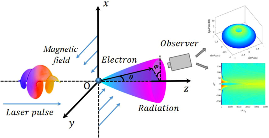
where $\stackrel{\rightharpoonup }{x}$ and $\stackrel{\rightharpoonup }{y}$ denote the unit vectors along the $+\widehat{x}$ and $+\widehat{y}$ directions, respectively. The first term on the right-hand side of Equation 1 describes a Hermite–Gaussian laser pulse with tightly focused circular polarization, $\delta =\pm 1$, as the laser pulses in this article are circularly polarized. We assume that the laser pulse propagates along $+\widehat{z}$. The peak amplitude of laser is $a_0=0.85\times {10}^{-9}\lambda \sqrt{I}$, and the laser intensity $I$ has been normalized by $m^2{c}^3{\omega }^2/e^2$, where $m$, $c$, $\omega$, and $e$ denote electron static mass, the light velocity in vacuum, the circular frequency of the incident laser, and a single electron’s charge, respectively. $a_L=a_0{b}_0\mathit{exp}\left(-{\eta }^2/L^2-{\rho }^2/b^2\right)/b$, where $\mathrm{\eta }=z-t$, $L$ is pulse width of the laser, and ${\rho }^2=x^2+y^2$, $b=b_0{\left(1+z^2/{Z_f}^2\right)}^{1/2}$ represents the radius of the light spot at a distance of z from the beam waist. To be more specific, $b_0$ is the minimum radius of laser’s beam waist, and $Z_f={b_0}^2/2$ is the Rayleigh distance. In terms of the phase $\phi$ in Equation 1, it can be described as $\mathrm{\phi }={\mathrm{\phi }}_0-{\phi }_G+{\phi }_r+\mathrm{\eta }$, where ${\mathrm{\phi }}_0$ stands for the laser pulse’s initial phase, ${\phi }_G=z/Z_f$ is the Gouy phase shift, ${\phi }_r={\rho }^2/\left(2R\left(z\right)\right)$ is the spherical wave phase shift, and $R\left(z\right)=z\left(1+{Z_f}^2/z^2\right)$ represents the radius of curvature of the isophase surface of the beam. To simplify the arithmetic, the inverse of $R$ is set as $R_f=\left({Z_f}^2+z^2\right)/z^2$. Then, it is easy to get ${\phi }_r={R_f\rho }^2/2$. The second term on the right-hand side of the Equation 1 describes an external magnetic field along the direction of $+\widehat{y}$. $B_0$ is the strength of the external magnetic field. All the units to $B_0$ below are in $kT$ [24]. The geometry of the combined field, the initial position of the electron, and the spatial distribution of radiation in the coordinate system are shown in Figure 1.

Figure 1

Figure 1. Schematic diagram for a tightly focused circularly polarized Hermite–Gaussian laser pulse and an external magnetic field. A relativistic electron is initially stationary at the origin of the coordinates. The length of the arrow indicating the direction of the magnetic field corresponds to the magnetic field strength at the corresponding location. We can obtain the spatial and frequency spectra of the radiated power from the observations, which are on the right side of the figure.

The equation of motion of an electron in an electromagnetic field can be obtained from the Lagrangian equation and the electron energy expression [16,24].

${\mathit{d}}_{\mathit{t}}\left(\stackrel{\rightharpoonup }{\mathit{p}}-\stackrel{\rightharpoonup }{\mathit{a}}\right)=-{\nabla }_{\mathit{a}}\left(\stackrel{\rightharpoonup }{\mathit{u}}·\stackrel{\rightharpoonup }{\mathit{a}}\right),(2)$

${\mathit{d}}_{\mathit{t}}\mathit{\gamma }=\stackrel{\rightharpoonup }{\mathit{u}}·{\mathit{\partial }}_{\mathit{t}}\stackrel{\rightharpoonup }{\mathit{a}},(3)$

where $\gamma ={\left(1-u^2\right)}^{-1/2}$ is the relativistic factor, $\stackrel{\rightharpoonup }{u}$ denotes the electron velocity that has been normalized by $c$, $\stackrel{\rightharpoonup }{p}=\gamma \stackrel{\rightharpoonup }{u}$ represents the electron momentum that has been normalized by $mc$, and $\stackrel{\rightharpoonup }{a}$ is the combined field vector potential expressed in Equation 1. ${\nabla }_a$ acts only on $\stackrel{\rightharpoonup }{a}$.

According to Equation 1, the components of $\stackrel{\rightharpoonup }{a}$ on $+\widehat{x}$, $+\widehat{y}$ can be expressed in the following forms, respectively, and we can get Equation 4 below,

$\left\{\begin{array}{l}{\mathit{a}}_{\mathit{x}}={\mathit{a}}_{\mathit{L}}\mathit{cos}\mathit{\phi }\\ {\mathit{a}}_{\mathit{y}}=\mathit{\delta }{\mathit{a}}_{\mathit{L}}\mathit{sin}\left(\mathit{\phi }\right)+{\mathit{B}}_{\mathbf{0}}\mathit{x}\end{array}\right..(4)$

Then, combining Equations 1–3, we can use Equation 5 to calculate the velocity and acceleration of the electron motion in the combined field in the components on the $+\widehat{x}$, $+\widehat{y}$ and $+\widehat{z}$ directions, respectively.

$\left\{\begin{array}{c}\mathit{\gamma }{\mathit{d}}_{\mathit{t}}{\mathit{u}}_{\mathit{x}}=\left(\mathbf{1}-{{\mathit{u}}_{\mathit{x}}}^{\mathbf{2}}\right){\mathit{\partial }}_{\mathit{t}}{\mathit{a}}_{\mathit{x}}+{\mathit{u}}_{\mathit{y}}\left({\mathit{\partial }}_{\mathit{y}}{\mathit{a}}_{\mathit{x}}-{\mathit{\partial }}_{\mathit{x}}{\mathit{a}}_{\mathit{y}}\right)+\dots \\ {\mathit{u}}_{\mathit{z}}\left({\mathit{\partial }}_{\mathit{z}}{\mathit{a}}_{\mathit{x}}-{\mathit{\partial }}_{\mathit{x}}{\mathit{a}}_{\mathit{z}}\right)-{\mathit{u}}_{\mathit{x}}{\mathit{u}}_{\mathit{y}}{\mathit{\partial }}_{\mathit{t}}{\mathit{a}}_{\mathit{y}}-{\mathit{u}}_{\mathit{x}}{\mathit{u}}_{\mathit{z}}{\mathit{\partial }}_{\mathit{t}}{\mathit{a}}_{\mathit{z}}\\ \mathit{\gamma }{\mathit{d}}_{\mathit{t}}{\mathit{u}}_{\mathit{y}}=\left(\mathbf{1}-{{\mathit{u}}_{\mathit{y}}}^{\mathbf{2}}\right){\mathit{\partial }}_{\mathit{t}}{\mathit{a}}_{\mathit{y}}+{\mathit{u}}_{\mathit{x}}\left({\mathit{\partial }}_{\mathit{x}}{\mathit{a}}_{\mathit{y}}-{\mathit{\partial }}_{\mathit{y}}{\mathit{a}}_{\mathit{x}}\right)+\dots ,\\ {\mathit{u}}_{\mathit{z}}\left({\mathit{\partial }}_{\mathit{z}}{\mathit{a}}_{\mathit{y}}-{\mathit{\partial }}_{\mathit{y}}{\mathit{a}}_{\mathit{z}}\right)-{\mathit{u}}_{\mathit{x}}{\mathit{u}}_{\mathit{y}}{\mathit{\partial }}_{\mathit{t}}{\mathit{a}}_{\mathit{x}}-{\mathit{u}}_{\mathit{y}}{\mathit{u}}_{\mathit{z}}{\mathit{\partial }}_{\mathit{t}}{\mathit{a}}_{\mathit{z}}\\ \mathit{\gamma }{\mathit{d}}_{\mathit{t}}{\mathit{u}}_{\mathit{z}}=\left(\mathbf{1}-{{\mathit{u}}_{\mathit{z}}}^{\mathbf{2}}\right){\mathit{\partial }}_{\mathit{t}}{\mathit{a}}_{\mathit{z}}+{\mathit{u}}_{\mathit{x}}\left({\mathit{\partial }}_{\mathit{x}}{\mathit{a}}_{\mathit{z}}-{\mathit{\partial }}_{\mathit{z}}{\mathit{a}}_{\mathit{x}}\right)+\dots \\ {\mathit{u}}_{\mathit{y}}\left({\mathit{\partial }}_{\mathit{y}}{\mathit{a}}_{\mathit{z}}-{\mathit{\partial }}_{\mathit{z}}{\mathit{a}}_{\mathit{y}}\right)-{\mathit{u}}_{\mathit{x}}{\mathit{u}}_{\mathit{z}}{\mathit{\partial }}_{\mathit{t}}{\mathit{a}}_{\mathit{x}}-{\mathit{u}}_{\mathit{y}}{\mathit{u}}_{\mathit{z}}{\mathit{\partial }}_{\mathit{t}}{\mathit{a}}_{\mathit{y}}\end{array}\right.(5)$

where $u_x$, $u_y$, and $u_z$ denote the electron velocity components in the $+\widehat{x}$, $+\widehat{y}$, $+\widehat{z}$ directions, respectively. Having determined the state of electron motion, the electromagnetic radiation in the combined field can be calculated. The power per unit angle, indicating the angular distribution of the instantaneous power, can be calculated using Equation 6:

$\frac{\mathit{d}\mathit{P}\left(\mathit{t}\right)}{\mathit{d}\mathbf{\Omega }}={\left[\frac{{\left|\stackrel{\rightharpoonup }{\mathit{n}}\times \left[\left(\stackrel{\rightharpoonup }{\mathit{n}}-\stackrel{\rightharpoonup }{\mathit{u}}\right)\times {\mathit{d}}_{\mathit{t}}\stackrel{\rightharpoonup }{\mathit{u}}\right]\right|}^{\mathbf{2}}}{{\left(\mathbf{1}-\stackrel{\rightharpoonup }{\mathit{n}}·\stackrel{\rightharpoonup }{\mathit{u}}\right)}^{\mathbf{6}}}\right]}_{{\mathit{t}}^{\prime }}(6)$

where the radiated power is normalized by ${\left({\omega }_{0}e\right)}^2/4\pi c$, $\stackrel{\rightharpoonup }{n}$ denotes the direction of radiation, $\stackrel{\rightharpoonup }{u}$ represents the electron velocity, $t^{\prime }$ denotes the moment when the radiation occurs, and $t$ is the moment at which the radiation is received by the observer.

The energy radiation per unit solid angle per unit frequency interval can be expressed as

$\frac{{\mathit{d}}^{\mathbf{2}}\mathit{I}}{\mathit{d}\mathit{\omega }\mathit{d}\mathbf{\Omega }}={\left|{\int }_{-\infty }^{\infty }\frac{\stackrel{\rightharpoonup }{\mathit{n}}\times \left[\left(\stackrel{\rightharpoonup }{\mathit{n}}-\stackrel{\rightharpoonup }{\mathit{u}}\right)\times {\mathit{d}}_{\mathit{t}}\stackrel{\rightharpoonup }{\mathit{u}}\right]}{{\left(\mathbf{1}-\stackrel{\rightharpoonup }{\mathit{n}}·\stackrel{\rightharpoonup }{\mathit{u}}\right)}^{\mathbf{2}}}{\mathit{e}}^{\mathit{i}\mathit{s}\left(\mathit{t}-\stackrel{\rightharpoonup }{\mathit{n}}·\stackrel{\rightharpoonup }{\mathit{r}}\right)}\mathit{d}\mathit{t}\right|}^{\mathbf{2}}(7)$

which is normalized by $e^2/4{\pi }^{2}c$. In Equation 7, $s={\omega }_f/{\omega }_0$, where ${\omega }_f$ is the frequency of the harmonic radiation.

3 Results

Consider a combined field consisting of a tightly focused circularly polarized Hermite–Gaussian laser pulse and an external magnetic field. In this paper, we study an underdense plasma consisting of electrons with a distance of $50{\lambda }_0$ or more between every two electrons. We can ignore the influence of the electric field that each electron is subjected to by the electrons around it, and they can be regarded as free electrons.

3.1 Comparison of electron trajectories at different peak amplitudes of a laser pulse

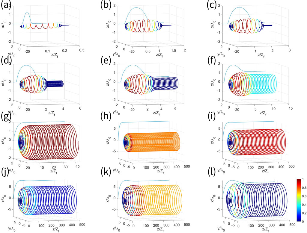
As shown in Figure 2, observing the electron motion trajectories, the electron is undergoing spiral motion in every plot, where the rotation axis is roughly along the $+\widehat{z}$ direction. We denote the $\widehat{z}$ direction as the transverse direction in the following. During this process, the transverse velocity $u_z$ and radial velocity $u_{\perp }$ of the electron are changing.

Figure 2

Figure 2. Trajectory driven by lasers with peak amplitude (a) ${\mathit{a}}_{\mathbf{0}}=\mathbf{1}$; (b) ${\mathit{a}}_{\mathbf{0}}=\mathbf{2.2}$; (c) ${\mathit{a}}_{\mathbf{0}}=\mathbf{2.4}$; (d) ${\mathit{a}}_{\mathbf{0}}=\mathbf{2.6}$; (e) ${\mathit{a}}_{\mathbf{0}}=\mathbf{2.7}$; (f) ${\mathit{a}}_{\mathbf{0}}=\mathbf{2.8}$; (g) ${\mathit{a}}_{\mathbf{0}}=\mathbf{3}$; (h) ${\mathit{a}}_{\mathbf{0}}=\mathbf{4}$; (i) ${\mathit{a}}_{\mathbf{0}}=\mathbf{6}$; (j) ${\mathit{a}}_{\mathbf{0}}=\mathbf{8}$; (k) ${\mathit{a}}_{\mathbf{0}}=\mathbf{10}$; and (l) ${\mathit{a}}_{\mathbf{0}}=\mathbf{20}$. The pulse width $\mathit{L}=\mathbf{5}{\mathit{\lambda }}_{\mathbf{0}}$, beam waist ${\mathit{b}}_{\mathbf{0}}=\mathbf{4}{\mathit{\lambda }}_{\mathbf{0}}$, and the strength of the external magnetic field ${\mathit{B}}_{\mathbf{0}}=\mathbf{0.5}\mathit{k}\mathit{T}$. Note the differences between the ranges of the coordinates of each plot. The solid curve in the $\mathit{x}\mathit{o}\mathit{y}$ plane represents the curve of the dependence of the electron energy on the z-coordinate value. The different colors on the trajectory curves indicate the corresponding position’s radiated power in the direction where the electron has the highest radiated power, which is normalized by the peak value of radiated power in each plot.

In order to better demonstrate the process of changes in electron energy as well as the radiated power during electron motion, we plot the electron trajectory, electron energy, and radiated power in every single plot, in which the curve of changes in electron energy is plotted in the $xoy$ plane, and the curve is plotted in different colors to vividly demonstrate the radiated power at the corresponding position in the direction of the greatest radiated power.

Note that in each plot, we have scaled down the height of the solid curve representing the electron energy by an equal amount to fit the range of the x- and y-coordinates on this plot. Therefore, this solid curve only reflects the change in electron energy with the z-coordinate in each plot, not the change in electron energy from plot to plot. In addition, in each plot, such radiated power is normalized by its peak in this plot. The ranges of the coordinates of each plot change to better show the trajectories under each group of parameters. In the first seven plots (a,b,c,d,e,f,g), the ranges of the x-coordinate and y-coordinate are both $\left(-2,2\right)$, while the range of the z-coordinate varies. In the last five plots (h,i,j,k,l), the ranges of the x- and y-coordinates are $\left(-8,8\right)$, and the range of the z-coordinates is $\left(0,500\right)$.

When $a_0<3$ (Figures 2a–f), the electron motion trajectory can be divided into two sections in the transverse direction in each trajectory plot. The first section’s radial distance from the rotation axis becomes smaller and larger with time, and the envelope takes on an olive shape. In this process, electron motion is mainly affected by the laser pulse. When the electron passes through the rising edge of the laser pulse, the electron energy increases, and the radius of the electron motion increases; when the electron passes through the falling edge of the laser pulse, the electron energy decreases, and the radius of the electron motion becomes smaller. The radial distance of the latter section remains relatively stable, and the envelope surface shows a cylindrical shape. This is because, at this time, the electron has been detached from the laser pulse and is only influenced by the applied magnetic field. That is to say, in the latter section, the electron makes a spiral motion with a constant radial distance, and the sparsity of the trajectory also remains constant. Then, the radial velocity $u_{\perp }$ and the transverse velocity $u_z$ undergo periodic changes, while the energy of the electron remains constant. The colors of the curves at different positions of the electron trajectory reflect the spatial variation of the radiated power. As time passes, the curve becomes redder, which means that the radiated power becomes larger. After the reddest point of the curve, the curve becomes bluer, meaning the radiated power becomes smaller. In the following parts of the paper, we describe the first and second sections of the spiral motion of the electron trajectory in terms of the olive and cylindrical forms, respectively, according to the above rules.

The variation of the electron trajectories with increasing peak amplitude, $a_0<3$ (Figures 2a–f), is discussed further specifically below. We analyze the olive state in the first section. In Figures 2a–f, the transverse displacements experienced by the electron during the period of the olive shape increase significantly with the increase of the peak amplitude $a_0$, and the transverse displacements range from approximately $0.25Z_f$ (Figure 2a) to approximately $7Z_f$ (Figure 2f). As the peak amplitude $a_0$ increases, the trajectory at the corresponding position becomes thinner and thinner, the transverse displacement of the electrons moving to the maximum radial distance increases, and the maximum radial distance increases by a small amount. This is because, as $a_0$ increases, the electron is accelerated more strongly by the rising edge of the laser, and the maximum radial distance increases as a result. This further leads to an enhancement of the Lorentz force generated by the radial velocity $u_{\perp }$ on the electron, leading to an increase in the transverse velocity $u_z$ of the electron. Therefore, the trajectories at the corresponding positions on the different plots become thinner and thinner as $a_0$ increases, and the transverse displacement at which the maximum radial distance is reached increases as a result.

In the cylindrical shape of the latter section, the electron is no longer subjected to the laser pulse but moves in a spiral motion at a certain energy under the action of the magnetic field alone. In Figures 2a–f, the radial radius of the trajectories in this section increases significantly with the increase of the peak amplitude $a_0$, and the radial radius goes from close to $0$ (Figure 2a), to $0.049{\lambda }_0$ (Figure 2c), to $0.639{\lambda }_0$ (Figure 2e), and to $1.057{\lambda }_0$ (Figure 2f). The radiative power in this position becomes smaller and the electron helical trajectory becomes thinner and thinner. Interestingly, more and more ends of the olive shape are replaced by the cylindrical shape at the connection between the two shapes. Although the radial distances of both the olive and cylindrical shapes are increasing, the growth rate of the latter is much larger than that of the former, so it appears that the cylindrical shapes gradually annex the olive form. This is because, as stated above, an increase in $a_0$ leads to an increase in radial velocity $u_{\perp }$, transverse velocity $u_z$, and these lead to an increase in the Lorentz force. The increase in $a_0$ causes the external magnetic field to have a strong effect on the electron trajectory. Even the process where the electron moves in a smaller radial distance in response to the falling edge of the laser pulse is no longer complete. The second half of this process is replaced by a spiral motion with constant radial distance caused by the strong Lorentz force.

When ${3<a}_0<10$ (Figures 2g–k), the electron motion trajectory observed from the viewpoint shown in Figure 2 takes on the shape of a closed left side and an open right side. The electron starts to move from the action of the laser pulse, and the radial distance away from the rotation axis first becomes larger and larger with time, after which the electron moves in a spiral motion, with a radial distance that tends to be constant, and the energy of the electron also remains constant. At this time, as the peak amplitude $a_0$ increases, the number of electrons rotating through the circle decreases when the electron in the acceleration process reaches the maximum radial distance. The radial distance also increases with $a_0$ as it eventually remains stable. This is because under the action of the external magnetic field, the Lorentz force, which becomes stronger and stronger as the peak amplitude $a_0$ increases, makes the process of decreasing radial distance brought about by the falling edge of the laser pulse to be completely absorbed by the helical motion afterward. The transverse velocity $u_z$, which increases with $a_0$, allows the electron to reach the peak position of the laser pulse more quickly, so the rotational period spent becomes shorter. The larger peak amplitude causes stronger acceleration, and the final radial distance increases as a result.

Interestingly, in this phase, the color change of the trajectory reflects the brand-new pattern of change of the radiant power. On the one hand, the general trend shows that the radiant power first increases before decreasing to a steady stage. It is easy to understand. We know that electrons experience the sequential action of the rising and falling edges of the pulse. During the rising edge portion, the gradient becomes larger first. Then, somewhere before the pulse peaks, the gradient begins to decrease. Thus, a change in the gradient results in a change in electron acceleration. This process typically involves an initial increase followed by a decrease, which in turn affects the radiated power in a similar manner. On the other hand, by observing the localized variations of the radiated power, it can be noticed that there are localized oscillations in the phase of the overall upward trend of the power discussed above. This is due to the competition between the applied magnetic field and the electric field under the laser pulse. As the peak amplitude increases, such a competitive relationship becomes more pronounced. This is because an increase in the peak amplitude causes an increase in the gradient, and the electric field becomes stronger. Based on what has been analyzed above, it can be seen that a greater radial distance in this case results in a stronger magnetic field. As a result, there is a larger tug of war between the stronger electric field and the stronger magnetic field, so the amplitude of the oscillations becomes larger, thus leading to a more pronounced change in the color of the curve in the plots.

When ${10<a}_0\le 20$, because there is no obvious change in the electron motion trajectory in this process with the increase of the peak amplitude $a_0$, only the most obvious feature $a_0=20$ (Figure 2l) is selected for analysis. When ${10<a}_0\le 20$, as time progresses, the radial distance from the rotation axis first increases, then decreases, and eventually stabilizes. In addition, similar trajectory shapes occur when $a_0$ is small. There are cases when the radial distance is small in $a_0=1$ at approximately $0.25{\lambda }_0$ (Figure 2a), and in $a_0=2.8$, at about $7{\lambda }_0$ (Figure 2f). In comparison, at $a_0=20$, the radial distance is very large when the trend of decreasing radial distance ends and remains stable at approximately $200{\lambda }_0$. The phenomenon of increase in radial distance followed by a decrease is increasingly significant as the peak amplitude increases. This is because when $a_0>10$, due to the further increase of the peak amplitude $a_0$, the falling edge of the laser pulse becomes steeper, then the effect of the falling edge is more significant compared with the effect of the applied magnetic field. Then, the effect of the falling edge gradually regains the dominant position. In this situation, the trajectory of the electron again appears to change in a similar way as before, with the radial distance becoming larger and then smaller.

We know that the rising edge of the laser pulse increases the electron energy, and the falling edge decreases the electron energy. By applying a magnetic field, we find that the parameter $a_0=10$ (Figure 2k) gives the electron a higher energy. At this point, the electron does not undergo the process of decreasing radial distance caused by the falling edge. Parameter $a_0=10$ gives the electron the largest final radial radius of all peak amplitude parameters that satisfy this condition.

3.2 Comparison of spatial radiation at different peak amplitudes of laser pulse

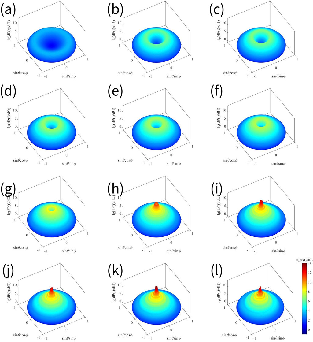
In the full space, for each unit of solid angle, we find the radiated power when it reaches its maximum value throughout the process, and then we define this power as this unit of solid angle’s maximum radiated power in full time, which is expressed by $dP\left(t\right)/d\mathrm{\Omega }$. We abbreviate it as the radiated power per unit of solid angle. The maximum of the $dP\left(t\right)/d\mathrm{\Omega }$ of all unit solid angles in the whole space is taken as the maximum value $\mathit{max}\left[dP\left(t\right)/d\mathrm{\Omega }\right]$. In the following content, we will call it the maximum radiated power per unit solid angle. The direction in which this solid angle is located is defined as the direction of maximum radiated power per unit solid angle, denoted by $\left({\theta }_m,{\phi }_m\right)$. Then, the space radiation brought about by electron scattering is plotted in a column coordinate system. Specifically, the direction of the unit solid angle in space is represented on a plane, and the vertical height of the three-dimensional figure is used to represent the radiated power per unit of solid angle $dP\left(t\right)/d\mathrm{\Omega }$, as shown in Figure 3. On the surface of a sphere of radius 1, the coordinates of a point P are $\left(x_p,y_p,z_p\right)$, which is at a distance of $1$ from the coordinate origin $O$, and $\stackrel{\rightharpoonup }{OP}$ denotes the unit vector in the direction of radiation. $x_p=\sin {\theta }_P\cos {\phi }_P$, $y_p=\sin {\theta }_P\sin {\phi }_P$, denoting the horizontal and vertical coordinates of point P in the plane, respectively. The spatial radiation at different peak amplitudes of the laser pulse is shown in Figure 3, where the logarithm of 10 is taken for $dP\left(t\right)/d\mathrm{\Omega }$. The value of the radiated power per unit of solid angle can not only be reflected by the height on the vertical axis; it can also be reflected by the color temperature, where a higher color temperature means that $dP\left(t\right)/d\mathrm{\Omega }$ is larger.

Figure 3

Figure 3. Distribution of maximum radiated power per unit solid angle $\mathit{d}\mathit{P}\left(\mathit{t}\right)/\mathit{d}\mathit{\Omega }$ for electron scattering in lasers with peak amplitude (a) ${\mathit{a}}_{\mathbf{0}}=\mathbf{1}$; (b) ${\mathit{a}}_{\mathbf{0}}=\mathbf{2.2}$; (c) ${\mathit{a}}_{\mathbf{0}}=\mathbf{2.4}$; (d) ${\mathit{a}}_{\mathbf{0}}=\mathbf{2.6}$; (e) ${\mathit{a}}_{\mathbf{0}}=\mathbf{2.7}$; (f) ${\mathit{a}}_{\mathbf{0}}=\mathbf{2.8}$; (g) ${\mathit{a}}_{\mathbf{0}}=\mathbf{3}$; (h) ${\mathit{a}}_{\mathbf{0}}=\mathbf{4}$; (i) ${\mathit{a}}_{\mathbf{0}}=\mathbf{6}$; (j) ${\mathit{a}}_{\mathbf{0}}=\mathbf{8}$; (k) ${\mathit{a}}_{\mathbf{0}}=\mathbf{10}$; and (l) ${\mathit{a}}_{\mathbf{0}}=\mathbf{20}$. The pulse width $\mathit{L}=\mathbf{5}{\mathit{\lambda }}_{\mathbf{0}}$, beam waist ${\mathit{b}}_{\mathbf{0}}=\mathbf{4}{\mathit{\lambda }}_{\mathbf{0}}$, and the strength of the external magnetic field ${\mathit{B}}_{\mathbf{0}}=\mathbf{0.5}\mathit{k}\mathit{T}$.

When $a_0<3$ (Figures 3a–f), the shape of the spatial radiation distribution of electron Thomson scattering approximates the shape of a volcano with a large opening in the center. As the polar angle $\theta$ gradually changes from $\pi /2$ to $0$, the radiated power per unit solid angle $dP\left(t\right)/d\mathrm{\Omega }$ first increases at a slower rate as the polar angle $\theta$ gets smaller until it reaches the maximum value $\mathit{max}\left[dP\left(t\right)/d\mathrm{\Omega }\right]$. Subsequently, as the polar angle $\theta$ continues to decrease from ${\theta =\theta }_m$, the radiated power $dP\left(t\right)/d\mathrm{\Omega }$ decreases to zero at a very rapid rate.

The variation of the maximum radiated power per unit solid angle with the increase of the peak amplitude $a_0$ in the case of $a_0<3$ (Figures 3a–f) is discussed further below. As the peak amplitude $a_0$ of the laser pulse increases, the opening at the upper end of the shape becomes significantly smaller, indicating that the polar angle ${\theta }_m$ in the direction of the maximum radiated power becomes substantially smaller. In addition, the maximum radiated power in full space and full time also increases significantly with the increase of the peak amplitude. In particular, for $a_0=1$ (Figure 3a), the shape of the graph is more like a blood cell, as evidenced by its larger ${\theta }_m$ and smaller value of $\mathit{max}\left[dP\left(t\right)/d\mathrm{\Omega }\right]$.

When ${3\le a}_0<10$ (Figures 3g–k), every plot takes on an inverted eddy shape that is wound around itself from the outer ring to the center, and its height gradually increases. Figuratively speaking, the swirl here is narrow at the top and wide at the bottom, upside down from the eddy of water and wind in nature. In general, on the basis of the original volcanic shape of the outer rim, high-power radiation with a steeply increasing height and a radius concentrated around $\sin {\theta }_m$ appears in the inner rim. Specifically, as the polar angle $\theta$ gradually changes from $\pi /2$ to $0$, the texture of the swirl gradually turns into a protrusion of a tangible inverted eddy. As for the change in power, as the polar angle $\theta$ becomes smaller, the radiated power per unit of solid angle $dP\left(t\right)/d\mathrm{\Omega }$ first increases slowly. Then, this increase to the maximum value $\mathit{max}\left[dP\left(t\right)/d\mathrm{\Omega }\right]$ is particularly noticeable. After that, it decreases sharply to zero. In addition, the spatial distribution of the radiated power appears to be significantly asymmetric due to the appearance of an inverted eddy pattern.

The variation of the maximum radiated power per unit solid angle with increasing peak amplitude $a_0$ for the case ${3\le a}_0<10$ (Figures 3g–k) is discussed below. As $a_0$ increases, the maximum radiated power angle ${\theta }_m$ slowly becomes smaller, and the collimation of radiation has a weak enhancement. The maximum radiated power is affected by the peak amplitude and shows a rapid increase.

It is worth noting that the maximum radiated power per unit solid angle, $\mathit{max}\left[dP\left(t\right)/d\mathrm{\Omega }\right]$, does not continuously increase with the peak amplitude $a_0$. The $\mathit{max}\left[dP\left(t\right)/d\mathrm{\Omega }\right]$ in $a_0=10$ (Figure 3k) is significantly larger than that in $a_0=20$ (Figure 3l).

This is seen below in conjunction with the electron trajectory diagram in Figure 2. The direction of radiation coincides with the direction of electron velocity, which is the tangent direction of the electron trajectory [17]. In Figure 3, as the peak amplitude becomes larger, the electron acquires a larger transverse velocity $u_z$, which in turn causes the component of the radiation direction in the $+\widehat{z}$ direction to appear to be dramatically increased. While the electron is subject to the successive effects of periodic acceleration and deceleration of the magnetic field in the radial direction, the velocity direction, which is the component of the radiation direction in the $+\widehat{x}$ and $+\widehat{y}$ directions, varies by a small amount. Therefore, the radiation direction generally shows a tendency of constant inclination to the $+\widehat{z}$ direction, which is consistent with the phenomenon that the radiation collimation becomes better with the increase of the peak amplitude, as presented in Figure 3.

3.3 Comparison of spatial spectra of laser pulses at different peak amplitudes

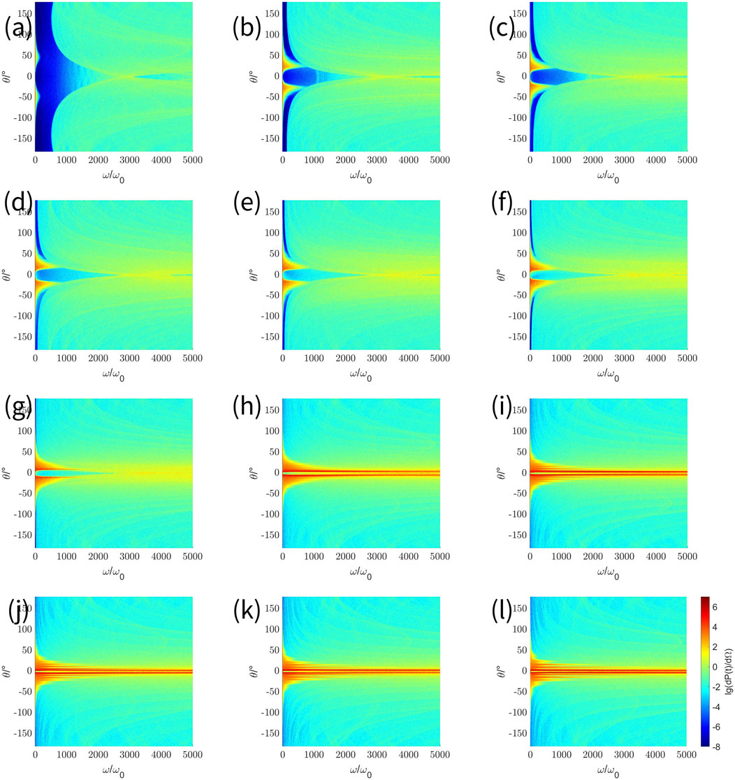
The power spectrum at $\theta$ in the angular range of $\left(-180°,180°\right)$ is presented in Figure 4, using $\theta$ and $\omega /{\omega }_0$ as horizontal and vertical coordinates, respectively, where the range of values of $\omega /{\omega }_0$ is uniformly $\left(0,5000\right)$. The logarithm of 10 is taken for the radiated power in order to better present the process of change between each plot. The color temperature reflects the value of the radiant power, where a higher color temperature indicates a higher radiant power. With this section, we analyze the distribution of the radiated power spectrum over different polar angles.

Figure 4

Figure 4. Spectra of radiated power in the direction of each polar angle $\mathit{\theta }$ at the azimuth of maximum radiation, where the peak amplitude of the laser pulse in each graph is (a) ${\mathit{a}}_{\mathbf{0}}=\mathbf{1}$; (b) ${\mathit{a}}_{\mathbf{0}}=\mathbf{2.2}$; (c) ${\mathit{a}}_{\mathbf{0}}=\mathbf{2.4}$; (d) ${\mathit{a}}_{\mathbf{0}}=\mathbf{2.6}$; (e) ${\mathit{a}}_{\mathbf{0}}=\mathbf{2.7}$; (f) ${\mathit{a}}_{\mathbf{0}}=\mathbf{2.8}$; (g) ${\mathit{a}}_{\mathbf{0}}=\mathbf{3}$; (h) ${\mathit{a}}_{\mathbf{0}}=\mathbf{4}$; (i) ${\mathit{a}}_{\mathbf{0}}=\mathbf{6}$; (j) ${\mathit{a}}_{\mathbf{0}}=\mathbf{8}$; (k) ${\mathit{a}}_{\mathbf{0}}=\mathbf{10}$; and (l) ${\mathit{a}}_{\mathbf{0}}=\mathbf{20}$. The pulse width $\mathit{L}=\mathbf{5}{\mathit{\lambda }}_{\mathbf{0}}$, beam waist ${\mathit{b}}_{\mathbf{0}}=\mathbf{4}{\mathit{\lambda }}_{\mathbf{0}}$, and the strength of the external magnetic field ${\mathit{B}}_{\mathbf{0}}=\mathbf{0.5}\mathit{k}\mathit{T}$.

When $a_0<3$ (Figures 4a–f), the polar angle $\theta$ can be divided into two ranges, $\left(0°,180°\right)$ and $\left(-180°,0°\right)$, which correspond to the figure’s upper and lower parts bounded by $\theta =0°$, respectively. To omit repetitive descriptions, only the range of $\left(0°,180°\right)$ is described below because the two parts are roughly symmetrical on the axis of $\theta =0°$. We know that when $\theta$ takes a particular value, it enables the power spectrum to have the maximum cutoff frequency with the maximum power and the radiated power to reach the maximum. It is the angle that we mentioned in Section 3.2, which is the polar angle ${\theta }_m$ where radiated power becomes maximum. We investigate the power spectrum in the direction of ${\theta }_m$. Starting from the fundamental frequency, as the number of harmonics increases, the power increases rapidly. After peaking, it falls back to zero. In each plot, the cutoff frequency of the power spectrum in each $\theta$ direction becomes first larger and then smaller as $\theta$ decreases. Whereas ${\theta }_m$ lies in the angular range of $∆\theta$, where the harmonics in the power spectrum can be observed more clearly. For the part outside the angular range of $∆\theta$, there are almost no high harmonics, and the cutoff frequency is very small. As the number of harmonics increases, the power decreases to 0 very quickly, but a very small amount of power occurs at higher frequencies.

When ${3\le a}_0<10$ (Figures 4g–k), there are very pronounced high harmonics in the direction of ${\theta }_m$. Interestingly, in this case, the cutoff frequency no longer shows a gradual increase as the polar angle gets closer to ${\theta }_m$ in (Figures 4a–l). In fact, in the vicinity of ${\theta }_m$, the positions of the distributions of a series of cutoff frequencies at different $\theta$ directions appear as a clearly spaced sequence of peaks and valleys. That is to say, the polar angle directions with larger cutoff frequencies occur at intervals. The peaks correspond to the direction of the polar angle with the larger cutoff frequency, while the valleys between the two peaks correspond to the direction of the polar angle with a smaller cutoff frequency. The phenomenon is consistent with the morphology of the inverted eddy described in Section 3.2, in which there is a certain gap between each of the polar angles with large radiated power, observed from the same $\phi$ position.

The spectrograms at different peak amplitudes are compared below. As the peak amplitude increases, the cutoff frequency increases. Specifically, in the case of $a_0<3$, the radiated power at ${\theta }_m$ has already shown a large attenuation when $\omega /{\omega }_0=1000$, while in the case of $a_0>3$, there is still a large radiated power at the position of $\omega /{\omega }_0=5000$. In addition, ${\theta }_m$ decreases with increasing peak amplitude, which suggests that an increase in peak amplitude can greatly improve the collimation of radiation. When the peak amplitude continues to increase from $a_0=3$, ${\theta }_m$ decreases at an extremely slow rate and finally tends to a stable value.

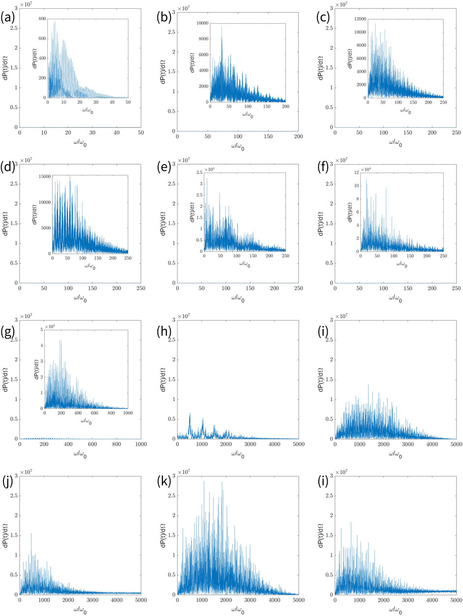
We are more interested in the spectrum in the direction of the polar angle ${\theta }_m$, where radiated power becomes maximum, rather than the direction of other ordinary polar angle $\theta$ where the power is less and the number of harmonics is lower. In Figure 4, we slice the location of ${\theta }_m$ as shown in Figure 5 below. In the following, we further investigate the spectrum specifically in the direction of ${\theta }_m$.

Figure 5

Figure 5. Spectrogram of the maximum radiated power in the direction of $\left({\mathit{\theta }}_{\mathit{m}},{\mathit{\phi }}_{\mathit{m}}\right)$, where the peak amplitude of the laser pulse in each graph is (a) ${\mathit{a}}_{\mathbf{0}}=\mathbf{1}$; (b) ${\mathit{a}}_{\mathbf{0}}=\mathbf{2.2}$; (c) ${\mathit{a}}_{\mathbf{0}}=\mathbf{2.4}$; (d) ${\mathit{a}}_{\mathbf{0}}=\mathbf{2.6}$; (e) ${\mathit{a}}_{\mathbf{0}}=\mathbf{2.7}$; (f) ${\mathit{a}}_{\mathbf{0}}=\mathbf{2.8}$; (g) ${\mathit{a}}_{\mathbf{0}}=\mathbf{3}$; (h) ${\mathit{a}}_{\mathbf{0}}=\mathbf{4}$; (i) ${\mathit{a}}_{\mathbf{0}}=\mathbf{6}$; (j) ${\mathit{a}}_{\mathbf{0}}=\mathbf{8}$; (k) ${\mathit{a}}_{\mathbf{0}}=\mathbf{10}$; and (l) ${\mathit{a}}_{\mathbf{0}}=\mathbf{20}$. The pulse width $\mathit{L}=\mathbf{5}{\mathit{\lambda }}_{\mathbf{0}}$, beam waist ${\mathit{b}}_{\mathbf{0}}=\mathbf{4}{\mathit{\lambda }}_{\mathbf{0}}$, and the strength of the external magnetic field ${\mathit{B}}_{\mathbf{0}}=\mathbf{0.5}\mathit{k}\mathit{T}$. Note the difference in the range of horizontal and vertical coordinates for each of the smaller plots appended in (a–g) and the difference in the range of horizontal coordinates for the larger plots in (a–g). The vertical coordinate is normalized by ${\left({\mathit{\omega }}_{\mathbf{0}}\mathit{e}\right)}^{\mathbf{2}}/\mathbf{4}\mathit{\pi }\mathit{c}$.

When $a_0<3$ (Figures 5a–f), the radiated power per unit solid angle increases rapidly as the peak amplitude increases. Taking the maximum power $\mathit{max}\left[dP\left(t\right)/d\mathrm{\Omega }\right]$ in each plot as an example: the maximum power in $a_0=1$ (Figure 5a) is approximately 780, and then it gradually becomes approximately 15,000 ($a_0=2.6$, Figure 5d) and increases again to hundreds of thousands ($a_0=2.7$, Figure 5e). In addition, the number of harmonics keeps increasing. For ease of description, in the case of different peak amplitudes, we name the number of harmonics at which the power decays to one-tenth of the maximum power value as ${\left(\omega /{\omega }_0\right)}_d$. As the peak amplitude increases, ${\left(\omega /{\omega }_0\right)}_d$ varies from the initial ${\left(\omega /{\omega }_0\right)}_d=28$ (Figure 5a), to ${\left(\omega /{\omega }_0\right)}_d=158$ in $a_0=2.2$ (Figure 5b), and, to ${\left(\omega /{\omega }_0\right)}_d=689$ in $a_0=3$ (Figure 5g). It can be seen that only a small increase in peak amplitude from $a_0=1$ to $a_0=3$ causes a significant increase in harmonic number.

When ${3\le a}_0<10$ (Figures 5g–k), the maximum radiated power per unit solid angle $\mathit{max}\left[dP\left(t\right)/d\mathrm{\Omega }\right]$ continues to increase as the peak amplitude increases, but the increase is small, and the order of magnitude does not change. At the highest point, for example, the orders of magnitude all remain at ${10}^7$. On the other hand, the number of harmonics continues to increase, from ${\left(\omega /{\omega }_0\right)}_d=3194$ when $a_0=4$ (Figure 5h), to ${\left(\omega /{\omega }_0\right)}_d=3804$ when $a_0=6$ (Figure 5i), to ${\left(\omega /{\omega }_0\right)}_d=4196$ when $a_0=10$ (Figure 5k). However, when $a_0=20$ (Figure 5l), the maximum radiated power per unit solid angle $\mathit{max}\left[dP\left(t\right)/d\mathrm{\Omega }\right]$ is smaller than that in $a_0=10$, and ${\left(\omega /{\omega }_0\right)}_d$ is also smaller at 3,584.

It is worth noting that this is not a discrete spectrum but a supercontinuous spectrum. This is because a portion of the radiation in the vicinity of the direction of maximum radiation $\left({\theta }_m,{\phi }_m\right)$ can also be observed in the direction of $\left({\theta }_m,{\phi }_m\right)$. Although the radiated power observed in the direction of $\left({\theta }_m,{\phi }_m\right)$ is dominated by the radiated power that is generated exactly in the direction of $\left({\theta }_m,{\phi }_m\right)$, we actually observe the superposition of the spectra in more than one direction. This is why Figure 5 presents a continuous spectral distribution.

3.4 Dependence of maximum radiated power per unit solid angle on magnetic field strength

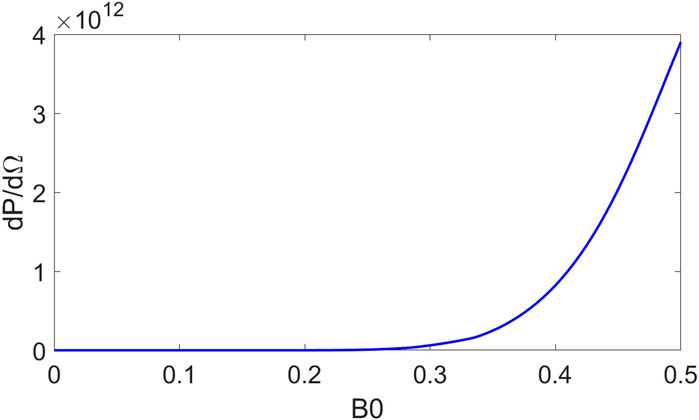
With specific parameters ($a_0=5$, $L=5{\lambda }_0$, $b_0=4{\lambda }_0$), we plotted the variation of maximum radiated power per unit solid angle $\mathit{max}\left[dP\left(t\right)/d\mathrm{\Omega }\right]$ with the magnetic field strength ${\mathit{B}}_{\mathbf{0}}$. The results are shown in Figure 6.

Figure 6

Figure 6. A line graph showing the dependence of maximum radiated power per unit solid angle $\mathit{max}\left[\mathit{d}\mathit{P}\left(\mathit{t}\right)/\mathit{d}\mathit{\Omega }\right]$ on the magnetic field strength ${\mathit{B}}_{\mathbf{0}}$. The horizontal coordinate magnetic field strength ${\mathit{B}}_{\mathbf{0}}$ is in the range $\left[\mathbf{0},\mathbf{0.5}\right]$. The vertical coordinate maximum radiated power per unit solid angle $\mathit{max}\left[\mathit{d}\mathit{P}\left(\mathit{t}\right)/\mathit{d}\mathit{\Omega }\right]$ is in the range $\left[\mathbf{0},\mathbf{0.5}\right]$. The laser pulse peak amplitude ${\mathit{a}}_{\mathbf{0}}=\mathbf{5}$, pulse width $\mathit{L}=\mathbf{5}{\mathit{\lambda }}_{\mathbf{0}}$, beam waist ${\mathit{b}}_{\mathbf{0}}=\mathbf{4}{\mathit{\lambda }}_{\mathbf{0}}$, and the strength of the external magnetic field ${\mathit{B}}_{\mathbf{0}}=\mathbf{0.5}\mathit{k}\mathit{T}$. Note that the maximum radiated power per unit solid angle is normalized by ${\left({\mathit{\omega }}_{\mathbf{0}}\mathit{e}\right)}^{\mathbf{2}}/\mathbf{4}\mathit{\pi }\mathit{c}$.

The graph above describes the dependence of maximum radiated power per unit solid angle $\mathit{max}\left[dP\left(t\right)/d\mathrm{\Omega }\right]$ on the magnetic field strength $B_0$ when $a_0=5$, $L=5{\lambda }_0$, $b_0=4{\lambda }_0$. The horizontal coordinate magnetic field strength $B_0$ is in the range of $\left[0,0.5\right]$. The vertical coordinate maximum radiated power per unit solid angle $\mathit{max}\left[dP\left(t\right)/d\mathrm{\Omega }\right]$ is in the range of $\left[0,0.5\right]$. Note that the maximum radiated power per unit solid angle is normalized by ${\left({\omega }_{0}e\right)}^2/4\pi c$.

As can be seen from the above figure, with the above parameters, as the magnetic field strength increases, the maximum radiated power per unit solid angle also increases significantly. That is, the addition of the magnetic field greatly enhances the $\mathit{max}\left[dP\left(t\right)/d\mathrm{\Omega }\right]$. This is consistent with our previous analysis. The radial distance of electron motion increases when the electron is accelerated by the rising edge of the laser. The greater magnetic field strength at the greater radial distance enhances the Lorentz force on the electron generated by the radial velocity $u_{\perp }$, resulting in an increase in the electron’s transverse velocity $u_z$. The increase in $u_z$ results in the electron being subjected to an even greater radial Lorentz force, and so the radial distance is further increased. The addition of the magnetic field causes a large increase in the total velocity u of the electrons and a corresponding increase in the maximum velocity that the electrons can achieve. The larger the magnetic field strength $B_0$ is, the more significant the enhancement of electron velocity is.

We analyze the following according to Equation 6. The rise of the total velocity $u$ makes the denominator ${\left(1-\stackrel{\rightharpoonup }{n}·\stackrel{\rightharpoonup }{u}\right)}^6$ at the right side of Equation 6 get closer and closer to 0, and then the whole equation increases. That is, the increase in the maximum electron velocity increases $\mathit{max}\left[dP\left(t\right)/d\mathrm{\Omega }\right]$.

Overall, the addition of the magnetic field greatly enhances the $\mathit{max}\left[dP\left(t\right)/d\mathrm{\Omega }\right]$, and as the magnetic field strength $B_0$ increases, the maximum radiated power per unit solid angle $\mathit{max}\left[dP\left(t\right)/d\mathrm{\Omega }\right]$ increases.

3.5 Dependence of the polar angle where radiated power becomes maximum and the maximum radiated power per unit solid angle on the peak amplitude of the laser pulse

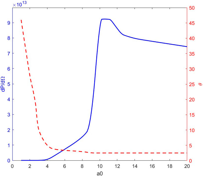
A two-coordinate plot was drawn based on the polar angle ${\theta }_m,$ where the radiated power becomes maximum, and the maximum radiated power per unit solid angle can be described by $\mathit{max}\left[dP\left(t\right)/d\mathrm{\Omega }\right]$ at different peak amplitudes $a_0$. This is shown in Figure 7.

Figure 7

Figure 7. A biaxial plot showing the dependence of the polar angle ${\mathit{\theta }}_{\mathit{m}}$, where the radiated power becomes maximum (dashed curve), and the maximum radiated power per unit solid angle can be described by $\mathit{max}\left[\mathit{d}\mathit{P}\left(\mathit{t}\right)/\mathit{d}\mathit{\Omega }\right]$ (solid curve) on the laser pulse peak amplitude ${\mathit{a}}_{\mathbf{0}}$, respectively. The horizontal coordinate peak amplitude ${\mathit{a}}_{\mathbf{0}}$ is in the range $\left[\mathbf{1},\mathbf{20}\right]$. The pulse width $\mathit{L}=\mathbf{5}{\mathit{\lambda }}_{\mathbf{0}}$, beam waist ${\mathit{b}}_{\mathbf{0}}=\mathbf{4}{\mathit{\lambda }}_{\mathbf{0}}$, and the strength of the external magnetic field ${\mathit{B}}_{\mathbf{0}}=\mathbf{0.5}\mathit{k}\mathit{T}$. Note that the maximum radiated power per unit solid angle is normalized by ${\left({\mathit{\omega }}_{\mathbf{0}}\mathit{e}\right)}^{\mathbf{2}}/\mathbf{4}\mathit{\pi }\mathit{c}$.

The graph above describes the dependence of the polar angle ${\theta }_m$, where the radiated power becomes maximum, and the maximum radiated power per unit solid angle can be described by $\mathit{max}\left[dP\left(t\right)/d\mathrm{\Omega }\right]$ on the laser pulse peak amplitude $a_0$, respectively. The horizontal coordinate peak amplitude $a_0$ is in the range $\left[1,20\right]$. The solid curve indicates the variation of $\mathit{max}\left[dP\left(t\right)/d\mathrm{\Omega }\right]$ and corresponds to the left vertical axis. The dashed curve shows the variation of ${\theta }_m$ and corresponds to the right vertical axis. Note that $\mathit{max}\left[dP\left(t\right)/d\mathrm{\Omega }\right]$ is normalized by ${\left({\omega }_{0}e\right)}^2/4\pi c$.

We first analyze the dependence of the polar angle ${\theta }_m$, where the radiated power becomes maximum on the laser pulse peak amplitude $a_0$ (dashed curve).

Overall, ${\theta }_m$ decreases with increasing peak amplitude. Specifically, the rate at which ${\theta }_m$ decreases is significantly different for different ranges of $a_0$. When $a_0<3$, ${\theta }_m$ decreases dramatically with increasing peak amplitude. From ${\theta }_m=46°\left(a_0=1\right)$, to ${\theta }_m=25°\left(a_0=2.2\right)$, to ${\theta }_m=14°\left(a_0=2.8\right)$, the polar angle ${\theta }_m$ decreases by nearly a quarter. That is to say, the collimation of the radiation becomes significantly better at this stage. When ${3<a}_0<10$, ${\theta }_m$ decreases more slowly as the peak amplitude increases. After that, when $a_0>10$, ${\theta }_m$ decreases very little and hardly changes, and finally ${\theta }_m$ is about 2.5°. In terms of ${\theta }_m$, the peak amplitude $a_0$ should be as large as possible in order to obtain the best collimation. However, the variation of collimation is extremely slight after $a_0>10$. Considering the cost and difficulty of realization in engineering, $a_0=10$ can be approximated as the best point of collimation in the range of $\left[1,20\right]$.

We continue to analyze the dependence of the maximum radiated power per unit solid angle $\mathit{max}\left[dP\left(t\right)/d\mathrm{\Omega }\right]$ on the laser pulse peak amplitude $a_0$ (solid curve).

From the general trend, $\mathit{max}\left[dP\left(t\right)/d\mathrm{\Omega }\right]$ increases and then decreases with $a_0=10$ as the boundary. When $a_0<3$, $\mathit{max}\left[dP\left(t\right)/d\mathrm{\Omega }\right]$ changes slightly. When ${3<a}_0<10$, $\mathit{max}\left[dP\left(t\right)/d\mathrm{\Omega }\right]$ appears to rise sharply as the peak amplitude increases. It is noteworthy that when $a_0>10$, $\mathit{max}\left[dP\left(t\right)/d\mathrm{\Omega }\right]$ decreases slowly, although the peak amplitude further increases. Therefore, the peak of $\mathit{max}\left[dP\left(t\right)/d\mathrm{\Omega }\right]$ is reached at $a_0=10$.

In summary, when $a_0=10$, we can obtain not only the best collimation but also the strongest radiated power. Therefore, when the pulse width $L=5{\lambda }_0$, and the beam waist $b_0=4{\lambda }_0$, the strength of the external magnetic field $B_0=0.5$, and the optimal parameter for the peak amplitude is $a_0=10$.

4 Discussion

First, we discuss Figure 2. When $a_0<3$ (Figures 2a–f), the envelope of the electron trajectory presents a combination of olive and cylindrical shapes. When ${3<a}_0<10$ (Figures 2g–k), the envelope of the electron trajectory presents a shape with a closed left side and an open right side. When ${10<a}_0\le 20$, the radial distance of the motion trajectory becomes larger and then smaller. Among the above parameters, we find that the parameter $a_0=10$ (Figure 2k) enables the electron to obtain higher energy. At this point the electron both happens to not undergo the process of decreasing radial distance caused by the falling edge. $a_0=10$ is the parameter that gives the electron the largest final radial radius of all the peak amplitude parameters that satisfy this condition. A discussion of Figure 3 follows. When $a_0<3$ (Figures 3a–f), the shape of the spatial radiation distribution approximates the shape of a volcano with a large opening in the middle. When ${3<a}_0<10$ (Figures 3g–k), every plot takes on an inverted eddy shape that is wound around itself from the outer ring to the center, and its height gradually increases. As the peak amplitude increases, the polar angle in the direction of the maximum radiated power ${\theta }_m$ decreases rapidly before gradually increasing.

Where $a_0=10$ (Figure 3k), this parameter has the maximum radiated power while ensuring good enough collimation. In Figure 4, as the peak amplitude increases, the spectrum appears as a supercontinuous spectrum, and the number of harmonics increases. Therefore, considering all sections of the analysis, it can be concluded that $a_0=10$ has not only the best collimation but also the highest radiated power.

5 Conclusion

In conclusion, we have theoretically and numerically investigated the motion characteristics and radiation properties of a single electron in the combined field of a tightly focused circularly polarized Hermite–Gaussian laser pulse and an external magnetic field, under different laser pulse peak amplitudes. On the basis of the basic model of the laser pulse and a stationary electron, this paper creatively introduces an external magnetic field along the $\widehat{y}$ direction. The magnetic field strength varies linearly with the coordinates of the $\stackrel{\rightharpoonup }{x}$ axis of the position where it is located, and new electron motion and radiation characteristics are observed. As the peak amplitude increases, the polar angle ${\theta }_m$ where the radiated power becomes maximum becomes smaller, while the maximum radiated power per unit solid angle $\mathit{max}\left[dP\left(t\right)/d\mathrm{\Omega }\right]$ initially increases before declining. Through our study, the optimal parameter for the peak amplitude can be obtained as $a_0=10$ with the pulse width $L=5{\lambda }_0$, beam waist $b_0=4{\lambda }_0$, and strength of the external magnetic field $B_0=0.5kT$. Our efforts can provide a basis and reference for laboratory studies of Thomson scattering and provide a creative solution for modulating high-energy rays.

This paper focuses on the interaction of a single electron with a laser pulse in a strong magnetic field. Our future work will study the interaction of electrons with lasers in the steep flanks of the tight focus to analyze the influence of superposition.

Data availability statement

The original contributions presented in the study are included in the article/supplementary material; further inquiries can be directed to the corresponding authors.

Author contributions

XG: Data curation, Formal Analysis, Investigation, Methodology, Software, Validation, Writing – original draft, Writing – review and editing. FG: Methodology, Software, Visualization, Writing – review and editing. YT: Conceptualization, Formal Analysis, Funding acquisition, Project administration, Resources, Supervision, Validation, Writing – review and editing.

Funding

The author(s) declare that financial support was received for the research and/or publication of this article. This work has been supported by the National Natural Sciences Foundation of China under Grant No. 10947170/A05 and No. 11104291, Natural science fund for colleges and universities in Jiangsu Province under Grant No. 10KJB140006, Natural Sciences Foundation of Shanghai under Grant No. 11ZR1441300 and colleges and universities in Jiangsu Province under Grant No. 10KJB140006 and Natural Science Foundation of Nanjing University of Posts and Telecommunications under Grant No. 202310293146Y.

Conflict of interest

The authors declare that the research was conducted in the absence of any commercial or financial relationships that could be construed as a potential conflict of interest.

Generative AI statement

The authors declare that no Generative AI was used in the creation of this manuscript.

Publisher’s note

All claims expressed in this article are solely those of the authors and do not necessarily represent those of their affiliated organizations, or those of the publisher, the editors and the reviewers. Any product that may be evaluated in this article, or claim that may be made by its manufacturer, is not guaranteed or endorsed by the publisher.

References

1. Pickwell E, Wallace VP. Biomedical applications of terahertz technology. J Phys D-Applied Phys (2006) 39(17):R301–R10. doi:10.1088/0022-3727/39/17/r01

CrossRef Full Text | Google Scholar

2. Bulanov SV, Khoroshkov VS. Feasibility of using laser ion accelerators in proton therapy. Plasma Phys Rep (2002) 28(5):453–6. doi:10.1134/1.1478534

CrossRef Full Text | Google Scholar

3. Salamin YI, Harman Z, Keitel CH. Direct high-power laser acceleration of ions for medical applications. Phys Rev Lett (2008) 100(15):155004. doi:10.1103/PhysRevLett.100.155004

PubMed Abstract | CrossRef Full Text | Google Scholar

4. Sari AH, Osman F, Doolan KR, Ghoranneviss M, Hora H, Höpfl R, et al. Application of laser driven fast high density plasma blocks for ion implantation. Laser Part Beams (2005) 23(4):467–73. doi:10.1017/s0263034605050652

CrossRef Full Text | Google Scholar

5. Kitagawa Y, Sentoku Y, Akamatsu S, Sakamoto W, Kodama R, Tanaka KA, et al. Electron acceleration in an ultraintense-laser-illuminated capillary. Phys Rev Lett (2004) 92(20):205002. doi:10.1103/PhysRevLett.92.205002

PubMed Abstract | CrossRef Full Text | Google Scholar

6. Mangles SPD, Walton BR, Najmudin Z, Dangor AE, Krushelnick K, Malka V, et al. Table-top laser-plasma acceleration as an electron radiography source. Laser Part Beams (2006) 24(1):185–90. doi:10.1017/s0263034606050373

CrossRef Full Text | Google Scholar

7. Scully MO, Zubairy MS. Simple laser accelerator - optics and particle dynamics. Phys Rev (1991) 44(4):2656–63. doi:10.1103/PhysRevA.44.2656

PubMed Abstract | CrossRef Full Text | Google Scholar

8. Bahari A, Taranukhin VD. Laser acceleration of electrons in vacuum up to energies of ∼ 10⁹ eV. Quan Electron. (2004) 34(2):129–34. doi:10.1070/QE2004v034n02ABEH002597

CrossRef Full Text | Google Scholar

9. Strickland D, Morou G. Chirped pulse amplification. Opt Comm (1985) 56(3):219–21. doi:10.1016/0030-4018(85)90120-8

CrossRef Full Text | Google Scholar

10. Perry MD, Mourou G. Terawatt to petawatt subpicosecond lasers. Science (1994) 264(5161):917–24. doi:10.1126/science.264.5161.917

PubMed Abstract | CrossRef Full Text | Google Scholar

11. Hooker CJ, Blake S, Chekhlov O, Clarke RJ, Collier JL, Divall EJ, et al. Commissioning the astra gemini petawatt Ti:sapphire laser system. In: Conference on Lasers and Electro-Optics/Quantum Electronics and Laser Science Conference and Photonic Applications Systems Technologies; 2008; May 04, 2008; San Jose, CA. Optica Publishing Group.

Google Scholar

12. Yu TJ, Lee SK, Sung JH, Yoon JW, Jeong TM, Lee J. Generation of high-contrast, 30 fs, 1.5 PW laser pulses from chirped-pulse amplification Ti:sapphire laser. Opt Express (2012) 20(10):10807–15. doi:10.1364/oe.20.010807

PubMed Abstract | CrossRef Full Text | Google Scholar

13. Leemans W, Daniels J, Deshmukh A, Gonsalves A, Magana A, Mao H, et al. Bella laser and operations. Pasadena, CA: Proceedings of PAC (2013).

Google Scholar

14. Li W, Gan Z, Yu L, Wang C, Liu Y, Guo Z, et al. 339 J high-energy Ti:sapphire chirped-pulse amplifier for 10 PW laser facility. Opt Lett (2018) 43(22):5681–4. doi:10.1364/ol.43.005681

PubMed Abstract | CrossRef Full Text | Google Scholar

15. Lureau F, Matras G, Chalus O, Derycke C, Morbieu T, Radier C, et al. High-energy hybrid femtosecond laser system demonstrating 2 × 10 PW capability. High Power Laser Sci Eng (2020) 8:e43. doi:10.1017/hpl.2020.41

CrossRef Full Text | Google Scholar

16. Abedi-Varaki M. Relativistic laser third-harmonic generation from magnetized plasmas under a tapered magnetostatic wiggler. Phys Plasmas (2023) 30(8). doi:10.1063/5.0155016

CrossRef Full Text | Google Scholar

17. Daraei ME, Abedi-Varaki M. Influence of non-uniform magnetic field on relativistic q-Gaussian laser pulses propagating in magnetized plasmas. Contrib Plasma Phys (2022) 62(8):e202200070. doi:10.1002/ctpp.202200070

CrossRef Full Text | Google Scholar

18. Abedi-Varaki M. Effect of obliquely external magnetic field on the intense laser pulse propagating in plasma medium. Int J Mod Phys B (2020) 34(07):2050044. doi:10.1142/S0217979220500447

CrossRef Full Text | Google Scholar

19. Gerry ET, Rose D. Plasma diagnostics by Thomson scattering of a laser beam. J Appl Phys (1966) 37(7):2715–24. doi:10.1063/1.1782108

CrossRef Full Text | Google Scholar

20. Esarey E, Ride SK, Sprangle P. Nonlinear Thomson scattering of intense laser-pulses from beams and plasmas. Phys Rev E (1993) 48(4):3003–21. doi:10.1103/PhysRevE.48.3003

PubMed Abstract | CrossRef Full Text | Google Scholar

21. Schwoerer H, Liesfeld B, Schlenvoigt HP, Amthor KU, Sauerbrey R. Thomson-backscattered x rays from laser-accelerated electrons. Phys Rev Lett (2006) 96(1):014802. doi:10.1103/PhysRevLett.96.014802

PubMed Abstract | CrossRef Full Text | Google Scholar

22. Wang Y, Wang C, Li K, Li L, Tian Y. Spatial radiation features of Thomson scattering from electron in circularly polarized tightly focused laser beams. Laser Phys Lett (2020) 18(1):015303. doi:10.1088/1612-202X/abd170

CrossRef Full Text | Google Scholar

23. Yu P, Lin H, Gu Z, Li K, Tian Y. Analysis of the beam waist on spatial emission characteristics from an electron driven by intense linearly polarized laser pulses. Laser Phys (2020) 30(4):045301. doi:10.1088/1555-6611/ab74d4

CrossRef Full Text | Google Scholar

24. Hong X, Wei D, Li Y, Tang R, Sun J, Duan W. Enhanced radiation of nonlinear Thomson backscattering by a tightly focused Gaussian laser pulse and an external magnetic field. Europhysics Lett (2022) 139(1):14001. doi:10.1209/0295-5075/ac7c2f

CrossRef Full Text | Google Scholar