ACSAformer: A crime forecasting model based on sparse attention and adaptive graph convolution

Introduction: Crime forecasting is crucial for urban safety management, as it facilitates the optimization of police resource allocation, crime prevention, and the enhancement of public security. However, existing supervised learning methods encounter several limitations in processing crime data, including inadequate spatiotemporal representation capabilities, poor generalization and robustness, and high computational complexity, all of which hinder forecasting efficiency.

Methods: To address these challenges, this paper proposes a deep learning-based spatiotemporal sequence forecasting model, named ACSAformer. The model integrates the Transformer architecture with adaptive graph convolutional layers and a sparse attention mechanism. The incorporation of adaptive graph convolution significantly enhances the model’s ability to represent multivariate spatiotemporal sequences, enabling it to capture complex inter-feature relationships and dynamic correlations, thereby improving generalization and predictive accuracy. The sparse attention mechanism further reduces the number of key tokens each query needs to attend to by computing similarity scores only for query-key pairs selected according to predefined patterns, reducing the computational complexity from O(L²) to O(L log L) and greatly improving the efficiency of long-sequence processing. Extensive experiments were conducted on five real-world crime datasets—four from Los Angeles and one from Chicago—covering the period from 2020 to 2023.

Results: The results demonstrate the superior performance of ACSAformer compared to traditional spatiotemporal forecasting models across multiple evaluation metrics. Specifically, on the DS1 dataset, the proposed model achieved a 17.6% reduction in Mean Squared Error (MSE) and a 9.2% reduction in Mean Absolute Error (MAE).

Discussion: These findings confirm that ACSAformer not only improves predictive accuracy and robustness but also offers better computational efficiency, showcasing its potential for application in complex spatiotemporal tasks such as crime forecasting.

1 Introduction

Crime has always been a significant factor affecting social stability and security. Accurate crime forecasting is crucial for the rational allocation of police resources, the formulation of preventive strategies, and the safeguarding of public safety [1]. Crime is not randomly distributed in space and time but exhibits certain patterns and clustering characteristics [2]. Taking Los Angeles and Chicago as an example, an analysis of crime data from 2020 to 2023 revealed that crime rates are relatively higher in specific areas such as commercial centers and transportation hubs, and more frequent during certain periods like nights and holidays [3].

Traditional time series models have been widely used in the field of crime forecasting. Among them, ARMA, ARIMA, and SARIMA are typical representatives. The ARMA model is constructed based on the autocorrelation and moving average properties of time series and can effectively predict stationary time series [4]. The ARIMA model extends the applicability of the model by transforming non-stationary sequences into stationary ones through differencing ZAKI [5]. The SARIMA model further takes into account the seasonal characteristics of time series, showing certain advantages in predicting crime data with seasonal fluctuations [6]. However, with the deepening of research, traditional models have revealed many problems in crime forecasting. These models usually assume that data have stationarity and linear relationships [7]. However, actual crime data are often influenced by various complex factors and exhibit non - stationarity and non - linearity. Crime data may be affected by socio - economic development, population mobility, policy changes, and other factors, resulting in changes in the statistical characteristics of the data over time [8]. This makes it difficult for traditional models to accurately capture the complex patterns and trends in the data, limiting their forecasting accuracy [9].

To address the shortcomings of traditional models, the Transformer model has gradually been introduced into the field of crime forecasting. Based on the self-attention mechanism, the Transformer can effectively capture long-range dependencies in sequences and has achieved great success in natural language processing [10]. In crime forecasting, it can better capture the associations between crime data at different time points compared to traditional models [11]. However, the Transformer has the problem of high computational complexity. The computational complexity of its self-attention mechanism is quadratic to the sequence length, resulting in extremely high computational costs and demanding hardware requirements, which limit its application efficiency in practical scenarios. Aiming at the problems of high computational complexity and large memory consumption in traditional self-attention mechanisms when dealing with long sequence data, Informer [12] proposes a sparse attention mechanism, namely, probabilistic sparse self-attention. This mechanism is based on the sparsity of queries in the self-attention mechanism and selects important attention weights for calculation through probabilistic methods, thus significantly reducing the computational complexity. SFDformer [40] leverages Fourier Transform to reduce noise and integrates a sparse attention mechanism to focus on key frequency components, reducing computational complexity. Moreover, the Transformer has certain limitations in capturing spatial features. Crime data often have complex spatial distribution characteristics, and crime behaviors in different areas may influence each other. The Transformer struggles to fully capture the relationships between these spatial features, leading to unsatisfactory forecasting results for crime data with spatial dependencies. Despite the great success of the Transformer in natural language processing, it still has deficiencies in capturing spatial features. Therefore, relevant studies have attempted to combine Graph Convolutional Networks (GCN) to enhance the spatial feature capture ability of the Transformer [41]. GCN can effectively mine spatial relationships in graph-structured data through convolution operations [13]. However, the static nature of GCN reveals significant limitations in crime forecasting tasks. It assumes that the graph structure is fixed and unchanging, unable to adapt to the dynamic changes in the crime network. Moreover, its aggregation mechanism assigns equal weights to neighboring nodes, making it difficult to distinguish the importance of key nodes from ordinary ones, which dilutes key crime features. Additionally, GCN is sensitive to graph structure noise and can easily reduce forecasting accuracy due to erroneous connections.

In recent years, adaptive convolution, as a novel convolution method, has gradually attracted widespread attention. Its core lies in the ability to dynamically adjust the parameters of the convolution kernel according to the features of the input data, thereby achieving precise capture of features in different regions. By optimizing the shape, size, or weights of the convolution kernel, adaptive convolution significantly performs well in handling complex spatial structure data [14]. Moreover, adaptive convolution can dynamically adjust the receptive field to effectively capture high-frequency information, avoiding the loss of details caused by fixed parameters in traditional convolution methods [15].

In order to solve the issues of high computational complexity and insufficient spatial feature capture, This study proposes ACSAformer, ACSAformer introduces sparse attention mechanism and adaptive convolution layers. Sparse attention takes advantage of the sparsity of self-attention weights to compute the dot product of the most relevant keys for each query, thereby significantly reducing computational complexity and memory requirements and lowering the model’s complexity to improve computational efficiency. The adaptive graph convolution layer can dynamically learn the parameters of the convolution kernel according to the features of the input data, thereby better adapting to the relationships and feature distributions between different nodes. It enhances the capture of correlations between multiple features by automatically identifying and reinforcing the associations between key features while suppressing the interference of unimportant features through feature fusion and channel interaction mechanisms. The specific contributions of this study are mainly reflected in the following key aspects:

$•$ Through extensive experiments on five real-world datasets, we provide empirical evidence demonstrating that ACSAformer exhibits remarkable superiority in the task of crime spatiotemporal sequence forcasing.

$•$ ACSAformer employs a sparse attention mechanism, effectively reducing the model’s computational complexity to $O(L\log L)$ and enhances the model’s ability to capture critical features, then improves its performance in crime spatiotemporal sequence forecasting.

$•$ ACSAformer introduces adaptive graph convolution layers to enhance the capture of complex relationships and dynamic correlations between different features, thereby improving the model’s generalization ability and prediction accuracy.

The rest of this paper is organized as follows. Section 2 reviews the application of previous techniques in crime spatiotemporal sequence prediction and the research on convolutional layers in capturing multivariate correlations. Section 3 describes the proposed ACSAformer framework, including the sparse attention mechanism and adaptive convolutional layer techniques. Section 4 introduces the experimental setup, evaluation metrics, and comparative results on benchmark datasets. Section 5 discusses the advantages of our method. Section 6 concludes the paper with a summary of the findings and contributions.

2 Related work

2.1 Crime spatio-temporal sequence forcasting

The research on crime spatiotemporal sequence forecasting originated in the late 20th century, primarily relying on statistical models and Geographic Information Systems (GIS). For instance, hotspot detection models identify high-risk areas by analyzing the spatial clustering of crimes, while near-repeat prediction models focus on the temporal proximity of crime events to capture short-term repetitive patterns of criminal behavior. Although these methods are straightforward and intuitive, they struggle to handle the dynamic nature and nonlinearity of complex spatiotemporal data [16]. In the 21st century, with the advent of big data and artificial intelligence technologies, especially the rise of deep learning and Graph Neural Networks (GNNs), significant progress has been made in crime spatiotemporal forecasting. Machine learning algorithms, such as random forests and Support Vector Machines (SVMs), have been widely used for processing high-dimensional crime data, yet they are limited in capturing complex spatiotemporal dependencies Saha et al. [17]. Deep learning techniques, particularly Recurrent Neural Networks (RNNs) and their variants (LSTM and GRU), have demonstrated remarkable capabilities in capturing the dynamic characteristics of time series data but are prone to issues of gradient vanishing or exploding [18]. Graph Neural Networks (GNNs) capture spatial dependencies through information propagation between nodes. For example, Graph Convolutional Networks (GCNs) can link crime events across different urban areas, thereby better understanding the spatial propagation patterns of crimes [19]. In recent years, the Transformer architecture has made breakthroughs in handling long sequence data and capturing long-range dependencies through its self-attention mechanism. When combined with GCNs, it further enhances the ability to capture spatial features, significantly improving the accuracy and efficiency of crime spatiotemporal sequence forecasting[20]. However, the Transformer is not without flaws in crime spatiotemporal sequence forecasting. On the one hand, its self-attention mechanism has high time and space complexity, O (L²) (where L is the sequence length). This leads to substantial consumption of computing resources and high memory usage when processing large-scale crime data. On the other hand, crime data exhibit complex spatial distribution characteristics, with crime behaviors in different areas influencing each other. The Transformer has certain limitations in capturing spatial features and is unable to fully explore the relationships between these spatial features, which affects its forecasting performance for crime data with spatial dependencies [21]. To address these challenges, researchers have proposed a variety of improved methods. For example, the AFSTGCN model constructs an adaptive fused spatiotemporal graph convolutional network to dynamically capture potential spatiotemporal correlations, thereby enhancing forecasting accuracy [22]. These methods provide new ideas and solutions for crime spatiotemporal sequence forecasting.

2.2 Research on convolutional layers in crime forecasting

Traditional convolution has primarily focused on extracting local spatial features in the field of crime forecasting. However, it has significant limitations in capturing the correlations among multiple features [23]. Convolutional Neural Networks (CNNs) extract local spatial information through convolutional and pooling layers, which makes it difficult to effectively handle complex spatiotemporal dependencies [24]. For instance, crime data exhibit spatiotemporal heterogeneity and complex spatial distribution characteristics. Crime behaviors in different areas influence each other, yet traditional convolutional models struggle to fully explore the relationships between these spatial features. Moreover, existing studies have shown that traditional crime forecasting methods have limitations in dealing with long-range spatiotemporal dependencies in spatiotemporal data, resulting in suboptimal forecastings [25].

Adaptive Graph Convolutional Layers (AGCLs) have gradually emerged in the field of spatiotemporal sequence forecasting, driven by the need for a deeper understanding and exploitation of complex spatiotemporal data features [26]. In spatiotemporal sequence forecasting, data often contain rich spatiotemporal information, with complex interrelationships between data at different time steps and spatial locations. The unique design of AGCLs aims to better capture these relationships and enhance forecasting performance Li et al. [27].

The core advantage of AGCLs lies in their ability to automatically learn the correlations between different features through feature fusion and channel interaction mechanisms [28]. They can dynamically adjust the weights of convolutional kernels based on the characteristics of the data, thereby better capturing the complex relationships between multiple features [29]. When processing spatiotemporal sequence data, AGCLs can integrate the data features from different spatial locations and time steps. Through channel interactions, they promote the flow of information between different features, achieving hierarchical feature learning [30].

In the context of crime spatiotemporal sequence forecasting, AGCLs have shown great potential. Compared with traditional graph convolution operations, they can more effectively handle the features of crime data at different spatial scales [31]. For example, when analyzing crime data at different scales such as neighborhoods and urban districts, AGCLs can adaptively adjust their focus on features at different scales. This allows for better integration of these features, thereby enhancing the understanding and forecasting of complex crime patterns [32].

3 Methodology

As illustrated in Figure 1, the architecture of the ACSAformer model consists of three key processing modules. The adaptive graph convolution module dynamically adjusts the parameters of the convolutional kernel based on the characteristics of the input data, enabling it to capture dynamic correlations among multiple variables. In the context of crime spatiotemporal sequence forecasting, this module adaptively modulates the connection strengths between nodes according to evolving crime patterns, thereby enhancing the model’s ability to represent spatiotemporal dependencies. The sparse attention module reduces computational complexity by restricting each query to interact with only a subset of key elements, while preserving critical information, thus significantly improving efficiency. In the decoder component, a masked multi-head sparse self-attention mechanism is employed, which integrates causal masking with sparse attention strategies. This design effectively prevents information leakage from future time steps, ensuring the autoregressive nature of sequence generation. Additionally, the sparsified computation substantially reduces the computational burden for long-sequence modeling. The multi-head structure, operating in parallel across multiple attention heads, captures diverse patterns within the input sequence, further enhancing the model’s representational capacity and enabling the decoder to efficiently reconstruct and generate the target sequence. This architectural design not only improves forecasting accuracy but also substantially reduces computational resource consumption, making ACSAformer particularly well-suited for large-scale spatiotemporal sequence processing.

Figure 1

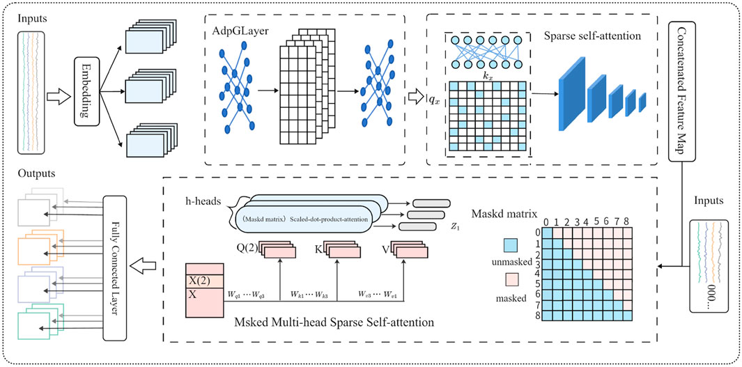
Figure 1. The ACSAformer model consists of three modules: the Adaptive Graph Convolution Module, which dynamically captures data features; the Sparse Self-Attention Module, which reduces computational complexity; and the Masked Multi-Head Sparse Self-Attention Module, which ensures that the model focuses only on valid information during sequence generation while capturing diverse features from the input sequence.

3.1 Problem setting

This study addresses the task of crime spatiotemporal sequence forecasting, which aims to predict the variation of key variables at future time steps based on historical records incorporating both spatial and temporal features. Let the input sequence be denoted as $Z\in {\mathbb{R}}^{L\times d}$, where $L$ represents the length of the time series and $d$ is the feature dimension (e.g., timestamps, latitude, longitude, etc.). The objective is to predict the target variable at a future time step $t+h$, denoted as ${\widehat{Z}}_{t+h}$, using the preceding $L$ time steps. Formally, the task is defined as learning a mapping function $f_{\theta }:Z=\{Z_1,Z_2,\dots ,Z_L\}\to {\widehat{Z}}_{t+h}$, where $Z_i\in {\mathbb{R}}^d$ denotes the feature vector at the $i$-th time step, and $\theta$ represents the model parameters.

3.2 Embedding

The input layer initially combines the spatiotemporal sequence data $Z\in {\mathbb{R}}^{L\times d}$ with positional embeddings $PE$ to obtain the embedded representation $E$, as defined in Equation 1:

$E=Z+PE(1)$

Here, $Z$ represents the raw input sequence, where $L$ is the sequence length and $d$ is the feature dimension. The positional embedding $PE$ is designed to enhance the temporal representation of the input sequence, and is computed using sine and cosine functions as follows Equation 2:

$PE\left(pos,2j\right)=\sin \left(\frac{pos}{2L^{2j/d}}\right),PE\left(pos,2j+1\right)=\cos \left(\frac{pos}{2L^{2j/d}}\right)(2)$

In this formulation, $pos$ denotes the position index within the sequence, $j$ is the embedding dimension index, and $L$ is the input sequence length.

To further enrich temporal modeling, the final input representation integrates three components: positional embeddings, global time stamp embeddings, and scalar-projected values. Specifically, for each time step $t$ and sequence index $x$, the processed input representation $Z^{\text{feed}}[x]$ is computed as follows Equation 3:

$Z^{\text{feed}}\left[x\right]=\alpha \text{Conv}1\text{D}\left(Z_t\left[x\right]\right)+PE\left(L\times \left(t-1\right)+x\right)+{\displaystyle \sum _p}S{E}_p\left(L\times \left(t-1\right)+x\right)(3)$

Here, $\alpha$ is a balancing factor that modulates the scale between scalar projection and embedding components. $\text{Conv}1\text{D}$ denotes the one-dimensional convolution operation applied to the raw input features. $PE(\cdot )$ represents the position embedding function, and $S{E}_p(\cdot )$ is the $p$-th global time stamp embedding. Each $S{E}_p$ corresponds to a specific temporal feature, such as year, month, day, or weekday, allowing the model to explicitly encode multiple temporal granularities.

3.3 Adaptive layer

Crime events are not uniformly distributed across space and time but exhibit pronounced dynamic clustering and dependency structures, which evolve with changes in the social environment. Static graph structures fail to capture such fluid spatial semantics. To address this limitation, we introduce an adaptive graph convolutional layer within the ACSAformer framework. Traditional graph convolutional networks typically assume a fixed graph topology and assign equal importance to neighboring nodes. However, this assumption can dilute critical spatial features and introduce noise from irrelevant connections. In contrast, the adaptive graph convolutional layer dynamically learns the adjacency matrix based on the characteristics of the input sequence, enabling the model to adaptively adjust the connection strength between nodes in response to evolving spatial patterns. The corresponding formula is as follows:

The adaptive graph learning process in ACSAformer begins by generating two trainable parameter matrices, $E_1^x\in {\mathbb{R}}^{n\times d_e}$ and $E_2^x\in {\mathbb{R}}^{n\times d_e}$, where $n$ is the number of nodes and $d_e$ is the embedding dimension. These matrices are used to compute a dynamic adjacency matrix $A^x$ as follows Equation 4:

$A^x=\text{SoftMax}\left(\text{ReLU}\left(E_1^x{\left(E_2^x\right)}^{\top }\right)\right)(4)$

Here, the ReLU function ensures non-negative edge weights, while the SoftMax function is applied row-wise to normalize the adjacency matrix and produce a probabilistic and direction-aware representation of inter-node connections.

After obtaining the adaptive adjacency matrix $A^x$, the node features are updated using a MixHop-based graph convolution strategy, which facilitates information interaction across different variables. Specifically, the input node features ${\mathcal{H}}^x\in {\mathbb{R}}^{n\times d}$ are aggregated through multiple powers of $A^x$, and the output is computed as Equation 5.

${\mathcal{H}}_{\text{out}}^x=\sigma \left(\Vert {‖}_{j\in \mathcal{P}}{\left(A^x\right)}^j{\mathcal{H}}^x\right)(5)$

In this formulation: $\sigma (\cdot )$ is a non-linear activation function (e.g., ReLU or GELU); ${(A^x)}^j$ denotes the $j$-th power of the adjacency matrix, capturing $j$-hop neighbor interactions; $\Vert \Vert$ represents concatenation along the feature dimension.

3.4 Sparse attention

Conventional self-attention mechanisms face high computational complexity and memory overhead when modeling long sequences, which severely limits their efficiency in large-scale spatiotemporal forecasting tasks. To improve computational performance and suppress redundant information in long-sequence processing, ACSAformer incorporates a sparse attention mechanism. This mechanism is based on the principle of probabilistic sparsity, computing dot-product attention only for representative query-key pairs, thereby significantly reducing complexity and enhancing the response to critical features. By reconstructing the attention distribution in a sparse manner, the model becomes more sensitive to key time steps, enabling effective long-range dependency modeling while minimizing redundant computation and memory usage. This strategy not only improves the model’s practicality in resource-constrained environments but also enhances its ability to capture critical events in complex spatiotemporal sequences.

The conventional self-attention mechanism computes interactions between all query-key pairs, resulting in a quadratic computational complexity of $O(L^2)$, where $L$ is the sequence length. Specifically, given a query matrix $Q\in {\mathbb{R}}^{L\times d}$, key matrix $K\in {\mathbb{R}}^{L\times d}$, and value matrix $V\in {\mathbb{R}}^{L\times d}$, the attention output is computed as Equation 6:

$A\left(Q,K,V\right)=\text{Softmax}\left(\frac{Q{K}^{\top }}{\sqrt{d}}\right)V(6)$

This process can also be interpreted from a probabilistic perspective. For the $x$-th query $q_x$, the attention weight over key $k_j$ is defined by an asymmetric kernel smoother Equation 7:

$A\left(q_x,K,V\right)={\displaystyle \sum _j}\frac{k\left(q_x,k_j\right)}{{\sum }_{j}k\left(q_x,k_j\right)}{v}_j={\mathbb{E}}_{p\left(k_j|q_x\right)}\left[v_j\right](7)$

Where $p(k_j|q_x)=\frac{\exp (q_x{k}_j^{\top }/\sqrt{d})}{{\sum }_j\exp (q_x{k}_j^{\top }/\sqrt{d})}$ and $v_j\in V$. While this formulation enables flexible aggregation, its full attention computation incurs substantial memory and runtime costs.

To alleviate this problem, we introduce a sparsity-aware mechanism inspired by the ProbSparse attention framework, which prioritizes query-key pairs based on their attention distribution entropy. Specifically, we define a sparsity score $M(q_x,K)$ for the $x$-th query to quantify the concentration of its attention distribution Equation 8:

$M\left(q_x,K\right)=-\ln \left({\displaystyle \sum _{j=1}^L}\exp \left(\frac{q_x{k}_j^{\top }}{\sqrt{d}}\right)\right)+\frac{1}{L}{\displaystyle \sum _{j=1}^L}\frac{q_x{k}_j^{\top }}{\sqrt{d}}(8)$

A higher $M(q_x,K)$ value indicates a sparser attention distribution, implying stronger preference for a few dominant keys. Based on this measure, we select the top-$u$ most informative queries to participate in attention computation, where Equation 9:

$u=c\cdot \ln L(9)$

Here, $c$ is a sparsity control factor. This logarithmic sparsity strategy reduces the attention complexity from $O(L^2)$ to $O(L\log L)$, while retaining the most impactful query-key interactions. By integrating this mechanism, the model improves both computational efficiency and interpretability in long-sequence forecasting tasks.

4 Experiments

4.1 Datasets

According to the data published by https://www.neighborhoodscout.com/ca/crime, the crime rate in Los Angeles is significantly higher than the national average in the United States. In terms of overall safety, Los Angeles is safer than only approximately 6% of cities nationwide, while the situation in Chicago is even more severe, with a safety score better than just 5% of American cities. The distribution of crime risk across different areas of Los Angeles and Chicago is illustrated in Figure 2. To scientifically evaluate the performance of the ACSAformer model in spatiotemporal crime sequence forecasting, this study collected historical crime records from Los Angeles and Chicago, covering the period from 1 January 2020, to 10 September 2023. During the data preprocessing stage, non-essential attributes were removed to focus on core features, reduce noise, and improve processing efficiency. Subsequently, the Los Angeles dataset was divided into four yearly intervals—corresponding to the years 2020, 2021, 2022, and 2023—each with 2,500 randomly sampled records, resulting in four sub-datasets labeled DS1 through DS4. Additionally, 3,000 records were randomly sampled from the entire Chicago dataset to form an external dataset, DS5. The year-based segmentation of the Los Angeles data ensures that the model learns long-term temporal patterns, while the inclusion of the Chicago dataset facilitates the evaluation of the model’s generalization capability across different urban scenarios. To ensure the scientific rigor and effectiveness of the training process, all datasets were partitioned chronologically into training, validation, and test sets at a ratio of 7:1:2. As shown in Table 1, The dataset is rich in features, including key attributes such as crime date, location, offense type, and case status, providing a robust foundation for assessing the spatiotemporal forecasting performance of the ACSAformer model.

Figure 2

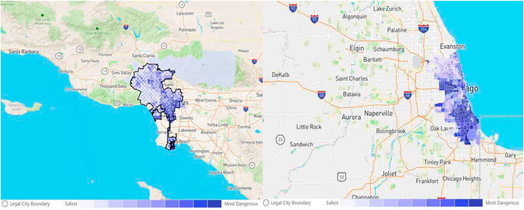
Figure 2. The intensity of the color represents the degree of danger in different regions of Los Angeles and Chicago.

Table 1

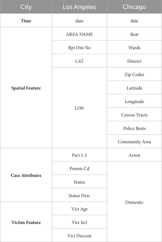
Table 1. Data indicators of Los Angeles and Chicago.

4.2 Implementation details

During the training process, ACSAformer employs Mean Squared Error (MSE) and Mean Absolute Error (MAE) as the primary evaluation metrics and is optimized using the Adam optimizer with an initial learning rate of 0.0001 and a batch size of 16. The model training is prematurely terminated after 10 epochs to prevent overfitting. Each experiment is repeated three times to ensure the stability and reliability of the results. All experiments are conducted within the PyTorch framework and executed on a single NVIDIA RTX 3090 24 GB GPU, ensuring efficient computational support. These implementation details lay a solid foundation for the excellent performance of ACSAformer in crime spatiotemporal sequence forecasting tasks.

4.3 Baselines

In this study, we selected seven spatiotemporal sequence forecasting methods for comparative analysis to comprehensively evaluate the performance of different models in handling complex spatiotemporal data. These methods encompass both mainstream techniques and innovative modeling approaches in the field of spatiotemporal sequence forecasting.

Firstly, models based on the Transformer architecture have been a research hotspot in recent years. We chose LightTS Campos et al. [33] and Autoformer Wu et al. [34] as representatives. LightTS has garnered attention for its efficient computational performance and superior handling of long sequences, while Autoformer has significantly enhanced the model’s ability to capture long- and short-term dependencies in time series data through its innovative self-attention mechanism. Additionally, the classic Transformer [35] model was included in our study. As the pioneering work on self-attention mechanisms, Transformer has laid the foundation for the development of many subsequent models. Its powerful parallel computing capabilities and ability to model long-range dependencies have enabled it to perform outstandingly in various sequence forecasting tasks. Regarding frequency-domain analysis, the FreTS Yi et al. [36] model transforms time series data into the frequency domain for analysis, effectively capturing periodic and seasonal patterns in the data. This approach provides a unique perspective for dealing with time series that exhibit significant periodicity. The FEDformer [37] model, on the other hand, combines Fourier transforms with sparse attention mechanisms. By integrating frequency- and time-domain analyses, FEDformer further enhances the model’s ability to handle complex spatiotemporal sequences. This combination not only leverages the strengths of Fourier transforms in frequency-domain analysis but also effectively reduces computational complexity through sparse attention mechanisms. In terms of multi-scale modeling, the Pyraformer Liu et al. [38] model is based on a pyramid structure and constructs multi-scale representations of time series. This enables it to capture both long- and short-term dependencies simultaneously, providing an effective solution for dealing with data that have complex temporal dependency structures. Finally, the FiLM Zhou et al. [39] model dynamically integrates relationships between multidimensional variables through Feature-wise Linear Modulation. This method excels in handling multivariate time series with complex interactions, effectively capturing the dynamic changes and interactions between variables. By modulating model parameters based on the features of different variables, FiLM can better adapt to complex interaction scenarios.

Through comparative analysis of these seven methods, we aim to provide a comprehensive assessment of model performance in the field of spatiotemporal sequence forecasting and offer valuable references for subsequent research and practical applications.

4.4 Results and analysis

In this study, we employ Mean Squared Error (MSE) and Mean Absolute Error (MAE) as the two primary metrics to evaluate the forecasting accuracy of the ACSAformer model. The calculation formulas are as follows Equations 10, 11:

$\text{MSE}=\frac{1}{n}{\displaystyle \sum _{i=1}^n}{\left(y_x-{\widehat{y}}_i\right)}^2(10)$

$\text{MAE}=\frac{1}{n}{\displaystyle \sum _{i=1}^n}\left|y_x-{\widehat{y}}_i\right|(11)$

In the formulas of MSE and MAE $n$ is the total number of samples. $y_x$ is the true value of the $x$-th sample. ${\widehat{y}}_x$ is the predicted value of the $x$-th sample.

4.4.1 Multivariate result

In this study, Multivariate forecasting refers to the use of multiple input feature variables as joint inputs to the model for learning and predicting the target variable. Specifically, the input features include not only the historical sequence of the victim’s age, but also contextual information associated with each crime record, such as timestamps (e.g., year, month, day) and spatial locations (e.g., latitude, longitude, administrative region). Multivariate modeling enables the extraction of spatiotemporal dependencies and feature interactions within the data, thereby enhancing the accuracy and generalization ability of the prediction. Table 2 summarizes the forecasting performance of all methods across five datasets, highlighting the superior results achieved by ACSAformer. The generalization capability of the models is evaluated by calculating their average rankings across all datasets. Notably, ACSAformer outperforms other models in average ranking, demonstrating the best performance. More specifically, compared to LightTS, ACSAformer reduces the MSE on the DS1 dataset by 17.1%, 21.2%, 12.2%, and 19.9% for forecasting lengths of 12, 36, 58, and 96, respectively, while the MAE is reduced by 8.9%, 11.1%, 6.7%, and 10.4% for the same forecasting lengths. LightTS indirectly captures temporal dependencies through linear or convolutional layers, making it challenging to model complex relationships among multiple variables. In contrast, ACSAformer integrates adaptive graph convolutional layers and ProbSparse self-attention. The adaptive graph convolutional layer dynamically learns the inter-variable dependency structures, enabling the capture of more complex relationships, while the ProbSparse self-attention mechanism employs a sparsity strategy to selectively compute and focus on key time steps, enhancing the ability to capture critical information. The combination of these two components allows ACSAformer to simultaneously capture local details and global dependencies in spatiotemporal sequence, thereby significantly enhancing forecasting accuracy and robustness. Particularly in scenarios with intricate inter-variable relationships, ACSAformer exhibits even more outstanding performance.

Table 2

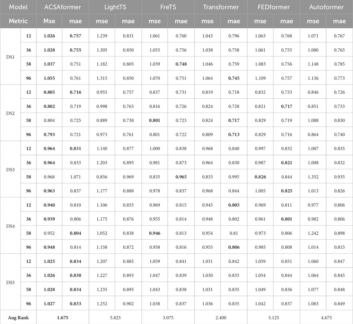
Table 2. Multivariate forecast results with 96 review window and forecasting length12, 36, 58, 96. The best result is represented in bold.

4.4.2 Univariate result

In contrast, Univariate forecasting refers to the use of only the historical sequence of the target variable as the model input, without incorporating any auxiliary features. In this study, the univariate prediction task relies solely on the past values of victim age for modeling and forecasting, omitting contextual information such as time and location. This setup is used to evaluate the model’s basic sequence modeling capability and predictive performance in the absence of external inputs. Table 3 presents the forecasting performance comparison of various methods across five datasets, with ACSAformer demonstrating superior results. The generalization capability of the models is evaluated by calculating their average rankings across all datasets. ACSAformer significantly outperforms other models with the best average ranking, showcasing its exceptional performance. Compared to LightTS, ACSAformer reduces the MSE on the DS1 dataset by 21.1%, 22.5%, 21.8%, and 23.2% for forecasting lengths of 12, 36, 58, and 96, respectively, while the MAE is reduced by 12.6%, 13.8%, 13.2%, and 14.0% for the same forecasting lengths. This significant performance improvement is attributed to the introduction of the adaptive graph convolution module in ACSAformer, which is capable of dynamically learning the dependency structures among variables in time series data. Even in the context of univariate time series forecasting, this module can capture the intrinsic dynamic characteristics of the time series by modeling the implicit relationships between data points, thereby enabling more accurate predictions of future data changes.

Table 3

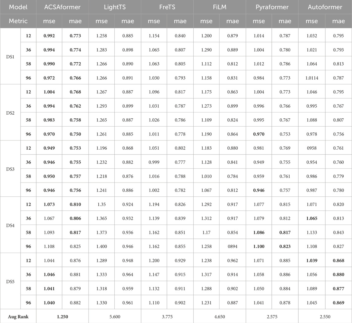
Table 3. Univariate forecast results with 96 review window and forecasting length12, 36, 58, 96. The best result is represented in bold.

4.4.3 Ablation study

Table 4 presents the ablation study results of the ACSAformer model on five datasets. We designed five ablation methods to validate the effectiveness of each module in the model. The specific implementations are as follows:

$•$ O-C: The adaptive graph convolutional layer is removed from the model.

$•$ T-ST: The sparse attention mechanism is replaced with the traditional self-attention mechanism.

$•$ O-C/T-ST: Both the adaptive graph convolutional layer is removed and the sparse attention mechanism is replaced with the traditional self-attention mechanism.

Table 4

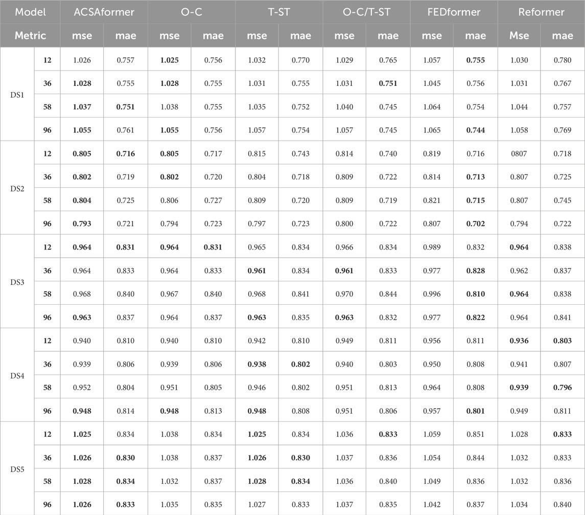
Table 4. Ablation analysis of five datasets. Results represent the average error of forecasting length 12,36,58,96, with the best performance highlighted in bold black.

Through the analysis of the experimental results, we draw the following conclusions:

$•$ Importance of the Adaptive Graph Convolutional Layer: After removing the adaptive graph convolutional layer, the model performance significantly declines. This indicates that adaptively learning inter-sequence correlations is crucial for multivariate spatiotemporal sequence forecasting tasks.

$•$ Improvement of the Sparse Attention Mechanism: Compared with the results of the trans-attention variant, the sparse attention mechanism outperforms the traditional self-attention mechanism in capturing global features, thereby enhancing the model’s performance.

$•$ Synergistic Effect of the Adaptive Graph Convolutional Layer and Sparse Attention: The results of the o-AdapGlyer and trans-attention variant further validate that the combination of the adaptive graph convolutional layer and the sparse attention mechanism significantly improves the model’s performance.

$•$ Superiority of the Sparse Attention Mechanism: Compared with FEDformer’s frequency-domain decomposition + hybrid attention mechanism and Reformer’s Locality-Sensitive Hashing (LSH) attention + chunked attention + reversible layer mechanism, ACSAformer’s sparse attention mechanism demonstrates superior performance in capturing global features, highlighting its advantage in complex spatiotemporal sequence modeling.

In summary, the ablation experiments confirm the effectiveness of the adaptive convolutional layer and the sparse attention mechanism. By effectively combining these two components, ACSAformer significantly enhances the performance of multivariate spatiotemporal sequence forecasting.

5 Discusion

5.1 Efficiency evaluation

Figure 3 illustrates the speed comparison of ACSAformer, CrossFormer, Autoformer, Pyraformer, and FEDformer on the DS1 and DS4 datasets under different forecasting steps (12, 36, 58, 96). The computational efficiency (speed) of each model was evaluated by measuring the time required to complete one iteration (iter), expressed in milliseconds. The models differ in their attention mechanisms: CrossFormer, based on cross-attention, captures multi-scale dependencies through cross-feature interactions, with a complexity of O (L²). Autoformer combines self-attention with a sequence decomposition architecture, achieving a complexity of O (L²), making it suitable for handling complex temporal patterns. Pyraformer employs a pyramidal attention mechanism, hierarchically modeling multi-scale temporal dependencies, with a complexity of O (L log L). FEDformer leverages frequency-domain attention, enhancing temporal modeling through frequency-domain transformations, with a complexity of O (L²). In contrast, ACSAformer utilizes a sparse attention mechanism, selectively computing key time steps, significantly reducing computational complexity from O (L²) to O (L log L), thereby minimizing computational and memory overhead and demonstrating superior speed. As the forecasting steps increase, the speed of all models decreases, but ACSAformer remains efficient even for long forecasting steps 96, showcasing its robustness. In complex scenarios, its efficiency and stability make it a preferred model for spatiotemporal sequence forecasting.

Figure 3

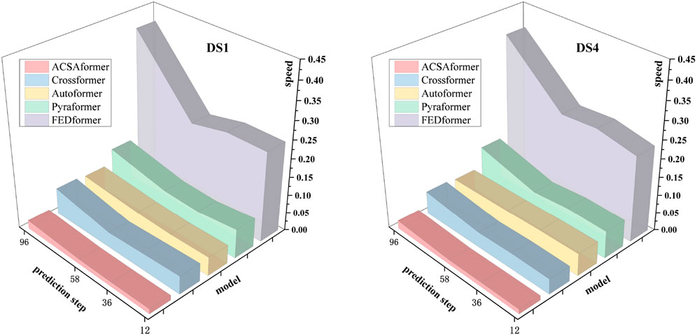
Figure 3. In this experiment, five distinct models were employed to perform forecastings on the DS1 and DS4 datasets. The input length was fixed at 96, with forecasting lengths set to 12, 36, 58, and 96.

5.2 Model’s ability to resist noise

In this study, we conducted a comprehensive assessment of the robustness of the ACSAformer model in resisting noise interference in crime spatiotemporal sequence data. Considering that crime spatiotemporal sequence data are susceptible to multiple complex noise sources, we paid special attention to the model’s performance in complex environments. As shown in Figure 4, we introduced 50% and 100% Gaussian white noise into the DS1 and DS4 datasets, respectively, to simulate the diverse relationships between signals and noise in real-world scenarios, making the experimental environment more realistic. The results show that the ACSAformer model performs outstandingly in handling noisy data and has significant advantages over other models. The sparse attention mechanism of ACSAformer is capable of capturing global dependencies in long sequences, while the adaptive graph convolutional layer excels at extracting local spatial features. The integration of these two components enables the model to effectively perform feature extraction at both global and local levels, thereby significantly enhancing its prediction accuracy and robustness. This ensures that the model maintains high prediction accuracy even under noisy conditions.

Figure 4

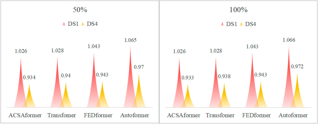
Figure 4. 50% and 100% indicating the degree of noise impact on data. Prediction Results Reveal the Noise Resistance Performance of Different Models on DS1 and DS4 Datasets with Input Length 96 and prediction step 36.

5.3 Hyperparameter experiment

5.3.1 Review window

In general, the size of the review window influences the types of dependencies that a model can learn from historical information. A proficient spatiotemporal sequence forecasting model should accurately capture dependencies over extended review windows, leading to improved results. In a previous study, it was demonstrated that Transformer-based models tend to exhibit significant fluctuations in their performance, resulting in either an overall decline in performance or reduced stability as the review window lengthens. As illustrated in Figure 5 We conducted a similar analysis on the DS1 and DS4 datasets, employing four review windows, namely, 12, 36, 58, 96, to predict the values for the subsequent 12 time steps. Mean Squared Error (MSE) and Mean Absolute Error (MAE) were selected as the evaluation metrics. As shown in the figure, ACSAformer outperformed other models in the review window experiments, with significantly lower MSE and MAE values on both DS1 and DS4 datasets. Notably, it maintained low error rates even at longer forecasting steps (e.g., 96), demonstrating its strong capability in modeling long-range dependencies. Autoformer and Transformer showed moderate performance, while FreTS and SCINet exhibited larger errors at certain forecasting steps, particularly under longer forecasting horizons. Overall, as the forecasting step increased, the errors of all models showed an upward trend. However,For each output feature channel, the adaptive graph convolutional layer dynamically adjusts the convolution kernel based on the feature differences between neighboring points. This mechanism allows the convolution kernel to adaptively adjust according to changes in the input features, thereby more accurately capturing local geometric structures. The dynamic adjustment mechanism enhances the model’s generalization ability and prediction accuracy when processing complex data the robustness and generalization ability of ACSAformer made it particularly outstanding in complex data scenarios.

Figure 5

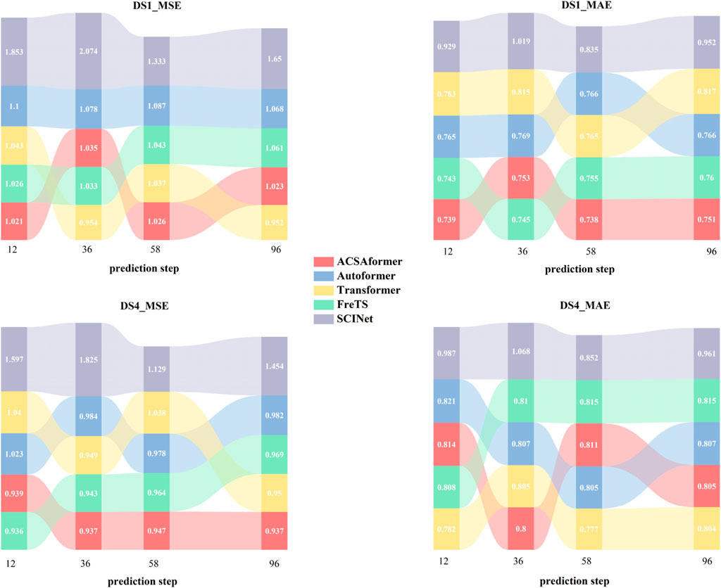
Figure 5. DS1 and DS4 datasets forecastings for 12 time steps withdifferent review windows. We use four other models for comparison.

5.3.2 Dropout

In spatiotemporal sequence forecasting, the dropout rate is a crucial hyperparameter. By randomly deactivating neurons during training, it reduces the model’s reliance on specific features, thereby enhancing generalization ability. Figure 6 presents the ACSAformer model’s performance under various dropout rates (ranging from 0.05 to 0.25) across the DS1 and DS4 datasets, with respect to the forecasting horizon on Mean Squared Error (MSE) and Mean Absolute Error (MAE). The experimental results indicate that the dropout rate has a certain impact on the model’s error metrics, as there are differences in the MSE and MAE curves under different dropout rates, demonstrating the model’s sensitivity to the dropout rate. Moreover, as the forecasting step increases, both MSE and MAE exhibit a slight upward trend, suggesting a decrease in predictive accuracy with an extended forecasting horizon. Nonetheless, the ACSAformer model demonstrates commendable stability and generalization capability when dealing with different dropout rates and forecasting steps.

Figure 6

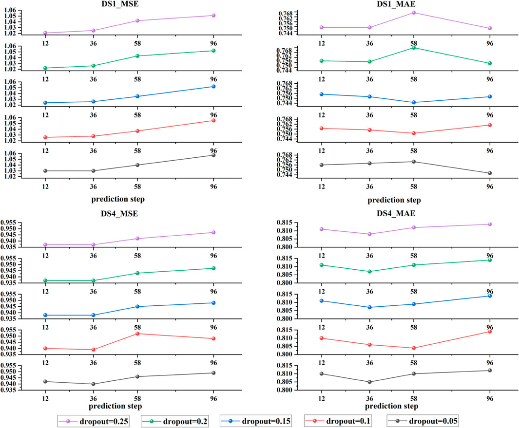
Figure 6. The figure illustrates the variations in Mean Squared Error (MSE) and Mean Absolute Error (MAE) for two distinct datasets, DS1 and DS4, under different dropout parameters.

5.3.3 Batch-size

In spatiotemporal sequence forecasting, batch size is a pivotal hyperparameter influencing computational efficiency, convergence behavior, and generalization capability. Smaller batches facilitate escaping local minima but may induce training instability, whereas larger batches yield more stable gradients and expedite convergence, albeit potentially diminishing generalization. Figure 7 presents the Mean Squared Error (MSE) and Mean Absolute Error (MAE) of the ACSAformer model under varying batch sizes (ranging from 4 to 20) across the DS1 and DS4 datasets as the forecasting horizon changes. The experimental results indicate that batch size has a limited impact on the model’s error metrics, as the MSE and MAE curves are relatively close across different batch sizes, demonstrating the model’s robustness to variations in batch size. However, as the forecasting step increases, both MSE and MAE exhibit a slight upward trend, suggesting a decrease in predictive accuracy with an extended forecasting horizon. Nonetheless, the ACSAformer model demonstrates commendable stability and generalization capability when dealing with different batch sizes and forecasting steps.

Figure 7

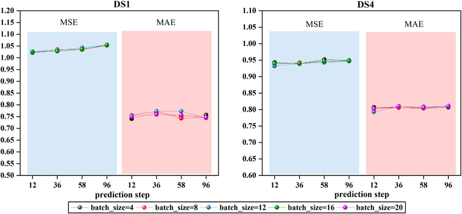
Figure 7. The figure illustrates the variations in Mean Squared Error (MSE) and Mean Absolute Error (MAE) for two distinct datasets, DS1 and DS4, under different batch_size parameters.

5.3.4 Encoder layer

The number of encoder layers plays a crucial role in spatiotemporal sequence modeling. Appropriately increasing the depth can enhance the model’s ability to capture complex temporal dependencies, particularly in long-sequence forecasting tasks. However, excessively deep architectures may lead to training instability, increased risk of overfitting, and decreased inference efficiency. As illustrated in Figure 8, we analyze the impact of different encoder depths on prediction performance using the DS1 and DS4 datasets. The vertical axis represents the number of encoder layers, and each heatmap cell denotes the average evaluation score across four prediction lengths (12, 36, 58, 96), thereby mitigating the randomness introduced by individual step sizes. From the MSE heatmap, we observe a slight increase in error on DS1 as the number of layers grows (from 1.036 to 1.046), indicating that deeper encoders do not significantly improve modeling capability for this dataset. In contrast, performance on DS4 remains stable (ranging from 0.945 to 0.954), suggesting better robustness and generalization. A similar trend is seen in the MAE heatmap: DS1 shows minor fluctuations, while DS4 maintains consistent results across all depths (0.806–0.808). Notably, the model achieves optimal performance with the default single-layer encoder (layer = 1), demonstrating the high efficiency of the proposed architecture. This lightweight configuration not only reduces training and inference costs but also enhances the model’s stability and adaptability in practical applications.

Figure 8

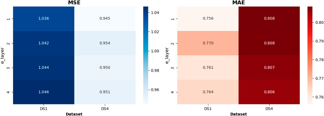
Figure 8. With the review window length set to 96, experiments were conducted under four prediction horizons: 12, 36, 58, and 96. In the heatmap, the color intensity of each block represents the average of the Mean Squared Error (MSE) and Mean Absolute Error (MAE) obtained across these four prediction settings.

5.3.5 Learning rate

As a key hyperparameter in deep learning models, the learning rate significantly affects both the convergence speed and the final performance. An excessively small learning rate may lead to slow convergence and difficulty in escaping local minima, while an overly large learning rate can cause gradient oscillations, resulting in unstable training and degraded performance. As shown in Figure 9, we evaluate the impact of four different learning rate settings (0.0001, 0.0003, 0.0005, and 0.001) on model performance using MSE and MAE metrics across the DS1 and DS4 datasets, in order to assess the model’s robustness and sensitivity to this parameter. The figure illustrates the prediction errors under different learning rates, where the darker segments represent MSE and the lighter segments indicate MAE. The height of each bar corresponds to the magnitude of the error. On the DS1 dataset, increasing the learning rate from the default value of 0.0001 leads to a noticeable rise in both MSE and MAE, suggesting that a larger learning rate may impair the model’s ability to fit local patterns, thus reducing prediction accuracy. In contrast, the performance on the DS4 dataset remains relatively stable across different learning rates, particularly in terms of MSE, reflecting stronger generalization and robustness. Notably, the model achieves the best performance on both datasets when the learning rate is set to the default value of 0.0001, further confirming the validity and practicality of this parameter choice. In summary, while the model demonstrates consistent robustness across different learning rates, its optimal performance under the 0.0001 setting highlights the scientific rationale and effectiveness of this configuration for the current task.

Figure 9

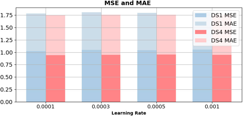
Figure 9. Under a review window length of 96, experiments were conducted with four prediction lengths: 12, 36, 58, and 96. The height of each color block in the figure represents the average Mean Squared Error (MSE) and Mean Absolute Error (MAE) across these four prediction settings.

5.3.6 Embedding dimension

Embedding dimension is a critical factor influencing the performance of spatiotemporal sequence modeling. A dimension that is too low may result in insufficient feature representation, making it difficult to capture complex temporal dependencies; conversely, an excessively high dimension can introduce redundant information and increase model complexity, thereby impairing generalization and stability. To comprehensively assess the impact of this parameter, we evaluate four embedding dimension settings (64, 256, 512, and 1024) on the DS1 and DS4 datasets, as shown in Figure 10, using MSE and MAE as evaluation metrics. The figure presents the average MSE and MAE values computed across four prediction horizons under each embedding dimension. These results are visualized in radar charts for the two datasets, providing an intuitive overview of how embedding size affects overall model performance. From the radar chart of DS1, it can be observed that the default embedding size of 256 yields relatively better performance on both MSE and MAE. However, when the dimension increases to 1024, the model performance degrades slightly, suggesting that high-dimensional embeddings may lead to overfitting due to redundant information. In contrast, the DS4 results exhibit smaller fluctuations across different dimensions, indicating a more stable performance and stronger robustness. In summary, an embedding dimension of 256 provides a good balance between accuracy and stability across both datasets, confirming the effectiveness of this default setting in the current task. These findings also suggest that properly controlled embedding sizes can enhance model prediction, while both under- and over-dimensioned configurations may have adverse effects on performance.

Figure 10

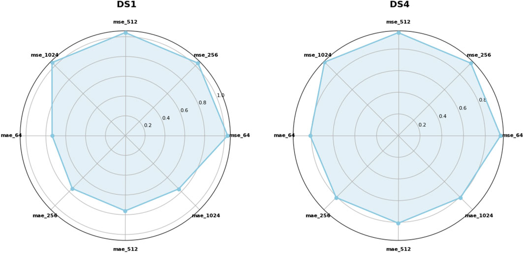
Figure 10. With the review window length fixed at 96, we configured four prediction horizons: 12, 36, 58, and 96. In the figure, each vertex represents the average of the Mean Squared Error (MSE) and Mean Absolute Error (MAE) obtained across these four prediction settings.

6 Conclusion

In this study, we propose an innovative spatio - temporal sequence prediction framework named ACSAformer, aiming to overcome the limitations of existing deep learning models in handling complex spatio - temporal data. ACSAformer combines a sparse attention mechanism and knowledge distillation operations and employs a probabilistic method to screen out important attention weights for calculation, successfully reducing the computational complexity of the model to $O(L\log L)$. Moreover, by applying one - dimensional convolution, the ELU activation function, and max - pooling operations for feature downsampling, ACSAformer significantly enhances the model’s ability to capture key features. This series of improvements enables ACSAformer to perform excellently in crime spatio - temporal sequence prediction tasks.

Furthermore, ACSAformer introduces an adaptive graph convolutional layer, which dynamically adjusts the size, shape, or parameters of the convolutional kernel to enhance the model’s ability to capture the complex relationships and dynamic correlations among different features. This innovation not only improves the generalization ability of the model but also further enhances the prediction accuracy.

Through extensive experiments on five real - world datasets, ACSAformer demonstrates its significant advantages in prediction accuracy, generalization ability, and robustness. Overall, the application of ACSAformer in spatio - temporal sequence prediction tasks has achieved certain results, laying a foundation for further optimization and expansion in the future.

Data availability statement

The original contributions presented in the study are publicly available. This data can be found here: https://figshare.com/articles/dataset/SAformer_data/28604453.

Author contributions

ZQ: Conceptualization, Formal Analysis, Investigation, Methodology, Writing – original draft. BW: Investigation, Methodology, Software, Writing – original draft. CG: Data curation, Formal Analysis, Investigation, Methodology, Validation, Visualization, Writing – original draft. FZ: Conceptualization, Investigation, Project administration, Resources, Supervision, Writing – review and editing. WQ: Conceptualization, Project administration, Resources, Supervision, Validation, Writing – review and editing. QZ: Resources, Validation, Writing – review and editing.

Funding

The author(s) declare that no financial support was received for the research and/or publication of this article.

Conflict of interest

The authors declare that the research was conducted in the absence of any commercial or financial relationships that could be construed as a potential conflict of interest.

Generative AI statement

The author(s) declare that no Generative AI was used in the creation of this manuscript.

Publisher’s note

All claims expressed in this article are solely those of the authors and do not necessarily represent those of their affiliated organizations, or those of the publisher, the editors and the reviewers. Any product that may be evaluated in this article, or claim that may be made by its manufacturer, is not guaranteed or endorsed by the publisher.

References

1. Mohler GO, Short MB, Brantingham PJ, Schoenberg FP, Tita GE. Randomized controlled field trials of predictive policing. J Quantitative Criminology (2018) 34:751–72. doi:10.1007/s10940-017-9368-0

CrossRef Full Text | Google Scholar

2. Xun G, Jha K, Gopalakrishnan V, Li Y, Zhang A. Generating medical hypotheses based on evolutionary medical concepts. In: 2017 IEEE International conference on data mining (ICDM) (IEEE) (2017). p. 535–44.

Google Scholar

3. Wang S, Wang M, Liu Y. Access to urban parks: comparing spatial accessibility measures using three gis-based approaches. Comput Environ Urban Syst (2021) 90:101713. doi:10.1016/j.compenvurbsys.2021.10113

CrossRef Full Text | Google Scholar

4. Wang X, Zhang Y, Liu Z. Application of arma model in short-term crime prediction. J Comput Social Sci (2021) 4:189–202. doi:10.1007/s42286-021-00093-2

CrossRef Full Text | Google Scholar

5. Zaki M. Hybrid approach based on ARIMA and artificial neural networks for crime series forecasting. Universiti Teknologi Malaysia (2014).

Google Scholar

6. Soares FA, Silveira TB, Freitas HC. Hybrid approach based on sarima and artificial neural networks for knowledge discovery applied to crime rates prediction. ICEIS (2020)(1) 407–15. doi:10.5220/0009412704070415

CrossRef Full Text | Google Scholar

7. Su L, Xiong L, Yang J. Multi-attn bls: multi-head attention mechanism with broad learning system for chaotic time series prediction. Appl Soft Comput (2023) 132:109831. doi:10.1016/j.asoc.2022.109831

CrossRef Full Text | Google Scholar

8. Hossain S, Abtahee A, Kashem I, Hoque MM, Sarker IH. Crime prediction using spatio-temporal data. In: Computing science, communication and security: first international conference, COMS2 2020, Gujarat, India, march 26–27, 2020, revised selected papers 1. Springer (2020). p. 277–89.

Google Scholar

9. Li Z, Huang C, Xia L, Xu Y, Pei J. Spatial-temporal hypergraph self-supervised learning for crime prediction. In: 2022 IEEE 38th international conference on data engineering (ICDE) (2022). p. 2984–96. doi:10.1109/ICDE53745.2022.00269

CrossRef Full Text | Google Scholar

10. Vaswani A, Shazeer N, Parmar N, Uszkoreit J, Jones L, Gomez AN, et al. Attention is all you need. Adv Neural Inf Process Syst (2017) 30. doi:10.5555/3295222.3295349

CrossRef Full Text | Google Scholar

11. Wang X, Xue K, Liu X. Research on fault handling of digital twin power data communication network based on gis geographic information. In: 2023 35th Chinese control and decision conference (CCDC) (2023). p. 1332–6. doi:10.1109/CCDC58219.2023.10326636

CrossRef Full Text | Google Scholar

12. Zhou H, Zhang S, Peng J, Zhang S, Li J, Xiong H, et al. Informer: beyond efficient transformer for long sequence time-series forecasting. Proc AAAI Conf Artif intelligence (2021) 35:11106–15. doi:10.1609/aaai.v35i12.17325

CrossRef Full Text | Google Scholar

13. Kipf TN, Welling M. Semi-supervised classification with graph convolutional networks. arXiv preprint arXiv:1609.02907 (2016).

Google Scholar

14. Brandon W, Driscoll B, Dai F, Berkow W, Milano M. Better defunctionalization through lambda set specialization. Proc ACM Program Lang (2023) 7:977–1000. doi:10.1145/3591260

CrossRef Full Text | Google Scholar

15. Hu K, Long Z, Li W, Fan J, Liu S, Zhou F, et al. Research on measuring method of power frequency superimposed impulse voltage. In: 2022 IEEE 5th international electrical and energy conference (CIEEC) (2022). p. 4283–6. doi:10.1109/CIEEC54735.2022.9846310

CrossRef Full Text | Google Scholar

16. Wang S, Wang M, Liu Y. Access to urban parks: comparing spatial accessibility measures using three gis-based approaches. Comput Environ Urban Syst (2021) 90:101713. doi:10.1016/j.compenvurbsys.2021.101713

CrossRef Full Text | Google Scholar

17. Saha M, Santara A, Mitra P, Chakraborty A, Nanjundiah RS. Prediction of the indian summer monsoon using a stacked autoencoder and ensemble regression model. Int J Forecast (2021) 37:58–71. doi:10.1016/j.ijforecast.2020.03.001

CrossRef Full Text | Google Scholar

18. Ilhan F, Tekin SF, Aksoy B. Spatio-temporal crime prediction with temporally hierarchical convolutional neural networks. In: 2020 28th signal processing and communications applications conference (SIU) (2020). p. 1–4. doi:10.1109/SIU49456.2020.9302169

CrossRef Full Text | Google Scholar

19. Kipf TN, Welling M. Semi-supervised classification with graph convolutional networks. arXiv preprint arXiv:1609.02907 (2016).

Google Scholar

20. Vaswani A, Shazeer N, Parmar N, Uszkoreit J, Jones L, Gomez AN, et al. Attention is all you need. Adv Neural Inf Process Syst (2017) 30. doi:10.5555/3295222.3295349

CrossRef Full Text | Google Scholar

21. Xiao Y, Xia K, Yin H, Zhang YD, Qian Z, Liu Z, et al. Afstgcn: prediction for multivariate time series using an adaptive fused spatial-temporal graph convolutional network. Digital Commun Networks (2024) 10:292–303. doi:10.1016/j.dcan.2022.6.019

CrossRef Full Text | Google Scholar

22. Dong Z, Mnih A, Tucker G. Disarm: an antithetic gradient estimator for binary latent variables. Adv Neural Inf Process Syst (2020) 33:18637–47. doi:10.5555/3495724.3497289

CrossRef Full Text | Google Scholar

23. Raspopov VY, Alaluev R, Shepilov S, Likhosherst V. Gyrostabilizer with an increased controlled precession rate based on a gyroscope with a spherical ball bearing suspension. In: 2021 28th saint petersburg international conference on integrated navigation Systems (ICINS) (2021). p. 1–4. doi:10.23919/ICINS43216.2021.9470819

CrossRef Full Text | Google Scholar

24. Takayama N, Arai S. Objective weight interval estimation using adversarial inverse reinforcement learning. IEEE Access (2023) 11:58532–8. doi:10.1109/ACCESS.2023.3281593

CrossRef Full Text | Google Scholar

25. Juwara L, El-Hussuna A, El Emam K. An evaluation of synthetic data augmentation for mitigating covariate bias in health data. Patterns (2024) 5:100946. doi:10.1016/j.patter.2024.100946

PubMed Abstract | CrossRef Full Text | Google Scholar

26. Xiao Y, Xia K, Yin H, Zhang YD, Qian Z, Liu Z, et al. Afstgcn: prediction for multivariate time series using an adaptive fused spatial-temporal graph convolutional network. Digital Commun Networks (2024) 10:292–303. doi:10.1016/j.dcan.2022.06.019

CrossRef Full Text | Google Scholar

27. Li L, Tang M, Yang Z, Hu J, Zhao M. Spatio-temporal adaptive convolution and bidirectional motion difference fusion for video action recognition. Expert Syst Appl (2024) 255:124917. doi:10.1016/j.eswa.2024.124917

CrossRef Full Text | Google Scholar

28. Zhu T, Li L, Yang J, Zhao S, Liu H, Qian J. Multimodal sentiment analysis with image-text interaction network. IEEE Trans Multimedia (2023) 25:3375–85. doi:10.1109/TMM.2022.3160060

CrossRef Full Text | Google Scholar

29. Spinelli I, Scardapane S, Uncini A. Adaptive propagation graph convolutional network. IEEE Trans Neural Networks Learn Syst (2020) 32:4755–60. doi:10.1109/tnnls.2020.3025110

PubMed Abstract | CrossRef Full Text | Google Scholar

30. Bai L, Yao L, Li C, Wang X, Wang C. Adaptive graph convolutional recurrent network for traffic forecasting. Adv Neural Inf Process Syst (2020) 33:17804–15. doi:10.5555/3495724.3497218

CrossRef Full Text | Google Scholar

31. Chen S, Gao J, Reddy S, Berseth G, Dragan AD, Levine S. Asha: assistive teleoperation via human-in-the-loop reinforcement learning. Int Conf Robotics Automation (Icra) (2022) 7505–12. doi:10.1109/ICRA46639.2022.9812442

CrossRef Full Text | Google Scholar

32. Guo HX, Hong TT, Zhang YW. Path planning simulation and research of mobile robot in static environment based on genetic algorithm. In: 2023 8th international conference on automation, control and robotics engineering (CACRE) (2023). p. 226–30. doi:10.1109/CACRE58689.2023.10208742

CrossRef Full Text | Google Scholar

33. Campos D, Zhang M, Yang B, Kieu T, Guo C, Jensen CS. Lightts: lightweight time series classification with adaptive ensemble distillation. Proc ACM Manag Data (2023) 1:1–27. doi:10.1145/3589316

CrossRef Full Text | Google Scholar

34. Wu H, Xu J, Wang J, Long M. Autoformer: decomposition transformers with auto-correlation for long-term series forecasting. Adv Neural Inf Process Syst (2021) 34:22419–30.

Google Scholar

35. Vaswani A, Shazeer N, Parmar N, Uszkoreit J, Jones L, Gomez AN, et al. Attention is all you need. Adv Neural Inf Process Syst (2017) 30. doi:10.5555/3295222.3295349

CrossRef Full Text | Google Scholar

36. Yi K, Zhang Q, Fan W, Wang S, Wang P, He H, et al. Frequency-domain mlps are more effective learners in time series forecasting. Adv Neural Inf Process Syst (2023) 36:76656–79.

Google Scholar

37. Zhou T, Ma Z, Wen Q, Wang X, Sun L, Jin R. Fedformer: frequency enhanced decomposed transformer for long-term series forecasting. In: International conference on machine learning (PMLR) (2022). p. 27268–86.

Google Scholar

38. Liu S, Yu H, Liao C, Li J, Lin W, Liu AX, et al. Pyraformer: low-complexity pyramidal attention for long-range time series modeling and forecasting. In: # PLACEHOLDER_PARENT_METADATA_VALUE# (2022).

Google Scholar

39. Zhou T, Ma Z, Wen Q, Sun L, Yao T, Yin W, et al. Film: frequency improved legendre memory model for long-term time series forecasting. Adv Neural Inf Process Syst (2022) 35:12677–90.

Google Scholar

40. Qin Z, Wei B, Gao C, Chen X, Zhang H, Un C. Sfdformer: a frequency-based sparse decomposition transformer for air pollution time series prediction. Front Environ Sci (2022) 13(?):1549209. doi:10.3389/fenvs.2025.1549209

CrossRef Full Text | Google Scholar

41. Message from the doctoral forum chairs. 2022 52nd annual IEEE/IFIP international conference on dependable Systems and networks - supplemental volume (DSN-S) (2022), 13. doi:10.1109/DSN-S54099.2022.00009

CrossRef Full Text | Google Scholar