Prediction of bundle-conductor ampacity based on transformer-LSTM

The traditional method cannot meet the demand of new power system for dynamic regulation of transmission lines. In order to solve this defect, based on finite element simulation and neural network, an overhead bundle-conductor dynamic bundle-conductor ampacity prediction method is proposed in this paper. Considering the four bundle- JL/G1A-400/35 steel-core aluminum stranded wire, the three-dimensional electric-thermal-fluid coupling model of the conductor is established by using the synergistic optimization of transformer and long-short-term memory neural network (LSTM). The results show that the mean square error and average absolute error of the proposed model are 31.14 and 6.93, respectively. Compared with the bidirectional long and short-term memory network (BiLSTM), the mean square error and average absolute error are reduced by 74.55% and 7.35%, respectively. The maximum improvement of load capacity prediction margin is 10.04%. It can effectively tap the dynamic potential of transmission lines, and provide technical support for real-time scheduling of smart grid.

1 Introduction

The rapid decarburization of global energy systems is driving increased demand for dynamic regulation capacity in renewable-dominated transmission networks [1, 2]. As the central infrastructure of ultra-high voltage (UHV) transmission networks, dynamic prediction of the real-time carrying capacity has emerged as a critical technological challenge for ensuring safe, economic grid operations and efficient utilization of renewable energy [3, 4].

The prediction methodologies of bundle-conductor ampacity are traditionally classified into two principal categories: physics-based mechanistic models and data-driven approaches, with pronounced disparities observed in their theoretical rigor, computational performance, and versatility across application scenarios. Among the prediction methods based on physical mechanisms, the conventional Static Thermal Rating (STR) method is grounded in the steady-state thermal equilibrium equation. The conductor current-carrying capacity is derived through exclusive reliance on prescribed environmental variables, such as maximum ambient temperature and negligible wind conditions [5]. Despite its simplicity and computational efficiency, the STR method underestimates conductor capacity due to reliance on fixed conservative assumptions (e.g., static meteorological thresholds) rather than real-time environmental conditions. It fails to adapt to load fluctuations from intermittent renewables, limiting its relevance in dynamic power systems. Especially in the high penetration scenarios of fluctuating power sources, such as wind power and photovoltaic, the frequently of transmission line faces the challenges of alternating short-term overloads and long-term low loads. As a result, the traditional static method cannot mitigate localized conductor overheating risks and fully exploit transmission capacity, making them incompatible with modern power systems requiring precise load flow prediction under dynamic conditions. To address this issue, another prediction method is proposed. It is based on physical mechanism, called as dynamic thermal rating (DTR) [6]. By using conductor-mounted sensors to monitor temperature, wind speed and solar irradiance, and combining real-time data with heat transfer models, DTR dynamically adjusts line capacity [7]. Its prediction accuracy is significantly improved. As evaluated in [8], the transmission line capacity obtained by DTR is enhanced by 5%–20% compared by STR. A stochastic transmission expansion planning model considering DTR uncertainty is proposed in [9]. It can optimize the deployment of new lines with DTR systems, and uses DTR to improve line capacity and reduce investment in new lines.

The data-driven load capacity prediction methods have gradually become a research hotspot. Traditional machine learning algorithms, such as Support Vector Regression (SVR) and Random Forest (RF), combine historical meteorological data and load data to train models. They are able to respond quickly to changes in meteorological parameters by mining non-linear relationships in historical data. The 15-min conductor load variation is predicted in [10] using Random Forest and Quantile Random Forest combined with numerical weather data. However, the model generalization is limited by the quality and scale of training data, and long-term temporal dependencies are not effectively captured. In [11], a probabilistic machine learning method for dynamic line rating is proposed. The weather observations are utilized to improve short-term prediction accuracy, and two adaptive strategies are developed to optimize the trade-off between capacity enhancement and risk mitigation. Nevertheless, the model shows inadequate adaptation to extreme events like sustained high temperatures, potentially causing DTR prediction failures. Deep learning has been introduced to load forecasting due to its superior time-series modeling capability, where bi-directional long and short term memory network (BiLSTM) effectively captures the temporal dependencies of meteorological parameters through its bidirectional processing mechanism. An auto-encoder (AE) and BiLSTM are integrated in [12] to address the problem of encountering network attacks in load forecasting. However, larger training datasets and additional conductor-mounted weather sensors are required by this approach. In addition, many studies ignore the influence of the electromagnetic-thermal-fluid coupling effect between multiple conductors of bundle-conductor on data characteristics. It limits the applicability under complex working conditions.

To address the above problem, a dynamic bundle-conductor ampacity prediction method for overhead bundle-conductors based on finite element simulation and neural network is proposed. It does not require the installation of meteorological sensors. Firstly, a three-dimensional coupled electro-thermal-fluid finite element model of bundle-conductor is developed by using COMSOL. This model addresses the oversimplification of boundary conditions in conventional approaches under extreme meteorological conditions. Secondly, long-short-term memory (LSTM) model is developed to predict the overhead conductor capacity without meteorological sensors, combining the LSTM temporal modeling with the global attention of transformer for enhanced feature extraction. Finally, the accuracy of the model is demonstrated by comparing with the rest of the load capacity prediction models. The gain effect on the grid security margin and new energy consumption is quantified by comparing with the traditional load capacity calculation methods.

2 Methodology for bundle-conductor ampacity

2.1 Heat balance equation for bundle-conductors

The dynamic equilibrium between joule heating and environmental heat dissipation during operation are characterized by the thermal balance equation of overhead bundle conductors [13]. The fundamental equation serves as the theoretical basis for both capacity calculation and transmission line safety assessment. Neglecting the hysteresis loss, evaporative heat dissipation and corona heating, the steady state heat balance equation of bundle-conductor can be expressed by Equation 1:

$q_{\mathrm{c}}+q_{\mathrm{r}}=q_{\mathrm{s}}+I^{2}R\left(T_C\right)(1)$

where q_c is the conductor convection heat dissipation power; q_r is the conductor radiation heat dissipation power; q_s is the conductor sunshine heat absorption power. I is the conductor current, T_c is the temperature of the conductor and R (T_c) is the AC resistance of the conductor at T_c.

Conductor convection heat dissipation includes the natural convection and forced convection. The power of natural convection heat dissipation can be expressed by Equation 2:

$q_{c1}=0.0205{\rho }_f^{0.5}{D}^{0.75}{\left(T_c-T_a\right)}^{1.25}(2)$

where T_a is the ambient temperature, and D is the outer diameter of the wire. The power of forced convection heat dissipation at low air velocity can be expressed by Equation 3:

$q_{c2}=\left[1.01+0.0372{\left(\frac{D{\rho }_f{V}_w}{{\mu }_f}\right)}^{0.52}\right]k_f{K}_{angle}\left(T_c-T_a\right)(3)$

where K_angle is the wind direction coefficient, which can be calculated by Equation 4:

$K_{angle}=1.194-\cos \phi +0.194\cos \left(2\phi \right)+0.368\sin \left(2\phi \right)(4)$

where φ is the angle between the wind direction and the axis of the conductor.

The power of forced convection heat dissipation at high air velocity can be expressed by Equation 5:

$q_{c3}=0.0119{\left(\frac{D{\rho }_f{V}_w}{{\mu }_f}\right)}^{0.6}{k}_f{K}_{angle}\left(T_c-T_a\right)(5)$

The convective heat dissipation power q_c can be determined by Equation 6:

$q_c=\max \left\{q_{c_1},q_{c_2},q_{c_3}\right\}(6)$

The radiant heat dissipation power of the conductor is defined by Equation 7:

$q_r=\pi \epsilon D\sigma \left[{\left(T_c+273\right)}^4-{\left(T_a+273\right)}^4\right](7)$

where ε is the radiation coefficient of the conductor, and σ is the Stephen Boltzmann constant, its value is 5.67 × 10⁻⁸ W/(m²⋅K⁴). The power of heat absorption of conductor sunshine can be expressed by Equation 8:

$q_s=\alpha D{S}_i(8)$

where α is the absorption coefficient of the wire surface, for the bright new line takes the value of 0.23–0.43, blackened old line takes the value of 0.90–0.95. D is the outer diameter of the wire. S_i is the sunlight intensity. R (T_c) can be calculated by Equation 9:

$R\left(T_c\right)=\left[\frac{R\left(T_{high}\right)-R\left(T_{low}\right)}{T_{high}-T_{low}}\right]\left(T_c-T_{low}\right)+R\left(T_{low}\right)(9)$

where R (T_high) and R (T_low) represent the known AC resistance at higher temperature T_high and lower temperature T_low, respectively. When the conductor temperature T_c is the maximum permissible operating temperature T_max, the formula for calculating the conductor ampacity can be expressed by Equation 10:

$I=\sqrt{\frac{q_{\mathrm{c}}+q_{\mathrm{r}}-q_{\mathrm{s}}}{R\left(T_{\max }\right)}}(10)$

2.2 Maximum permissible operating temperature for conductor

The maximum allowable operating temperature of conductor represents the critical thermal limit under normal operating conditions [14, 15]. As the primary constraint for capacity determination, the maximum allowable operating temperature of conductor interacts with meteorological parameters through the thermal balance equation to govern current-carrying capacity. Taking steel core aluminum stranded wire LGJ-240/30 as an example, the outer diameter of the wire is 21.6 mm, and the ambient temperature is set to 40°C. The heat absorption coefficient and heat dissipation coefficient are 0.9. The light intensity is set to 1000 W/m², and the wind speed is 0.5 m/s. The maximum permissible temperature of the conductor is changed from 60°C to 100°C, and the step is taken to be 10°C for the calculation.

To obtain the maximum permissible conductor, the relationship between conductor current-carrying capacity and operating temperature is shown in Figure 1. As the maximum allowable operating temperature of the conductor increases to 100°C, the current-carrying capacity is considerably improved. However, the growth rate is gradually reduced as the temperature rises. In this paper, the maximum allowable operating temperature of the conductor is set to 70°C.

Figure 1

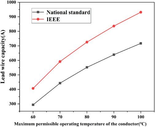
Figure 1. Relationship between bundle-conductor ampacity and maximum permissible operating temperature.

2.3 Influence of meteorological conditions on bundle-conductor ampacity

2.3.1 Effect of ambient temperature

The ampacity of overhead line is affected by the climatic condition [16]. The ambient temperature varies from 20°C to 50°C, and the result is presented in Figure 2.

Figure 2

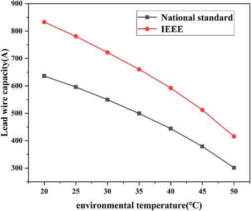
Figure 2. Relationship between bundle-conductor ampacity and ambient temperature.

As the ambient temperature increases, the corresponding bundle-conductor ampacity decreases. When the ambient temperature is lower, the conductor is able to withstand a larger current. According to the principle of heat balance, the heat dissipation of conductor mainly consists of radiation heat dissipation and convection heat dissipation. As the ambient temperature rises, the thermal conductivity of the air increases, and the heat exchange between the air and the conductor is strengthened. The temperature rise of the conductor is slightly less than the rise in ambient temperature. The temperature difference between the conductor and the surrounding air are reduced, which results in the difficulty of heat dissipation in the conductor and a decrease in the current-carrying capacity.

2.3.2 Effect of wind speed

The ambient temperature is set to 20°C, and other conditions remain unchanged. Assuming that the wind direction is perpendicular to the conductor, the wind speed changes from 0.1 m/s and gradually increases to 2 m/s, as shown in Figure 3.

Figure 3

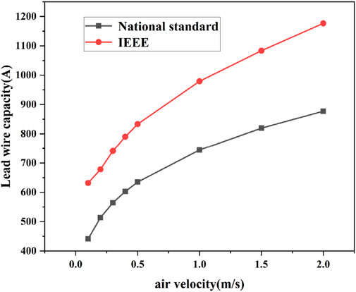
Figure 3. Relationship between bundle-conductor ampacity and wind speed.

It can be concluded that the conductor-carrying capacity increases as the wind speed rises. The convective heat dissipation power is closely related to the wind speed. The larger the wind speed, the greater the heat transfer coefficient of air layer on the wire. The convective heat dissipation power is thus greater, and the wire can withstand a larger current. Moreover, the increase range of the current-carrying capacity is relatively significant in the wind speed of 0.1 m/s to 0.5 m/s. It indicates that the current-carrying capacity of wire is sensitive to the wind speed.

2.3.3 Effect of light intensity

The maximum allowable operating temperature of the wire is set to 70°C, the ambient temperature is set to 20°C, the size of the wind speed is set to 0.5 m/s, and other conditions remain unchanged. Light intensity is changed from 500 W/m² to 1000 W/m², the curve between the maximum allowable operating temperature of wire and the light intensity is given in Figure 4.

Figure 4

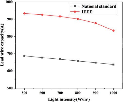
Figure 4. Relationship between bundle-conductor ampacity and sunshine intensity.

As the light intensity increases, the bundle-conductor ampacity decreases. According to the principle of heat balance analysis, light heat absorption power is proportional to the light intensity. The greater the light intensity, the more heat absorbed by the wire, and the higher the wire temperature. Hence, the current-carrying capacity is reduced. When the maximum allowable operating temperature of wire is determined, meteorological factors, including ambient temperature, solar radiation intensity and wind speed, collectively affect the actual bundle-conductor ampacity [17]. Therefore, considering real-time meteorological conditions, the bundle-conductor ampacity can be assessed more accurately by using the prediction technique [18].

3 Three-dimensional modelling of overhead bundle-conductors

Bundle-conductor, as the main carrier of UHV transmission line, is significantly affected by the coupling of electric-thermal-fluid multi-physical fields. By integrating the real geometrical parameters, dynamic material properties and meteorological condition-driven boundary settings, the electric-thermal-fluid coupling model of a four-bundle- JL/G1A-400/35 steel-core aluminum stranded wire is established.

3.1 Governing equations

3.1.1 Electromagnetic field

The conservation relationship for current can be described by Equation 11:

$\nabla ·\mathbf{J}=Q_{j,v}(11)$

The left term of Equation 10 is the scatter of the current density J, which represents the net outflow of current per unit volume. Its right side Q_j,v, is the volumetric current source, and represents the externally injected current density. Under steady-state conditions, charge accumulation is zero. Hence, the current scatter is almost determined by the external source.

The intrinsic equation for current density can be described by Equation 12:

$\mathbf{J}=\sigma \mathbf{E}+j\omega \mathbf{D}+{\mathbf{J}}_e(12)$

It defines the components of the current density:

Conduction current density (σE) is determined by conductivity σ and electric field E, corresponding to Ohm’s law.

Displacement current density (jωD) is related to the time variation of electric field, D = εE (ε is the dielectric constant).

External current density (J_e): the current density introduced by an external excitation (e.g., current source).

The relationship between electric field and electric potential can be described by Equation 13:

$\mathbf{E}=-\nabla V(13)$

3.1.2 Heat transfer field

The energy conservation equation for heat transfer in solids can be expressed by Equation 14:

$\rho C_p\mathbf{u}·\nabla T+\nabla ·\mathbf{q}=Q+Q_{ted}(14)$

where ρ is the density of the material, C_p is the constant pressure heat capacity of the material. u is the velocity field, which represents the flow rate of the fluid. T is the temperature, q is the heat flow density vector, which represents the direction and magnitude of the heat transfer. Q is the internal volumetric heat source. Q_ted is the heat due to the electromagnetic effect. The energy conservation equation for heat transfer in fluid can be expressed by Equation 15:

$\rho C_p\mathbf{u}·\nabla T+\nabla ·\mathbf{q}=Q+Q_p+Q_{vd}(15)$

where Q_p is the heat source due to pressure work and Q_vd is the viscous dissipation, i.e., the heat generated by fluid friction.

Heat conduction equation can be expressed by Equation 16:

$\mathbf{q}=-k\nabla T(16)$

where k is the thermal conductivity of the material. This equation defines the relationship between the heat flow density q and the temperature field T.

3.1.3 Fluid field

The momentum conservation equation can be defined by Equation 17:

$\rho \left(\mathbf{u}·\nabla \right)\mathbf{u}=\nabla ·\left(-p\mathbf{I}+\mathbf{K}\right)+\mathbf{F}(17)$

where p is the fluid pressure, I is the unit tensor, K is the viscous stress tensor, and F is an external volumetric force (e.g., gravity). The specific form of the viscous stress tensor K can be calculated by Equation 18:

$\mathbf{K}=\left(\mu +{\mu }_t\right)\left[\nabla \mathbf{u}+{\left(\nabla \mathbf{u}\right)}^T\right](18)$

where μ is the dynamic viscosity of the fluid and μ_t is the turbulent viscosity, which is used to describe the additional viscous effect in turbulent flow. It is defined by Equation 19:

${\mu }_t=\rho C_{\mu }\frac{k^2}{ϵ}(19)$

where ρ is the density of the fluid, k is the turbulent kinetic energy, and ϵ is the turbulent dissipation rate. C_μ is an empirical parameter and is set to 0.09.

The continuity equation is defined by Equation 20:

$\rho \nabla ·\mathbf{u}=0(20)$

For incompressible fluids, the density ρ is constant, which implies that the mass of fluid flowing into a particular tiny control body is equal to the mass of fluid flowing out of it.

Turbulent kinetic energy equation can be expressed by Equation 21:

$\rho \left(\mathbf{u}·\nabla \right)k=\nabla ·\left[\left(\mu +\frac{{\mu }_t}{{\sigma }_k}\right)\nabla k\right]+P_k-\rho ϵ(21)$

Turbulent kinetic energy k is an important parameter describing the intensity of turbulence. The left side of Equation 20 contains the convective term of turbulent kinetic energy, while its right side comprises three distinct components: the diffusion term, production term, and dissipation term of turbulent kinetic energy. σ_k is the turbulent kinetic energy Planck’s number, and is often set to be 1. The generating term of the turbulent kinetic energy P_k is computed from the velocity gradient. The turbulence viscosity is determined by Equation 22:

$P_k={\mu }_T\left[\nabla \mathbf{u}:\left(\nabla \mathbf{u}+{\left(\nabla \mathbf{u}\right)}^T\right)\right](22)$

where the double dot product () denotes the tensor reduction and merging operation.

The turbulent dissipation rate equation is determined by Equation 23:

$\rho \left(\mathbf{u}·\nabla \right)ϵ=\nabla ·\left[\left(\mu +\frac{{\mu }_T}{{\sigma }_{ϵ}}\right)\nabla ϵ\right]+C_{{ϵ}_1}\frac{ϵ}{k}{P}_k-C_{{ϵ}_2}\rho \frac{{ϵ}^2}{k}(23)$

The turbulent dissipation rate ϵ describes the rate when turbulent kinetic energy is converted to thermal energy. The equation is similar to the turbulent kinetic energy equation. σ_ϵ is the dissipation rate Platt’s number, which is generally 1.3. C_ϵ1 and C_ϵ2 are empirical constants, and they are 1.44 and 1.92 in the standard k-ε model, respectively.

3.2 Simulation study

3.2.1 Simulation model

The outer diameter of the four-bundle- JL/G1A-400/35 steel-core aluminum stranded wire is 26.8 mm, and the spacing is 450 mm. The basic parameters are given in Table 1. As shown in Figure 5, it has seven steel cores which are arranged according to the way of one inner layer and 6 outer layers. 48 aluminum wires are arranged according to the way of 10 inner layers, 16 next outer layers and 22 outermost layers.

Table 1

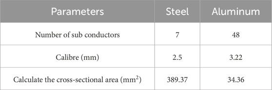
Table 1. JL/G1A-400/35 steel core aluminum stranded wire parameters.

Figure 5

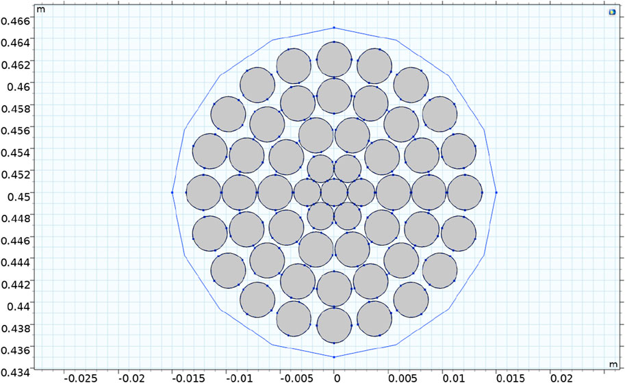
Figure 5. Cross section for JL/G1A-400/35 steel core aluminum stranded wire model sub conductor.

To conductor the electromagnetic-thermal-fluid coupling calculation of steel-core aluminum stranded wire, the material properties are defined, as listed in Table 2.

Table 2

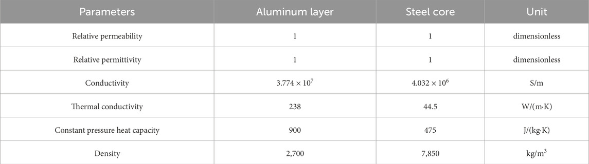
Table 2. Parameters for JL/G1A-400/35 steel core aluminum stranded wire.

3.2.2 Simulation results

To optimize computational efficiency while maintaining simulation accuracy, the model adopts the following geometric parameters: each of the bundle-conductor has a length of 0.1 m, enclosed within a cylindrical air domain with a radius of 0.5 m and height of 0.1 m, as shown in Figure 6. The computational domain is discretized using grid generation techniques, which transform the continuous geometric space into discrete computational cells. This discretization enables numerical analysis of complex geometries and physical field distributions.

Figure 6

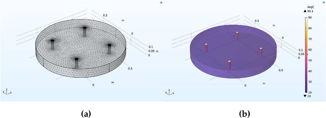
Figure 6. Developed Model in COMSOL: (a) Four bundle- JL/G1A-400/35 conductor model grid section schematic diagram. (b) Temperature distribution of the four-bundle- JL/G1A-400/35 model.

4 Prediction model

The meteorological factors, including ambient temperature, wind speed and light intensity, determine the size of bundle-conductor ampacity. The key to obtain the predicted value of the conductor ampacity is optimally leveraging the respective advantages of existing algorithms. It serves as the prerequisite for coupling higher-performance model combinations.

4.1 Transformer coding layer

The Transformer encoder layer enhances the Transformer-LSTM network by generating attention-weighted data. The processed data can provide more features in the prediction of carrier traffic. Through dot-product operations, the Transformer coding layer generate attention to the data, while multiple identical encoder layers operating in parallel enable efficient data processing and prediction. The structures of Transformer coding layer are the multi-head attention mechanism and the feed-forward layer. Layer normalization operation is added after each multi-head attention mechanism and feed-forward layer. The data processed by layer normalization can reduce problems, such as gradient explosion and improve the stability of the network. To retain the original data characteristics during the processing, the encoder architecture includes two linear summation layers, which improve the model feature learning. Transformer coding layer structure is presented in Figure 7.

Figure 7

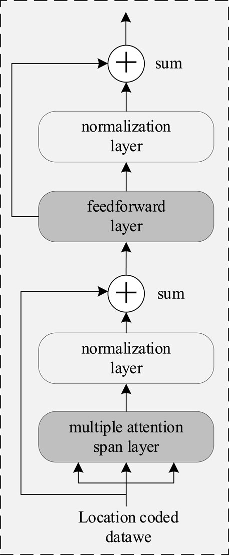
Figure 7. Transformer coding layer structure.

The core part of the coding layer is the multi-head attention mechanism. It is the key part of the Transformer-LSTM model to realize accurate prediction. The multi-head attention strength mechanism consists of multiple heads with self-attention. The self-attention can be described as a process solved by a query vector and a set of key-value vector matrices. The model simultaneously computes the attention function on a set of query vectors and packs them into a matrix Q, and packs the key-value vectors and the value vectors into matrices K and V. The output of the query vectors is determined by the hidden vectors encoded in the previous layer, and the matrices K and V are assigned the same value as Q in the self-attention. The output is the weight-weighted value, which is derived from the compatibility operation between the query vector and the key vector. f = {f_i}^t_i=1 is the input of the multi-head self-attention module. The key vectors, weight vectors and query vectors are calculated by Equation 24:

${\mathit{K}}_j=f{\mathit{W}}_j^k(24)$

${\mathit{V}}_j=f{\mathit{W}}_j^v(25)$

${\mathit{Q}}_j=f{\mathit{W}}_j^q(26)$

where $W_j^k,W_j^k,W_j^k\in R^{d\times d_k}$ is the trainable projection matrix. Using the derived results, the scaled dot calculation can be expressed by Equation 27:

$\text{Attention}{\left(Q,K,V\right)}_j=\text{softmax}\left(\frac{Q_j{K}_j^{\mathrm{T}}}{\sqrt{d_k}}\right)V_j(27)$

In order to focus on the information from various representation subspaces at different locations, further optimization is required by using H parallel attention computations. In the case of $W^A\in R^{H{d}_k\times d}$, the process of the multi-head attention mechanism is calculated by Equation 28:

$\text{MultiHead}\left(Q,K,V\right)=\text{Concat}\left({\left\{hea{d}_j\right\}}_{j=1}^H\right)W^A(28)$

The functionality of encoder layer is processed by a feed-forward network. This network implements two sequential linear transformations with a ReLU activation function between them, applied uniformly across all temporal positions. The linear transformation formula can be expressed by Equation 29:

$y=W^{\mathrm{T}}x+b(29)$

4.2 LSTM decoding layer

The improvement of Transformer-LSTM network model is architectural reconstruction of the decoding layer of the original Transformer. When the original Transformer decoding layer is applied in the field of regression computation, the decoding layer is replaced by a linear layer. Hence, the prediction model produces a large bias in the prediction of short data sets. To enhance the predictive performance, a redesigned LSTM-based decoding layer is proposed, which consists of a linear rectification layer, an LSTM processing layer and a fully connected output layer. The core part is LSTM operation layer and LSTM decoding layer, as shown in Figure 8. The linear rectifier processes the output of Transformer encoding layer, and transform the data into a format compatible with the LSTM hidden layer, thereby facilitating effective input representation.

Figure 8

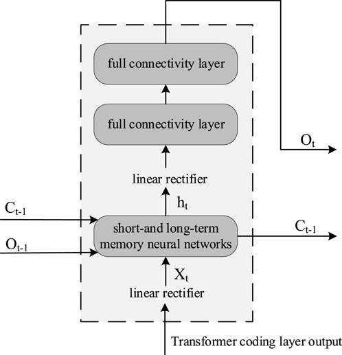
Figure 8. LSTM decoding layer structure.

The LSTM operation layer consists of input gates, forgetting gates, output gates and cell states. The structure of LSTM network is given in Figure 9. The LSTM module processes sequential data by integrating three input sources: i) the encoded data from the Transformer layer; ii) the hidden data h_t from the previous time step; iii) the cell state output C_t. These inputs are sequentially processed through the gating mechanism to enable effective temporal modeling.

Figure 9

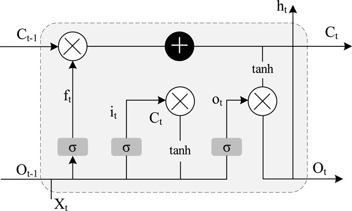
Figure 9. LSTM network structure.

The data is calculated in the input gate according to Equation 30:

$i_t=\sigma \left(W_i\left[h_{t-1},x_t\right]+b_i\right)(30)$

The data is calculated in the forgetting gate according to Equations 31, 32:

$f_t=\sigma \left(W_f\left[h_{t-1},x_t\right]+b_f\right)(31)$

${\widehat{C}}_t=\tanh \left(W_C\left[h_{t-1},x_t\right]+b_C\right)(32)$

The data is calculated in the output gate according to Equation 33:

$o_t=\sigma \left(W_o\left[h_{t-1},x_t\right]+b_o\right)(33)$

The gated outputs are subsequently distributed to two distinct memory modules, where long-term and short-term dependencies are selected to be processed by specialized pathways, as follows:

The long memory is described by Equation 34:

$C_t=f_t*C_{t-1}+i_t*{\widehat{C}}_t(34)$

The short memory is described by Equation 35:

$O_t=o_t*\tanh \left(C_t\right)(35)$

Before the output of the improved LSTM decoder, the two additional fully connected layers are applied to enhance the network robustness and increase the output reliability.

4.3 Overall structure of Transformer-LSTM network

The mechanism of the data processing in Transformer-LSTM network can be categorized into two distinct phases: intra-cell processing and inter-cell processing. To realize the load capacity prediction, the data is transferred in two ways. The intra-cell processing performs the parallel computation of feature transformations, while the inter-cell processing facilitates sequential information flow across temporal or spatial dimensions. The data within the cell follows the designated pathway (Route ①), as illustrated in Figures 10, 11. Each input is position coded as well as Transformer coded. Therefore, the encoded data retains more feature hierarchies to ensure less signal attenuation during the load prediction process.

Figure 10

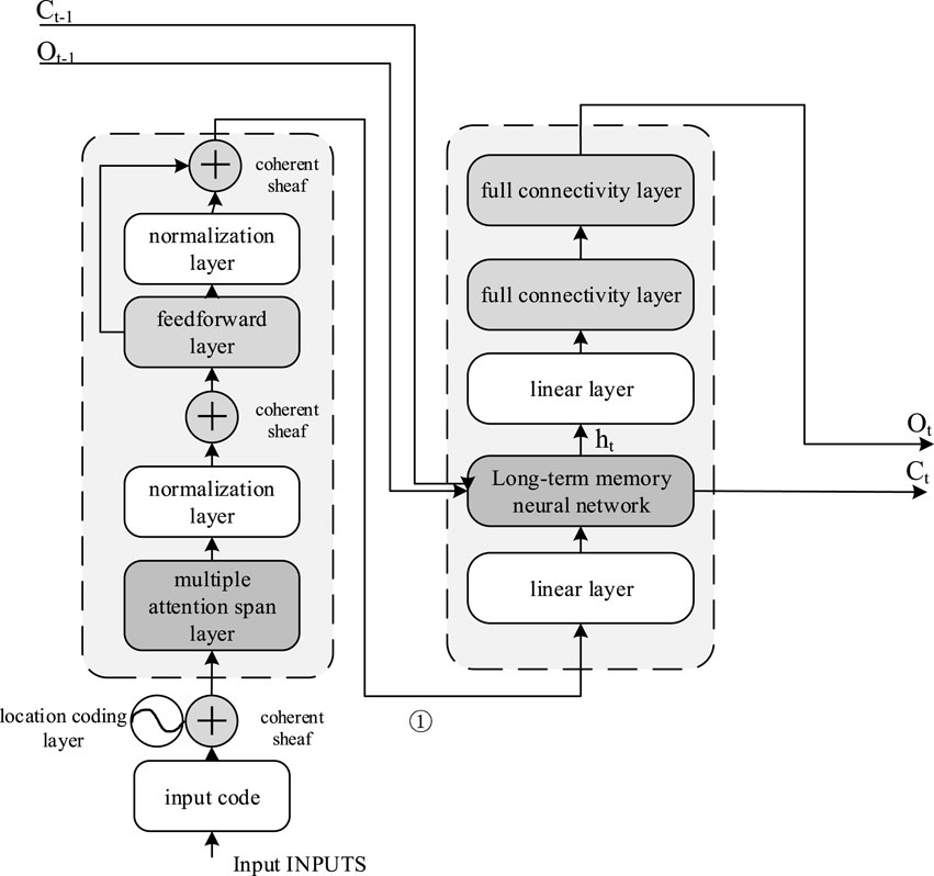
Figure 10. Transformer-LSTM intra-cell network structure.

Figure 11

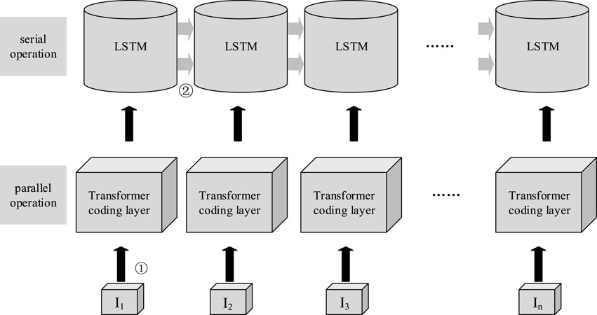
Figure 11. Transformer-LSTM data transfer process.

The transfer model of data is given in Figure 11. The out-of-cell data processing is implemented through the LSTM-based decoding layer, which achieves complete preservation of temporal dependencies by its gated memory, as illustrated in ② of Figure 11. The architecture enables effective sequential pattern learning, thereby improving the prediction performance of the network.

5 Discussion

5.1 Prediction process

The proposed Transformer-LSTM model implements load capacity prediction through the following technical route: 1) a dataset is constructed by integrating meteorological parameters by using COMSOL. 2) Normalize the feature dataset. 3) Build Transformer-LSTM model. 4) The dataset is partitioned into training and validation subsets, with the former utilized for model optimization and the latter employed for performance evaluation. 5) A joint training-prediction dataset is constructed to enable comprehensive quantitative evaluation of model performance. The framework is presented in Figure 12.

Figure 12

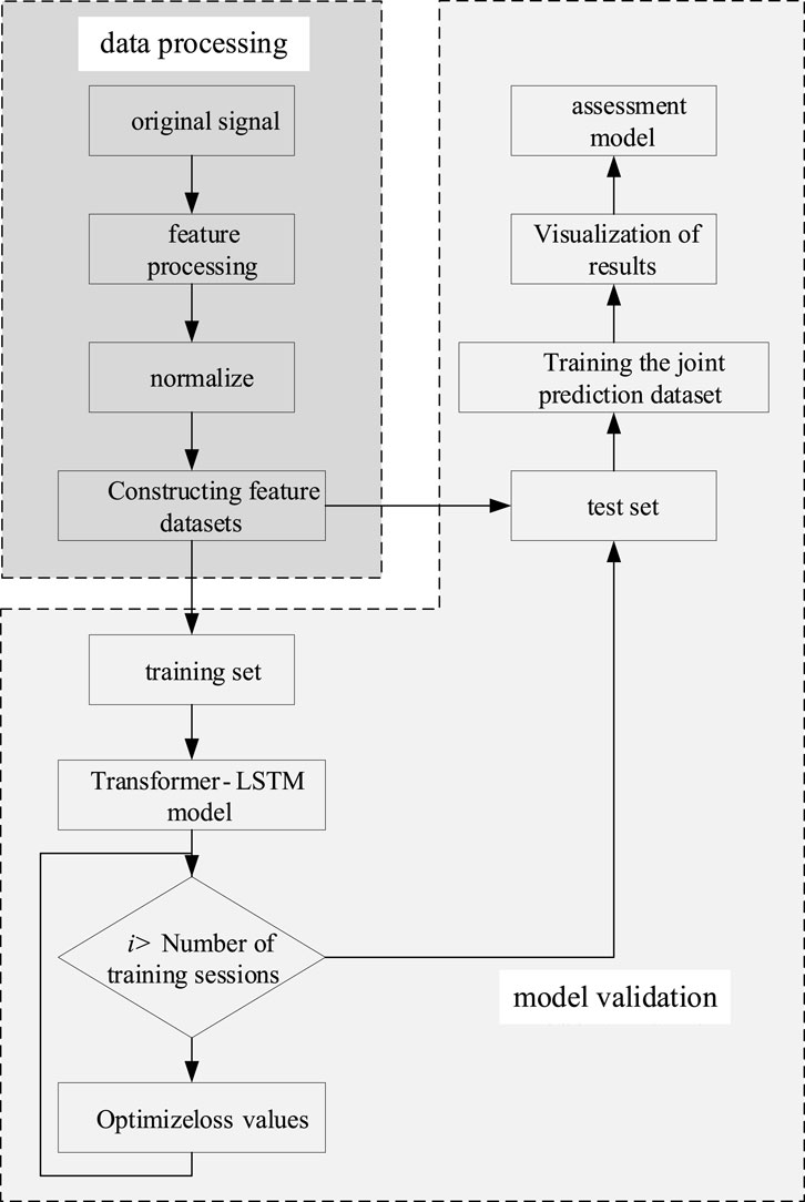
Figure 12. Flowchart for prediction.

A JL/G1A-400/35 steel-core aluminum strand wire is established, and the spacing between sub-conductor is 0.45 m. The wind speed is set to 0.5 m/s, 1.0 m/s, 1.5 m/s and 2.0 m/s. The light intensity is 100 W/m², 500 W/m² and 1,000 W/m². The ambient temperature is set to 0 10°C, 20°C, 30°C and 40°C. A total of 4 × 3 × 5 = 60 combinations are selected. The calculations are conducted for each combination to determine the current when the conductor temperature is the maximum allowable operating temperature (i.e., 70°C). 60 samples are obtained, which are divided into 42 training subsets and 18 validation subsets.

5.2 Model parameterization and evaluation indicators

5.2.1 Model parameterization

The Transformer-LSTM model is trained and tested with the following configurations: for hardware level, CPU is AMD Ryzen 55,600 and GPU is NVIDIA GeForce RTX 3060 TI (8 GB). For the software level, it is built based on Windows 11 64-bit operating system. The programming language is Python 3.8, and the deep learning framework is PyTorch 1.8. It is chosen as the deep learning framework, while the GPU is accelerated by CUDA 11.1. The details for training model are listed in Table 3.

Table 3

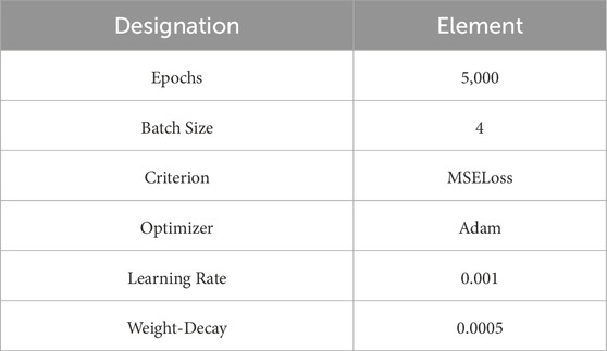
Table 3. Model hyperparameter settings.

5.2.2 Evaluation indicators

Evaluation indexes are important for model prediction accuracy. In this paper, the mean square error (MSE) and mean absolute error (MAE) are selected as the evaluation indexes of prediction results. They are defined by Equations 36, 37:

$MSE=\frac{1}{N}{\displaystyle \sum _{i=1}^N}{\left(y_i-y_p\right)}^2(36)$

$MAE=\frac{1}{N}{\displaystyle \sum _{i=1}^N}\left|y_i-y_p\right|(37)$

where y_i is the true value, y_p is the value predicted by model, and N is the number of samples.

5.3 Prediction results

5.3.1 Training process

During the training process of Transformer-LSTM model, the regression curves demonstrate excellent fitting performance on both the training and validation subsets, indicating strong learning capability and generalization capacity of the proposed model, as illustrated in Figure 13. The regression curves on the training subset can closely fit the actual data points. It is confirmed that the model is successfully capture the complex nonlinear relationships and long-term dependency features in data through the synergistic combination of Transformer self-attention and LSTM modeling capability. The regression curves on the validation subset also show high prediction accuracy with small deviation from the actual data, and the model is not over fitted.

Figure 13

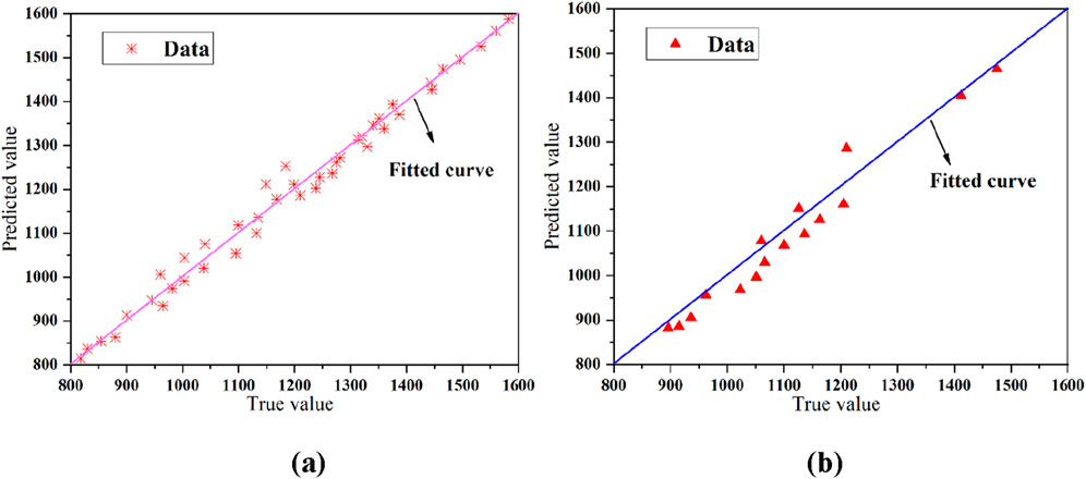
Figure 13. Regression curves: (a) Training set (b) Test set.

5.3.2 Discussion

The prediction results are given in Table 4. It demonstrates that the proposed model can accurately capture the complex correlation between the carrier volume and meteorological factors. For the dynamic combination of wind speed (0.5–2.0 m/s), light intensity (100–1000 W/m²) and ambient temperature (0°C–40°C), the maximum relative error between the predicted value and the actual value is only 3.76%. It is at a high degree of consistency for most conditions. Notably, the proposed model demonstrates robust predictive performance under extreme meteorological conditions, maintaining consistently high accuracy (e.g., achieving merely 0.56% prediction error for the [21,000 10] configuration). This performance persists even under thermally stressful (30°C–40°C ambient temperature) and high irradiance (1000 W/m² solar loading) conditions. These results validate that the model can capture nonlinear interactions between coupled physical fields in the power transmission scenario through its advanced feature representation mechanism. The Transformer-LSTM architecture enables accurate prediction of bundle-conductor ampacity. It can offer highly reliable decision support for thermal balance analysis and real-time transmission capacity regulation under dynamic weather conditions.

Table 4

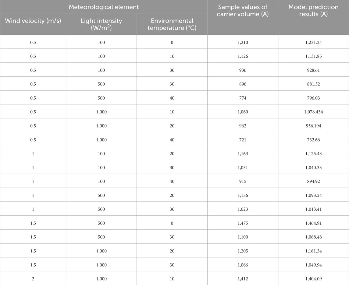
Table 4. Prediction results of model on test set.

In order to verify the superiority of the proposed model, it is compared with three representative benchmark algorithms, such as Support Vector Regression (SVR), Random Forest (RF), and Bidirectional Long Short-Term Memory Network (BiLSTM). The results are given in Table 5. The prediction errors of the proposed model are all lower than those of SVR, RF and BiLSTM models. Compared with BiLSTM model, the MSE and MAE of the proposed model are decreased by 74.55% and 7.35%, respectively. The effectiveness and significant solution advantages of the Transformer-LSTM model are validated.

Table 5

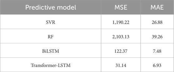
Table 5. Prediction results for bundle-conductor ampacity.

Moreover, several sets of typical meteorological factors, including wind speed, light intensity and ambient temperature, are considered. The load capacity predicted by the Transformer-LSTM model is compared with that from conventional methods, as presented in Table 6.

Table 6

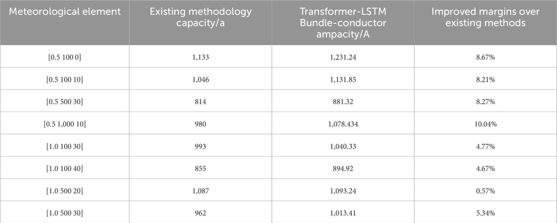
Table 6. Comparison of Transformer-LSTM with existing methods.

It can be concluded that the ampacity calculated by the Transformer-LSTM model is larger than that of the existing method. The conventional calculation method of bundle-conductor ampacity is conservative, whereas the Transformer-LSTM model enhances the capacity margin by up to 10%. More effective utilization of transmission potential of overhead lines is realized by Transformer-LSTM model. When implemented in power systems, the proposed model enables dynamic adjustment of overhead transmission line capacity during peak demand periods based on its predictive outputs.

6 Conclusion

A hybrid modeling method, which combines multi-physics field simulation with neural network deep learning, is proposed to address the overhead bundle-conductor load capacity prediction problem. The conclusions are summarized as follows.

• A 3D electro-thermal-fluid coupled model is developed to analyze the conductor temperature rise under complex meteorological conditions. It can provide a physics-based foundation for bundle-conductor ampacity assessment.

• The Transformer-LSTM algorithm is designed to establish a high-precision nonlinear mapping between meteorological parameters and bundle-conductor ampacity, improving prediction robustness.

• The experimental results demonstrate that the proposed model outperforms traditional prediction models in accuracy, confirming its practical applicability in load capacity prediction.

Data availability statement

The original contributions presented in the study are included in the article/supplementary material, further inquiries can be directed to the corresponding author.

Author contributions

SB: Investigation, Software, Validation, Writing – original draft. HB: Resources, Software, Writing – review and editing. MJ: Formal Analysis, Validation, Writing – review and editing. YR: Data curation, Writing – review and editing. YS: Conceptualization, Writing – review and editing. CY: Formal Analysis, Writing – review and editing.

Funding

The author(s) declare that financial support was received for the research and/or publication of this article.

Conflict of interest

Authors SB, HB, MJ, YR, YS, and CY were employed by China Energy Engineering Group Anhui Electric Power Design Institute Co., LTD.

The authors declare that this study received funding from China Energy Engineering Group Anhui Electric Power Design Institute Co., Ltd. under Grant Numbers KBY2022016. The funder had the following involvement in the study: study design, data collection and analysis, decision to publish, and preparation of the manuscript.

Generative AI statement

The author(s) declare that no Generative AI was used in the creation of this manuscript.

Publisher’s note

All claims expressed in this article are solely those of the authors and do not necessarily represent those of their affiliated organizations, or those of the publisher, the editors and the reviewers. Any product that may be evaluated in this article, or claim that may be made by its manufacturer, is not guaranteed or endorsed by the publisher.

References

1. Ying X, Qige Y, Fengming Q, Kai L, Ruipeng L, Mulang W. Key circuit current-carrying capacity verification and its improvement via 3D holographic capacity expansion technique. In: 2024 9th asia conference on power and electrical engineering. Shanghai, China: ACPEE (2024). p. 1786–91. doi:10.1109/ACPEE60788.2024.10532427

CrossRef Full Text | Google Scholar

2. Han P, Li P, Xie X, Zhang J. Coordinated optimization of power rating and capacity of battery storage energy system with large-scale renewable energy. In: 2022 IEEE 6th conference on energy internet and energy system integration (EI2). China: Chengdu (2022). p. 189–93. doi:10.1109/EI256261.2022.10116240

CrossRef Full Text | Google Scholar

3. Michiorri A, Nguyen H-M, Alessandrini S, Bremnes JB, Dierer S, Ferrero E, et al. Forecasting for dynamic line rating. Renew Sustain Energ Rev (2015) 52:1713–30. ISSN 1364-0321. doi:10.1016/j.rser.2015.07.134

CrossRef Full Text | Google Scholar

4. Zheng Z, Chen YZ, Zhong X, Fan Q, Zhang J, Wu R, et al. Cumulative effect of reignition overvoltage caused by vacuum circuit breaker on shunt reactor insulation in offshore wind farm. IEEE Trans Power Deliv (2025) 40(2):1158–68. doi:10.1109/TPWRD.2025.3542392

CrossRef Full Text | Google Scholar

5. Wan H, Mccalley JD, Vittal V. Increasing thermal rating by risk analysis. IEEE Trans Power Syst (1999) 14(3):815–28. doi:10.1109/59.780891

CrossRef Full Text | Google Scholar

6. Cheng Y, Liu P, Zhang Z, Dai Y. Real-time dynamic line rating of transmission lines using live simulation model and tabu search. IEEE Trans Power Deliv (2021) 36(3):1785–94. doi:10.1109/tpwrd.2020.3014911

CrossRef Full Text | Google Scholar

7. Foss SD, Maraio RA. Dynamic line rating in the operating environment. IEEE Trans Power Deliv (1990) 5(2):1095–105. doi:10.1109/61.53127

CrossRef Full Text | Google Scholar

8. Douglass D, Chisholm W, Davidson G, Grant I, Lindsey K, Lancaster M, et al. Real-time overhead transmission-line monitoring for dynamic rating. IEEE Trans Power Deliv (2016) 31(3):921–7. doi:10.1109/TPWRD.2014.2383915

CrossRef Full Text | Google Scholar

9. Zhan J, Liu W, Chung CY. Stochastic transmission expansion planning considering uncertain dynamic thermal rating of overhead lines. IEEE Trans Power Syst (2019) 34(1):432–43. doi:10.1109/TPWRS.2018.2857698

CrossRef Full Text | Google Scholar

10. Aznarte JL, Siebert N. Dynamic line rating using numerical weather predictions and machine learning: a case study. IEEE Trans Power Deliv (2017) 32(1):335–43. doi:10.1109/tpwrd.2016.2543818

CrossRef Full Text | Google Scholar

11. Romain D, George K, Andrea M. Overhead lines Dynamic Line rating based on probabilistic day-ahead forecasting and risk assessment. Int J Electr Power and Energ Syst 110(2019):565–78. ISSN 0142-0615. doi:10.1016/j.ijepes.2019.03.043

CrossRef Full Text | Google Scholar

12. Moradzadeh A, Mohammadpourfard M, Genc I, Şeker ŞS, Mohammadi-Ivatloo B. Deep learning-based cyber resilient dynamic line rating forecasting. Int J Electr Power and Energ Syst (2022) 142:108257. doi:10.1016/j.ijepes.2022.108257

CrossRef Full Text | Google Scholar

13. IEEE. IEEE standard for calculating the current-temperature relationship of bare overhead conductors. IEEE Std (2013) 738–2012. doi:10.1109/IEEESTD.2013.6692858

CrossRef Full Text | Google Scholar

14. Kacejko P, Pijarski P. Dynamic fitting of generation level to thermal capacity of overhead lines. Przeglad Elektrotechniczny (2008) 84:80–3.

Google Scholar

15. Beňa Ľ, Gáll V, Kanálik M, Kolcun M, Margitová A, Mészáros A, et al. Calculation of the overhead transmission line conductor temperature in real operating conditions. Electr Eng prepublish (2020) 103:769–80. doi:10.1007/s00202-020-01107-2

CrossRef Full Text | Google Scholar

16. Zeńczak M. Approximate relationships for calculation of current-carrying capacity of overhead power transmission lines in different weather conditions. 2017 Prog Appl Electr Eng (Paee) Koscielisko, Poland (2017) 1–5. doi:10.1109/PAEE.2017.8008996

CrossRef Full Text | Google Scholar

17. Zhang G, Li S, Dai J, Zhao L, Liu Y, Wei L, et al. Probability prediction of transient current-carrying capacity of the overhead conductor with the consideration of the correlation of conductor temperature and meteorological elements. In: 2023 9th international conference on electrical engineering, control and robotics (EECR). China: Wuhan (2023). p. 134–8. doi:10.1109/EECR56827.2023.10149913

CrossRef Full Text | Google Scholar

18. Hu J, Xiong X, Wang J. Current tolerance capability calculation model of transmission lines and its application in overload protection. Electric Power Components Syst (2019) 46:1509–21. doi:10.1080/15325008.2018.1511005

CrossRef Full Text | Google Scholar