Numerical solutions of the nonlinear Fisher’s equation using a one-level meshless method

This study introduces a relatively new numerical technique for solving one-dimensional Fisher’s equation. The proposed numerical technique is a simple direct meshless method, which is based on the collocation scheme. To circumvent the traditional two-level numerical procedure, the space-time radial basis function is considered. Under such circumstances, the time-dependent one-dimensional nonlinear Fisher’s equation can be solved by a one-level numerical procedure. Several numerical results are investigated to show advantages of the proposed meshless method.

1 Introduction

The application areas of nonlinear fisher’s equation include biology [1], ecology [2] cancer research [3], chemistry [4], etc. It continues to serve the spatiotemporal dynamics modeling of complex systems, and in the future, it will deeply intersect with cutting-edge fields such as quantum computing and synthetic biology. As a classic reaction-diffusion model, the nonlinear fisher’s equation has the following form

$\frac{\mathrm{\partial }u}{\mathrm{\partial }t}=\alpha \frac{{\mathrm{\partial }}^{2}u}{\mathrm{\partial }{x}^2}+\gamma u\left(1-u\right),a<x<b,t>0.(1)$

Here, $\alpha$ denotes the constant diffusion coefficient or diffusion factor and $\gamma$ is the reaction factor which can denote growth rate or birth rate.

Numerical simulation of Fisher’s equation has made significant progress driven by computational power, algorithm innovation, and interdisciplinary demands [5]. Traditional methods include the finite difference method [6], the finite element method [7], and coupled numerical methods based on traditional methods [8–10]. By using generalized Hermite interpolation, a fully discrete pseudospectral scheme is presented for Fisher’s equation [11]. Geeta and Varun [12] investigated trigonometric B-spline collocation method to simulate the 1-D Fisher’s equation. A hybrid numerical method [13], which is composed by cubic trigonometric B-spline base functions and differential quadrature method, is proposed for the numerical solution of Fisher’s reaction-diffusion equation. Based on the finite difference method and wavelet Galerkin method, Haifa [14] proposed an algorithm to simulate the Fisher’s equation. The Haar wavelet method is applied to obtain the approximate solution for the Fisher’s equations by Sakina et al. [15]. Based on Barycentric Rational interpolation, Mittal and Rohila [16] proposed a numerical approach to simulate the Burgers’ and Fisher’s equations.

Since the radial-basis-function-based collocation methods are truly meshless numerical methods, they are widely used in solving partial differential equations and analyzing complex engineering problems. The effectiveness of the BKM is investigated for solving Helmholtz-type problems under various conditions through a series of novel numerical experiments [17]. Based on the method of fundamental solutions, a high-accuracy and efficient method is provided for addressing antiplane piezoelectricity problems with multiple inclusions [18]. A new meshfree method is proposed for heat transfer problems in porous material energy storage battery [19].

Some investigations have been performed by using radial-basis-function-based methods to simulate Fisher’s equation. Based on the global radial basis function method, Zhang et al. [20] proposed a two-level radial basis function-finite difference method for solving nonlinear Fisher’s equation. A novel meshless local collocation method is proposed for the numerical solution of the 3-D extended Fisher-Kolmogorov equation [21]. In combination with the pseudo-spectral method, Geeta et al. [22] used the radial basis function to get the numerical solution of Fisher’s equation. Along with the radial basis functions, particle swarm optimisation algorithm is used to obtain the numerical solutions of the Fisher’s equation [23].

As mentioned in the previous-analysis, there are some investigations related to the meshless method for Fisher’s equation. However, these numerical methods are two-level numerical methods. The meshless method should be accompanied with the other numerical methods to deal with time-dependent term in the governing equation. To seek for an alternative way, we propose a one-level meshless method for Fisher’s equation. By using a space-time formulation, the time-dependent term can be treated as space-dependent term. The initial and boundary conditions for Fisher’s equation are given as

$\left\{\begin{array}{l}u\left(x,0\right)=u_0\left(x\right),x\in \left\{a,b\right\},\\ u\left(x,t\right)=\overline{u}\left(x,t\right),t>0.\end{array}\right.(2)$

Here, $u_0\left(x\right)$ and $\overline{u}\left(x,t\right)$ are prescribed smooth functions.

The rest of this paper is organized as follows. Section 2 provides a brief description of the one-level meshless method. Numerical examples are provided in Section 3 and some concluding remarks are given in Section 4.

2 The one-level meshless methods

As is known to all, the time-dependent problems Equations 1, 2 are always solved by using two-level numerical methods. The finite difference scheme or integral transform method should be employed to deal with the time-dependent term, and the resulting elliptic-type problems are solved by the other numerical methods. There are two aspects in the accumulation of errors of two-level methods, i.e., the finite difference step and the numerical method step.

To find an alternative to the two-level method, a one-level direct meshless method is proposed in this section. The one-level direct meshless method is based on space-time radial basis functions (RBFs). Under such one-level meshless method, there’s only one aspect in the accumulation of errors.

2.1 The space-time RBFs

RBFs are a type of scalar function based on distance measurement, whose core characteristic is that the function value only depends on the distance from the two points. The advantages of RBFs include local response characteristics, efficient processing of sparse or high-dimensional data, simple mathematical form, easy-to-implement, and parallel computing.

For 2D steady-state problems, the commonly-used RBFs include three types, the detailed formula is shown in Equation 3

$\phi \left(r\right)=\left\{\begin{array}{l}\sqrt{1+{\left(\epsilon r\right)}^2},\text{Multiquadric},\\ e^{-{\left(\epsilon r\right)}^2},\text{Gaussian},\\ r^2\log r,\text{Thin\hspace{0.5em}Plate\hspace{0.5em}Spline}.\end{array}\right.(3)$

Here, $r=‖X_i-X_j‖$ is the Euclidean distance between two points $X_i=\left(x_i,y_i\right)$ and $X_j=\left(x_j,y_j\right)$, $\epsilon$ is the RBF shape parameter.

Since there is only one space variable in Fisher’s Equation 1, we consider the time variable “equally” as a new space variable. More specifically, the Fisher’s equation is considered as a “equally” steady-state equation. The corresponding space-time RBFs has the form

$\varphi \left(\overline{r}\right)=\left\{\begin{array}{l}\sqrt{1+{\left(\epsilon \overline{r}\right)}^2},\text{Multiquadric},\\ e^{-{\left(\epsilon \overline{r}\right)}^2},\text{Gaussian},\\ {\overline{r}}^2\log \overline{r},\text{Thin\hspace{0.5em}Plate\hspace{0.5em}Spline}.\end{array}\right.(4)$

Here, $\overline{r}=\sqrt{{\left(x_i-x_j\right)}^2+{\left(t_i-t_j\right)}^2}$ is the Euclidean distance between two space-time points ${\overline{X}}_i=\left(x_i,t_i\right)$ and ${\overline{X}}_j=\left(x_j,t_j\right)$.

2.2 Implementation of the one-level meshless method

Before implementation of the one-level meshless method, collocation points should be provided. More specifically, the space variable interval $\left[a,b\right]$ is divided into small segments $a=x_0<x_1<...<x_n=b$ and the time variable interval $\left[0,T\right]$ is divided into segments $0=t_0<t_1<...<t_n=T$. The interval division is usually under uniform scheme, but it is also workable for un-uniform scheme.

According to the basic theory of collocation methods, the approximate solution of the function $u\left(x,t\right)$ at an arbitrary point $\overline{X}=\left(x,t\right)$ in Fisher’s equation has the form

$\overline{u}\left(·\right)\approx {\displaystyle \sum _{j=1}^N}{\lambda }_j{\varphi }_j\left(·\right)(5)$

with ${\left\{{\lambda }_j\right\}}_{j=1}^N$ the unknown coefficients and ${\varphi }_j\left(·\right)=\sqrt{1+{\left(\epsilon {\overline{r}}_j\right)}^2}=\sqrt{1+{\epsilon }^2{\left(x-x_j\right)}^2+{\epsilon }^2{\left(t-t_j\right)}^2}$, where $j$ is the index of collocation points and $N$ is the total collocation point number.

To illustrate the one-level meshless method, we substitute Equation 6 into Equations 1, 2 at space-time points ${\left\{{\overline{X}}_k=\left(x_k,t_k\right)\right\}}_{k=1}^{n\times n}$. Then, one can obtain the following equations

${\displaystyle \sum _{j=1}^N}{\lambda }_j\mathcal{L}{\varphi }_j\left({\overline{X}}_k,{\overline{X}}_j\right)=0,k=1,...,{\left(n-2\right)}^2,(6)$

$\left\{\begin{array}{l}{\displaystyle \sum _{j=1}^N}{\lambda }_j{\varphi }_j\left({\overline{X}}_k,{\overline{X}}_j\right)=u_0\left({\overline{X}}_k\right),\\ {\displaystyle \sum _{j=1}^N}{\lambda }_j{\varphi }_j\left({\overline{X}}_k,{\overline{X}}_j\right)=\overline{u}\left({\overline{X}}_k\right),\end{array}\right.k={\left(n-2\right)}^2+1,...,n^2.(7)$

Here, the operator is shown in the following Equation 8

$\mathcal{L}{\varphi }_j=\alpha \frac{{\mathrm{\partial }}^2{\varphi }_j}{\mathrm{\partial }{x}^2}-\frac{\mathrm{\partial }{\varphi }_j}{\mathrm{\partial }t}+\gamma {\varphi }_j\left(1-{\varphi }_j\right).(8)$

For multiquadric RBF ${\varphi }_j\left(r\right)=\sqrt{1+{\left(\epsilon {\overline{r}}_j\right)}^2}=$ $\sqrt{1+{\epsilon }^2{\left(x-x_j\right)}^2+{\epsilon }^2{\left(t-t_j\right)}^2}$, we have the corresponding derivatives in Equations 9–11

$\frac{\mathrm{\partial }{\varphi }_j}{\mathrm{\partial }x}={\epsilon }^2\left(x-x_j\right){\left(1+{\epsilon }^2{\overline{r}}_j^2\right)}^{-\frac{1}{2}},(9)$

$\frac{{\mathrm{\partial }}^2{\varphi }_j}{\mathrm{\partial }{x}^2}={\epsilon }^2{\left(1+{\epsilon }^2{\overline{r}}_j^2\right)}^{-\frac{1}{2}}\left[1-{\epsilon }^2{\left(x-x_j\right)}^2/\left(1+{\epsilon }^2{\overline{r}}_j^2\right)\right],(10)$

$\frac{\mathrm{\partial }{\varphi }_j}{\mathrm{\partial }t}={\epsilon }^2\left(t-t_j\right){\left(1+{\epsilon }^2{\overline{r}}_j^2\right)}^{-\frac{1}{2}}.(11)$

In order to obtain a square interpolation matrix, we consider $N=n\times n$. Equations 6, 7 has the matrix form as shown in Equation 12

$\mathbf{A}\lambda =\mathbf{f},(12)$

where $\mathbf{A}=\left[{\varphi }_{kj}\right]$ is $N\times N$ interpolation matrix, $\lambda$ and $\mathbf{f}$ are $N\times 1$ vectors.

Equation 9 can be directly solved to get the unknowns $\lambda$. Then the approximation solution of the unknown function in the Fisher’s equation can be solved by using Equation 5.

3 Numerical simulations

In the following numerical examples, the multiquadrics RBF in Equation 4 is used to illustrate the numerical results. We use the $L_2-\text{error}$ to show the accuracy of the proposed method. The $L_2-\text{error}$ of the proposed method is also compared with the results in previous literatures. The optimal choice of RBF parameter has been investigated in many literatures [24, 25]. This is beyond the scope of our current research, we use the simple prior-tested selection of the shape parameter in all numerical results [26, 27]. Due to the limitation of the paper type, the initial condition plots are provided in the appendix.

3.1 Example 1

For the constant diffusion coefficient $\alpha =1$ and the reaction factor $\gamma =6$, the fisher’s equation has the form in Equation 13

$u_t=u_{xx}+6u\left(1-u\right),-1<x<1,0<t<T.(13)$

The corresponding exact solution is

$u\left(x,t\right)=\frac{1}{{\left(1+e^{x-5t}\right)}^2}.(14)$

The corresponding initial condition and boundary condition can be deduced from Equation 14.

At time $t=1$, the variation of shape parameter versus the $L_2-\text{error}$ is presented in Figure 1 for fixed collocation point number $N=117$. It can be seen that the quasi-optimal $L_2-\text{error}$ is $6.8893\times {10}^{-8}$ for shape parameter $\epsilon =1.45$. This is more accurate than the most accurate numerical result $4.33\times {10}^{-5}$ in [14]. For shape parameter $\epsilon =1.45$, Figure 2 is plotted to show that the numerical solution is highly consistent with the analytical solution.

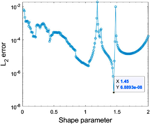
Figure 1

Figure 1. $L_2-\text{error}$ curve versus shape parameter.

Figure 2

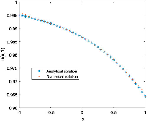
Figure 2. Numerical solution and analytical solution at time $t=1$.

3.2 Example 2

Here, we consider the following Fisher’s equation as shown in Equation 15

$u_t=u_{xx}+u\left(1-u^6\right),-1<x<1,0<t<T(15)$

The corresponding exact solution is shown in Equation 16

$u\left(x,t\right)={}^3\sqrt{\frac{1}{2}\tanh \left(-\frac{3x}{4}+\frac{15t}{8}\right)+\frac{1}{2}}.(16)$

The quasi-optimal choice of shape parameter is the same as Example 4.1. For shape parameter $\epsilon =0.44$, the $L_2-\text{error}$ is $2.8366\times {10}^{-10}$ at time $t=1$, which is also far more accurate than the most accurate result $1.27\times {10}^{-5}$ in [14]. Figure 3 is plotted to show that the numerical solution is highly consistent with the analytical solution at three different times $t=0.1,t=0.5,t=1$.

Figure 3

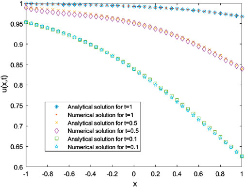
Figure 3. Numerical solution and analytical solution at times $t=0.1,t=0.5,t=1$.

3.3 Example 3

In this example, we consider the following Fisher’s equation as shown in Equation 17

$u_t=u_{xx}+u\left(1-u^2\right),-1<x<1,0<t<T.(17)$

The corresponding analytical solution is shown in Equation 18

$u\left(x,t\right)=-\frac{1}{2}\tanh \left(\frac{\sqrt{2}}{4}\left(x-\frac{\sqrt{18}t}{2}\right)\right)+\frac{1}{2}.(18)$

At time $t=1$, the quasi-optimal choice of shape parameter is $\epsilon =0.49$ with the corresponding $L_2-\text{error}$ $2.3819\times {10}^{-8}$. It is also more accurate than the most accurate result $6.00\times {10}^{-5}$ in [14]. Figure 4 is plotted to show that the numerical solution is highly consistent with the analytical solution at three different times $t=0.1,t=0.5,t=1$.

Figure 4

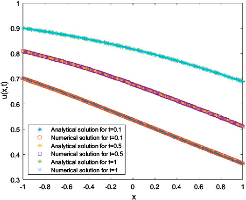
Figure 4. Numerical solution and analytical solution at times $t=0.1,t=0.5,t=1$.

4 Conclusion

This study introduces a novel one-level meshless method for solving the one-dimensional nonlinear Fisher’s equation, leveraging space-time radial basis functions (RBFs). The key findings are summarized as follows:

• The use of space-time RBFs eliminates the requirement for the traditional two-level numerical procedure (e.g., separate time-stepping and spatial discretization), significantly reducing computational complexity.

•The meshless nature of the method avoids reliance on structured grids, making it suitable for problems with complex geometries or dynamic boundaries.

•Numerical experiments demonstrate that the method achieves high accuracy (e.g., compared to analytical solutions) while maintaining low computational costs, particularly for long-term simulations.

In conclusion, the proposed one-level meshless method provides an efficient and flexible numerical tool for solving time-dependent partial differential equations, particularly in terms of simplifying procedures.‌ As a meshfree collocation method, the proposed method has similar limitations with the other collocation methods. Substantial theoretical groundwork, particularly regarding convergence and stability in generalized frameworks, remains unexplored. These aspects will be systematically investigated in future studies.

Data availability statement

The original contributions presented in the study are included in the article/Supplementary Material, further inquiries can be directed to the corresponding authors.

Author contributions

YJ: Validation, Data curation, Funding acquisition, Conceptualization, Supervision, Writing – original draft. FW: Writing – review and editing, Validation, Writing – original draft, Software, Visualization, Conceptualization, Investigation, Methodology. ZS: Conceptualization, Writing – original draft, Writing – review and editing, Resources, Validation, Formal Analysis, Visualization, Data curation.

Funding

The author(s) declare that financial support was received for the research and/or publication of this article. This work is partially supported by University Natural Science Research Project of Anhui Province (Project No. 2023AH050314) and Horizontal Scientific Research Funds in Huaibei Normal University (No. 2024340603000006).

Conflict of interest

The authors declare that the research was conducted in the absence of any commercial or financial relationships that could be construed as a potential conflict of interest.

Generative AI statement

The author(s) declare that no Generative AI was used in the creation of this manuscript.

Publisher’s note

All claims expressed in this article are solely those of the authors and do not necessarily represent those of their affiliated organizations, or those of the publisher, the editors and the reviewers. Any product that may be evaluated in this article, or claim that may be made by its manufacturer, is not guaranteed or endorsed by the publisher.

Supplementary material

The Supplementary Material for this article can be found online at: https://www.frontiersin.org/articles/10.3389/fphy.2025.1616647/full#supplementary-material

References

1. Drábek P, Takáč P. Convergence to travelling waves in Fisher’s population genetics model with a non-Lipschitzian reaction term. J Math Biol (2017) 75:929–72. doi:10.1007/s00285-017-1103-z

PubMed Abstract | CrossRef Full Text | Google Scholar

2. Bruzzone OA, Utgés ME. Analysis of the invasion of a city by Aedes aegypti via mathematical models and Bayesian statistics. Theor Ecol (2022) 15:65–80. doi:10.1007/s12080-022-00528-y

CrossRef Full Text | Google Scholar

3. Macías-Díaz JE. Conciliating efficiency and dynamical consistency in the simulation of the effects of proliferation and motility of transforming growth factor β on cancer cells. Commun Nonlinear Sci (2016) 40:173–88. doi:10.1016/j.cnsns.2016.03.018

CrossRef Full Text | Google Scholar

4. Mittal RC, Rohila R. A study of one dimensional nonlinear diffusion equations by Bernstein polynomial based differential quadrature method. J Math Chem (2017) 55:673–95. doi:10.1007/s10910-016-0703-y

CrossRef Full Text | Google Scholar

5. Bui TTH, van Heijster P, Marangell R. Stability of asymptotic waves in the Fisher–Stefan equation. Physica D (2024) 470:134383. doi:10.1016/j.physd.2024.134383

CrossRef Full Text | Google Scholar

6. Deng D, Hu M. Non-negativity-preserving and maximum-principle-satisfying finite difference methods for Fisher’s equation with delay. Math Comput Simulat (2024) 219:594–622. doi:10.1016/j.matcom.2024.01.013

CrossRef Full Text | Google Scholar

7. Devi A, Yadav OP. Analysis and simulation of the (2 + 1)-dimensional Fisher’s reaction-diffusion equation with higher order finite element method. Numer Heat Tr B- Fund (2024) 1–25. doi:10.1080/10407790.2024.2360637

CrossRef Full Text | Google Scholar

8. Zorsahin GM, Dag I. Exponential B-splines Galerkin method for the numerical solution of the Fisher’s equation. Iran J Sci Technol Trans Sci (2018) 42:2189–98. doi:10.1007/s40995-017-0403-x

CrossRef Full Text | Google Scholar

9. Kırlı E, Irk D. Efficient techniques for numerical solutions of Fisher’s equation using B-spline finite element methods. Comp Appl Math (2023) 42:151. doi:10.1007/s40314-023-02292-z

CrossRef Full Text | Google Scholar

10. Saad KM, Khader MM, Gómez-Aguilar JF, Baleanu D. Numerical solutions of the fractional Fisher’s type equations with Atangana-Baleanu fractional derivative by using spectral collocation methods. Chaos (2019) 29:023116. doi:10.1063/1.5086771

PubMed Abstract | CrossRef Full Text | Google Scholar

11. Wang T, Jiao Y. A fully discrete pseudospectral method for Fisher's equation on the whole line. Appl Numer Math (2017) 120:243–56. doi:10.1016/j.apnum.2017.06.002

CrossRef Full Text | Google Scholar

12. Geeta A, Varun J. A computational approach for solution of one dimensional parabolic partial differential equation with application in biological processes. Ain Shams Eng J (2018) 9:1141–50. doi:10.1016/j.asej.2016.06.013

CrossRef Full Text | Google Scholar

13. Mohammad T, Neeraj D, Vineet KS. Cubic trigonometric B-spline differential quadrature method for numerical treatment of Fisher’s reaction-diffusion equations. Alex Eng J (2018) 57:2019–26. doi:10.1016/j.aej.2017.05.007

CrossRef Full Text | Google Scholar

14. Haifa BJ. On the numerical solution of Fisher's equation by an efficient algorithm based on multiwavelets. AIMS Math (2021) 6:2369–84. doi:10.3934/math.2021144

CrossRef Full Text | Google Scholar

15. Sakina S, Rohul A, Nadeem H, Ali A. Numerical solution of Fisher’s equation through the application of Haar wavelet collocation method. Numer Heat Tr B- Fund (2024) 1–12. doi:10.1080/10407790.2024.2348129

CrossRef Full Text | Google Scholar

16. Mittal RC, Rohila R. A numerical study of the Burgers’ and Fisher’s equations using barycentric interpolation method. Int J Numer Method H (2023) 33:772–800. doi:10.1108/hff-03-2022-0166

CrossRef Full Text | Google Scholar

17. Wang F, Zheng K, Li C, Zhang J. Optimality of the boundary knot method for numerical solutions of 2D Helmholtz-type equations. Wuhan Uni J Nat Sci (2019) 24 (4):314–320. doi:10.1007/s11859-019-1402-x

CrossRef Full Text | Google Scholar

18. Zhang J, Lin J, Wang F, Gu Y. Simulation of antiplane piezoelectricity problems with multiple inclusions by the meshless method of fundamental solution with the LOOCV algorithm for determining sources. Mathematics-Basel (2025) 13:920. doi:10.3390/math13060920

CrossRef Full Text | Google Scholar

19. Lin Y, Wang F. A space-time meshfree method for heat transfer analysis in porous material. Phys Scripta (2024) 99:115274. doi:10.1088/1402-4896/ad8680

CrossRef Full Text | Google Scholar

20. Zhang X, Yao L, Liu J. Numerical study of Fisher’s equation by the RBF-FD method. Appl Math Lett (2021) 120:107195. doi:10.1016/j.aml.2021.107195

CrossRef Full Text | Google Scholar

21. Ju B, Qu W. Three-dimensional application of the meshless generalized finite difference method for solving the extended Fisher–Kolmogorov equation. Appl Math Lett (2023) 136:108458. doi:10.1016/j.aml.2022.108458

CrossRef Full Text | Google Scholar

22. Geeta A, Kiran B, Homan E, Masoumeh K. A comparative study of particle swarm optimization and artificial bee colony algorithm for numerical analysis of Fisher’s equation. Discrete Dyn Nat Soc (2023) 2023:9964744.

Google Scholar

23. Kiran B, Geeta A, Homan E, Masoumeh K. Applications of particle swarm optimization for numerical simulation of Fisher’s equation using RBF. Alex Eng J (2023) 84:316–22.

Google Scholar

24. Chen W, Hong YX, Lin J. The sample solution approach for determination of the optimal shape parameter in the Multiquadric function of the Kansa method. Comput Math Appl (2018) 75:2942–54. doi:10.1016/j.camwa.2018.01.023

CrossRef Full Text | Google Scholar

25. Zhang J, Wang F, Nadeem S, Sun M. Simulation of linear and nonlinear advection-diffusion problems by the direct radial basis function collocation method. Int Commun Heat Mass (2022) 130:105775. doi:10.1016/j.icheatmasstransfer.2021.105775

CrossRef Full Text | Google Scholar

26. Zhang Z, Wang F. The space-time semi-analytical meshless methods for coupled Burgers' equations. Wuhan Univ J Nat Sci (2024) 29:572–8. doi:10.1051/wujns/2024296572

CrossRef Full Text | Google Scholar

27. Jiang Y, Wang F. A novel semi-analytical meshless method for Navier-Stokes equations arising in fractured rock masses. Chin J Phys (2025) 95:1069–77. doi:10.1016/j.cjph.2025.03.007

CrossRef Full Text | Google Scholar