Dynamical interaction network in urban traffic

Introduction: Urban traffic systems transition dynamically between congestion and free-flow states, driven by local interactions between road segments or regions. Understanding how these interactions contribute to congestion, including system-wide congestion, is crucial for effective traffic management. However, existing research has overlooked the dynamical nature of these interactions, which are essential for capturing the changing behavior of urban traffic.

Methods: In this study, we use a pairwise maximum entropy model to infer interaction networks from sliding time windows and analyze their dynamics during typical daily periods: morning peak, noon off-peak, and evening peak.

Results: We find that (1) interaction networks remain stable within each period but exhibit structural shifts between periods, especially between peak and off-peak periods; (2) stable high-strength edges in dynamical interaction network are characterized by long-range and negative interactions; (3) the proportion and modularity of positive interactions, along with the strength of negative interactions, are important structural features that distinguish peak from off-peak hours.

Discussion: These results provide new insights into how local interaction dynamics drive global state transitions in urban traffic, offering guidance for improving traffic resilience through targeted control strategies.

1 Introduction

Urban traffic systems are complex dynamic systems [1], frequently transitioning between congestion and free-flow states. This dynamic nature amplifies the impact of peak-hour demand, leading to extreme congestion that imposes significant societal and economic costs. For example, in 2024, drivers in New York and Chicago lost an average of 102 h and over $1,800 annually due to traffic delays [2]. Understanding the mechanisms behind traffic state transitions is crucial for effective congestion management and urban traffic optimization. Traditional studies have advanced microscale vehicle behavior modeling (e.g., car-following models [3], cellular automata [4]) and macroscale fundamental diagram (MFD) theory [5]. However, these single-scale approaches fail to capture cross-scale emergent behaviors in urban traffic systems, specifically, how local traffic interactions give rise to global congestion.

To bridge this gap, mesoscopic approaches such as percolation theory offer promise for analyzing urban traffic phase transitions. Li et al. [6] use percolation theory to demonstrate how local free-flow components contribute to global connectivity, and further identify critical bottleneck roads whose regulation can significantly improve overall traffic performance. Building on this, Zeng et al. [7] identify different percolation behaviors in peak and off-peak periods: peak-hour networks resemble two-dimensional lattices with short-range interactions, while off-peak networks exhibit small-world properties due to long-range highway connections. In contrast to these studies focusing on free-flow interactions, Duan et al. [8] view congestion propagation between road segments as a tree-like growth process. They find that congestion dissipation duration follows a power-law distribution and that early congestion growth rates correlate with final congestion size, providing early warnings for large-scale jams. Despite these insights, the underlying local interaction mechanisms within urban traffic networks remain incompletely understood.

In terms of modeling interactions within road networks, much of the prior research has focused on local dependencies between road segments during congestion propagation. For example, Li et al. [9] apply spatial correlation analysis to uncover long-range power-law dependencies in congestion propagation, linking them to criticality in overload cascading failures. Nguyen et al. [10] utilize causal congestion trees and dynamic Bayesian networks to model spatiotemporal propagation probabilities, identifying frequent substructures in congestion patterns. Chen et al. [11] propose a Space-Temporal Congestion Subgraph (STCS) framework to model congestion propagation as dynamic graphs. They use temporal-spatial edge-filling strategies to uncover complex patterns in Shanghai Road network, outperforming traditional tree-based models in detecting large-scale recurrent congestion clusters. Further, Luan et al. [12] integrate dynamic Bayesian networks with graph convolutional networks (GCNs) to infer congestion propagation patterns, using data-driven adjacency matrices to capture time-varying relationships between road segments. However, most segment-level interaction inference methods have been applied only to small-scale road networks, limiting their scalability to city-wide systems.

Recent advancements have shifted focus toward regional interactions within urban traffic networks. For instance, Wang et al. [13] propose a POI-guided meta-block to model inter-regional interactions, where regional land-use functions (e.g., commercial, residential) are incorporated into GCN-based traffic prediction. By leveraging self-attention mechanisms, the model dynamically captures spatiotemporal correlations between regions with divergent functions, thereby enabling more accurate predictions of traffic flow across different urban zones. Rajeh et al. [14] develop a Multi-Region Correlation (MRC) framework combined with a Multiple Linear Regression Unit (MLRU) to model the temporal correlations between regions for urban traffic flow prediction. This approach integrates historical traffic data from neighboring regions to improve prediction accuracy, without relying on external factors such as weather or point-of-interest data. While these studies effectively reduce the modeling dimension of large-scale road networks, they primarily focus on region-level traffic flow prediction, with limited exploration of how inter-regional interactions shape the macro-state of the entire system.

In our prior work [15], we used a pairwise maximum entropy model to infer a regional interaction network during a single peak-hour time window. By reconstructing an energy landscape from the inferred regional interaction network, we identified hidden high-risk traffic states. This interaction network highlights both positive interactions (e.g., congestion propagation) and negative interactions (e.g., congestion mitigation) between regions. Unlike other local interaction inference methods, this approach accounts for the collective behavior of the entire system, characterizing how local interactions shape global state distributions. However, urban traffic systems are subject to continuous disturbances that alter local interaction dynamics, shifting the energy landscape and impacting decision-making. The fixed interaction network in our previous research is insufficient to capture such temporal variations. This highlights the need to analyze how interaction networks evolve over time. Building on this, the current study extends our earlier work by examining regional interaction networks across multiple consecutive time windows, including morning peak, noon off-peak, and evening peak periods. Key findings include: (1) interaction networks remain stable within each period but show structural shifts between periods, particularly between peak and off-peak periods; (2) stable high-strength edges in dynamical interaction network are characterized by long-range and negative interactions; (3) the proportion and modularity of positive interactions, along with the strength of negative interactions, are important structural features that distinguish peak from off-peak hours.

The remainder of this paper is structured as follows. Section 2 presents the main results, including interaction networks across traffic periods, macroscopic dynamics of interaction networks, microscopic dynamics of high-strength edges, and evolution of structural features in dynamical interaction network. Section 3 summarizes our research and presents future research directions. Finally, details of the data sources and methods are provided.

2 Results

2.1 Interaction networks across traffic periods

To analyze the dynamical interaction network in urban traffic, this study focuses on the road network within Beijing fourth Ring Road. This road network is divided into 20 predefined hexagonal regions (Figure 1a). We use 1-min interval speed records from floating vehicles collected during 17 workdays in October 2015. Raw speed data from over 33,000 road segments are aggregated to construct a global traffic state for each time step (Figure 1b). Each global traffic state is represented as a 20-dimensional binary vector of regional states, defined by a congestion proportion f and a regional jam threshold l (see Data and methods).

Figure 1

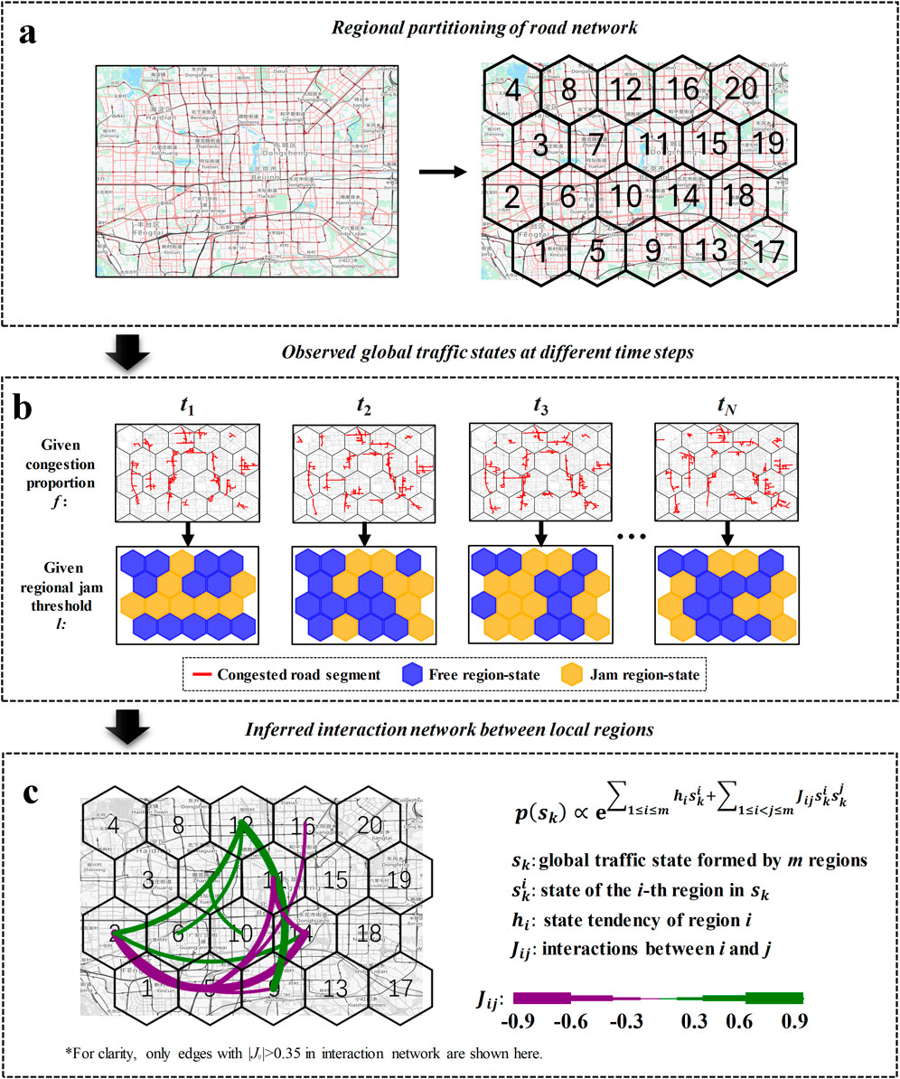
Figure 1. Inference of interaction network in urban traffic using the pairwise maximum entropy model. (a). The road network within Beijing fourth Ring Road is divided into 20 hexagonal regions. (b). Observed global traffic states (see Methods) at different time steps. (c). Interaction network inferred from model parameters [15]. The model input includes observed global traffic states from all time steps within a given time window across 17 workdays. The model outputs (J_ij) are used to build interaction network, where |J_ij| represents the edge strength between regions i and j, and the sign of J_ij indicates whether the interaction between the two regions promotes congestion (J_ij >0) or mitigates congestion (J_ij <0). All maps in this article are from OpenStreetMap.

We apply a pairwise maximum entropy model [15] (Equations 9, 10) to infer regional interaction networks over 24 consecutive 1-h time windows (7:00–18:30, with half-hour sliding intervals). The 24 time windows mentioned below refer to these consecutive 1-h intervals. For each time window, the model input includes global traffic states (Figure 1b) from all time steps within that window over the 17 workdays (see Methods). The resulting interaction network (Figure 1c) consists of nodes representing the 20 predefined road regions (Figure 1a), and edges defined by the inferred model parameters J_ij = J_ji. These interaction networks are weighted and heterogeneous. The absolute value |J_ij| represents interaction strength, and the sign distinguishes mutual congestion propagation (J_ij >0) and mitigation (J_ij <0) [16]. This maximum entropy model infers a local interaction network capturing the statistical distribution of system-level macroscopic performance (Appendix A). By accounting for the collective behavior of the entire system, it characterizes how local interactions shape global state distributions.

Next, we compare interaction networks across traffic periods with different efficiency levels. Traffic efficiency (see Methods) is measured by the mean relative speed $〈v〉$ (Equation 7) and the mean size of the largest functional cluster $〈G〉$ (Equation 8) [6]. These metrics vary considerably across the 24 time windows and display a clear pattern of morning peak, noon off-peak, and evening peak periods (Figure 2d). Based on this, we choose three typical time windows for comparison: 8:00–9:00 in morning peak, 12:00–13:00 in noon off-peak, and 17:30–18:30 in evening peak. As shown in Figures 2a–c, the spatial distributions of the top 5% strongest interaction edges are very different in these three time windows. Compared to noon off-peak period (Figure 2b), peak periods (Figures 2a, c) have more strong positive links, suggesting a greater likelihood of congestion propagation between regions. Moreover, the strong positive links during peak periods tend to cluster in space. For instance, in the morning peak (Figure 2a), Region 5 has strong positive connections with three other regions. In the evening peak (Figure 2c), Region 12 exhibits a similar clustering pattern. This spatial clustering suggests the emergence of critical regions during peak hours. In these regions, localized congestion is more likely to spread and trigger large-scale gridlock [17], thereby reducing overall network efficiency. These findings imply that temporal variations in traffic efficiency (Figure 2d) may be influenced by structural dynamics of the interaction networks. This highlights the need to further investigate their dynamical characteristics, extending the previous model [15] that focusing on a single typical time window.

Figure 2

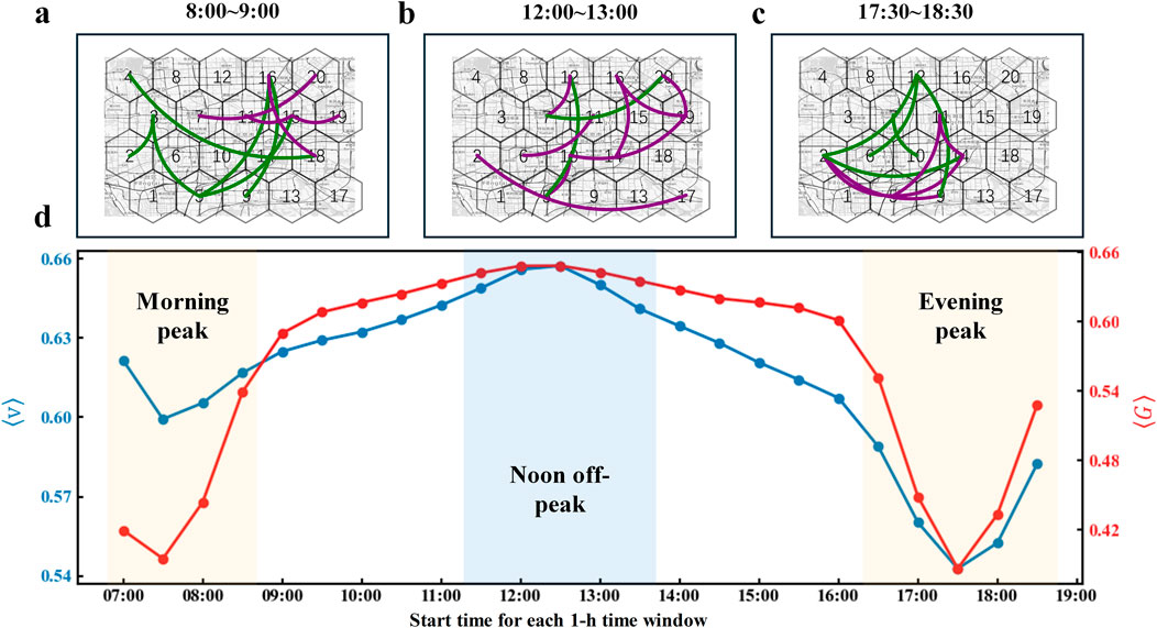
Figure 2. Traffic efficiency and interaction networks across different time windows. (a, b, c). Spatial distributions of the top 5% strongest interaction edges in the 8:00–9:00, 12:00–13:00, and 17:30–18:30 time windows. Green edges indicate positive J_ij, while purple edges indicate negative J_ij. (d). Traffic efficiency varies with the start time of each 1-h time window (7:00–18:30, with half-hour sliding intervals). The morning peak period includes four 1-h time windows (7:00–8:30, with half-hour sliding intervals), the noon off-peak period includes five 1-h time windows (11:30–13:30, with half-hour sliding intervals), and the evening peak period includes five 1-h time windows (16:30–18:30, with half-hour sliding intervals). Traffic efficiency is quantified by the mean relative speed $〈v〉$ and the mean size of the largest functional cluster $〈G〉$, both averaged over all time steps within each 1-h window across 17 workdays (see Methods).

2.2 Macroscopic dynamics of interaction networks

To quantify macroscopic dynamics of interaction networks, we analyze their structural differences across distinct traffic periods. Specifically, we compare interaction networks during the morning peak, noon off-peak, and evening peak periods (Figure 2d), both within and across these periods. Structural dissimilarity is measured using the Jaccard index, which is the ratio of common edges with identical signs to the total number of edges (Equation 11). A low Jaccard index indicates a large structural difference, while a high index suggests great structural similarity. We compute Jaccard indices for all intra-period and inter-period interaction network pairs, generating empirical distributions of these indices. To assess these distributions, we perform a one-tailed Mann-Whitney U test [18] (see Methods) to compare the empirical Jaccard index distribution with that of shuffled edge-sign networks. A one-tailed p-value below the predefined significance level indicates that the empirical Jaccard indices are statistically significantly greater than that of the shuffled networks, suggesting that empirical interaction networks exhibit stronger structural similarity than expected by chance. In addition, we report Cliff’s Δ (Effect size; Equation 12) to quantify the extent to which the structural similarity in empirical interaction networks exceeds that of the shuffled baseline. Larger positive values of Cliff’s Δ indicate a greater proportion of empirical Jaccard indices exceeding those from shuffled networks.

As shown in Figures 3a–c, intra-period interaction networks exhibit significantly high structural similarity, with most Jaccard indices exceeding 0.6 and some surpassing 0.7. Statistical comparisons with shuffled null networks confirm the stability of within-period structures (morning peak: p < 0.001, Cliff’s Δ = 0.905; noon off-peak: p < 0.001, Cliff’s Δ = 0.889; evening peak: p < 0.001, Cliff’s Δ = 0.871). In contrast, inter-period interaction networks show lower Jaccard indices (about 0.5 in Figures 3d–f), indicating greater structural dissimilarity. Notably, peak-off-peak comparisons (Figures 3e, f) show p-values greater than 0.1 and very low effect sizes (Cliff’s Δ < 0.16), providing no statistical evidence that empirical interaction networks exhibit greater structural similarity across peak and off-peak periods than shuffled networks. These results suggest that interaction networks remain stable within each period but show structural shifts between periods, particularly between peak and off-peak periods. High within-period similarity indicates consistent regional interaction patterns, maintaining relatively consistent traffic behavior under stable traffic conditions. In contrast, lower between-period similarity reflects interaction reconfigurations, which drive transitions between distinct traffic states.

Figure 3

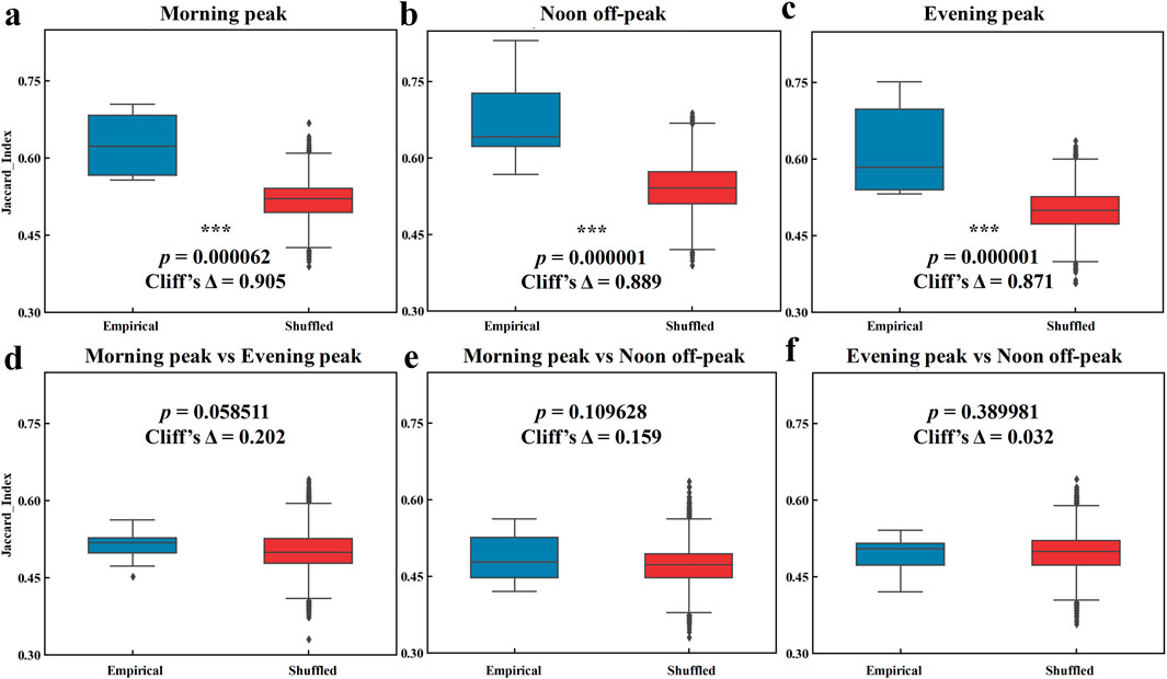
Figure 3. Macroscopic structural differences of interaction networks within and across periods (morning peak, noon off-peak, evening peak). A small Jaccard index indicates great structural difference, while a large index suggests strong similarity. (a, b, c). Intra-period Jaccard index distributions: Jaccard indices for all time window pairs within the same period (a: morning peak; b: noon off-peak; c: evening peak). (d, e, f). Inter-period Jaccard index distributions: Jaccard indices for all time window pairs between different periods (d: morning–evening peak; e: morning peak–noon off-peak; f evening peak–noon off-peak). *Note: Asterisks above distributions denote statistical significance from one-tailed Mann–Whitney U tests (*** = p < 0.001, ** = p < 0.01, * = p < 0.05), comparing empirical Jaccard indices to null distributions generated by 1,000 shuffled edge-sign networks. The one-tailed p-value below the predefined significance level indicates that the empirical Jaccard indices are statistically significantly greater than that of the shuffled networks, suggesting that empirical interaction networks exhibit stronger structural similarity than expected by chance. In addition, we report Cliff’s Δ (Equation 12) to quantify the extent to which the structural similarity in empirical interaction networks exceeds that of the shuffled baseline. Larger positive values of Cliff’s Δ indicate a greater proportion of empirical Jaccard indices exceeding those from shuffled networks (see Methods).

2.3 Microscopic dynamics of high-strength edges

To investigate the microscopic dynamics of interaction networks, we examine the fluctuations of strongly interacting edges over consecutive time windows. First, we rank all edges based on their average interaction strength (⟨|J_ij|⟩) across the 24 time windows. As shown in Figure 4a, edges in the top 30% by ⟨|J_ij|⟩ are considered high-strength edges, while the rest are classified as low-strength edges. The threshold for high-strength edges is ⟨|J_ij|⟩₍₃₀₎ = 0.299, meaning that most edges (70%) have relatively low average interaction strength smaller than that. To quantify the fluctuations of these high-strength edges, we measure two aspects: strength volatility and sign volatility. Strength volatility (CV(|J_ij|) in Equation 13) is the coefficient of variation of |J_ij| across the consecutive time windows, with higher CV(|J_ij|) values indicating greater fluctuations in interaction strength. Sign volatility (SF(J_ij) in Equation 14) is the number of sign flips in J_ij across the consecutive time windows, with more flips indicating higher instability in interaction sign.

Figure 4

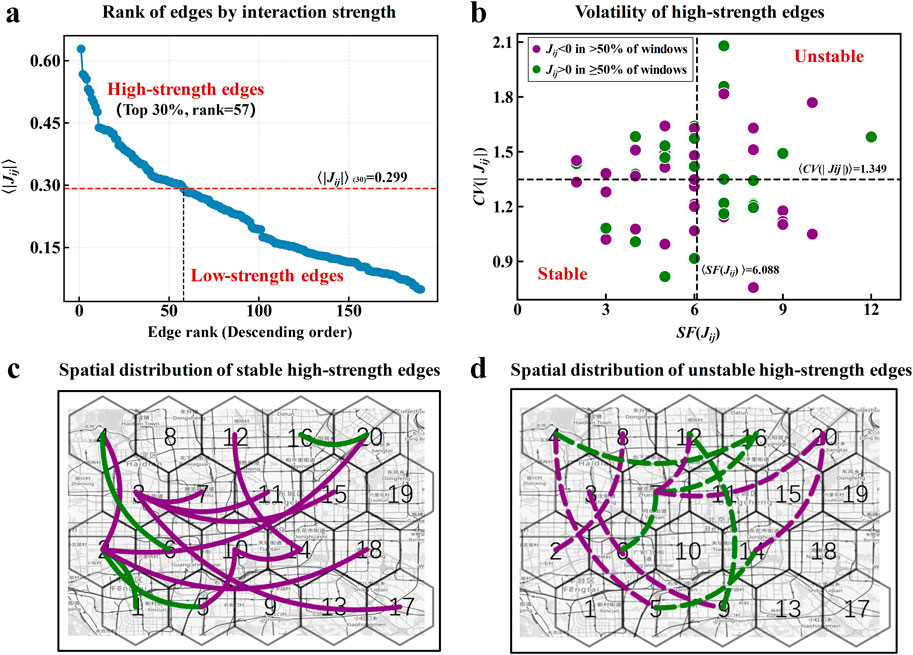
Figure 4. Microscopic edge dynamics in interaction networks across consecutive time windows. (a). Rank of edges by the mean of |J_ij| (denoted as ⟨|J_ij|⟩) across multiple time windows. Here, the 24 time windows covering morning peak, noon off–peak, and evening peak periods are selected to analyze edge dynamics. Edges in the top 30% by ⟨|J_ij|⟩ are classified as high-strength edges, while the rest are low-strength edges. The threshold ⟨|J_ij|⟩₍₃₀₎ = 0.299 is marked by the red dashed line. (b). Volatility of high–strength edges. The mean coefficient of variation (⟨CV(|J_ij|)⟩ = 1.349) is used as the threshold for strength volatility, and the mean number of sign flips (⟨SF(J_ij)⟩ = 6.088) as the threshold for sign volatility, both marked by black dashed lines. High-strength edges with CV(|J_ij|)≥⟨CV(|J_ij|)⟩ and SF(J_ij)≥⟨SF(J_ij)⟩ are classified as unstable high-strength edges, while those with CV(|J_ij|) < ⟨CV(|J_ij|)⟩ and SF(J_ij) < ⟨SF(J_ij)⟩ are classified as stable high-strength edges. (c, d). Spatial distributions of stable and unstable high-strength edges. Green edges indicate those with J_ij >0 in at least half of the 24 time windows (i.e., consistently positive interactions), while purple edges indicate those with J_ij <0 in more than half of the 24 time windows (i.e., consistently negative interactions).

As shown in Figure 4b, high-strength edges exhibit a wide range of both strength and sign volatility. Specifically, CV(|J_ij|) ranges from 0.8 to 2.1, while SF(J_ij) ranges from 2 to 12. We classify edges as stable if both volatility measures are below their mean values, and as unstable if both volatility measures are greater than or equal to their mean values. Among these high-strength edges, stable edges account for 24.6%, while unstable edges make up 19.3%. Notably, stable high-strength edges have a higher proportion of negative interactions occurring in more than 50% of the time windows (purple points in Figure 4b), compared to unstable high-strength edges. This indicates that stable high-strength edges consistently suppress congestion. Spatial analysis further reveals that some stable negative high-strength edges (e.g., edge between regions 3 and 17 in Figure 4c) span longer distances than unstable ones (Figure 4d). These long-range, negative-effect stable edges form a geographically dispersed network. Showing negative interactions across distant regions, they may reflect negative feedbacks to prevent congestion from spreading into widespread gridlock [17], demonstrating the inherent resilience [19] of urban traffic.

2.4 Evolution of structural features in dynamical interaction network

After analyzing the dynamics of macroscopic structure and microscopic edge, we further investigate the evolution of structural features in dynamical interaction network. We quantify this evolution using four structural metrics (denoted as $P_{+}$, $P_{+}^s$, $Q_p^w$, and ${〈k〉}_n^w$; see Methods), which capture both network-level and node-level properties of the weighted and heterogeneous interaction networks. For each of the 24 interaction networks (corresponding to the 24 time windows), we compute these metrics, which reveal distinct temporal patterns and exhibit strong interpretability (Figure 5).

Figure 5

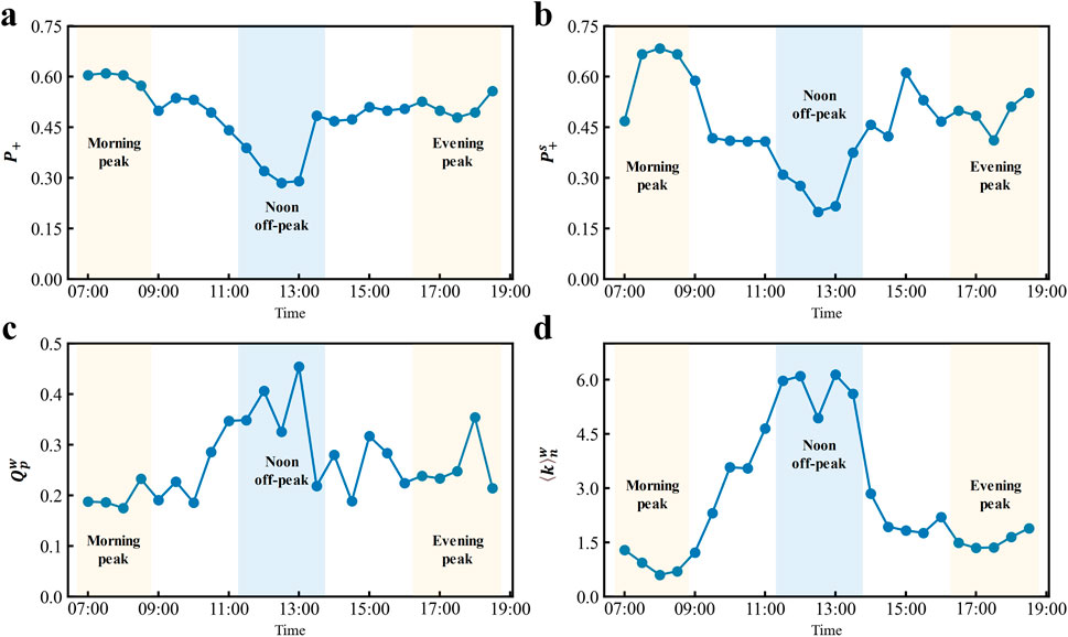
Figure 5. Evolution of four structural features in dynamical interaction networks. These four structural features (see Method), including $P_{+}$ (a), $P_{+}^s$ (b), $Q_p^w$ (c), and ${〈k〉}_n^w$ (d), exhibit temporal variation across the 24 time windows. All four metrics show clear differences among the morning peak, noon off-peak, and evening peak periods.

The proportion of positive interactions ($P_{+}$; Equation 15) quantifies the overall positive polarity of interactions within the network. A higher $P_{+}$ value indicates more mutual reinforcement between regions, increasing the likelihood of congestion propagation. As shown in Figure 5a, $P_{+}$ is significantly higher during the morning and evening peak hours compared to noon off-peak. Specifically, $P_{+}$ reaches approximately 0.6 in the morning peak, 0.5 in the evening peak, and 0.3 during noon off-peak. This suggests that peak hours have more positive interactions, facilitating congestion spread. A similar trend is observed for the proportion of strong positive interactions ($P_{+}^s$, calculated from subnetwork with |J_ij| >0.2): peak values are much higher than off-peak (Figure 5b), enhancing congestion spread effects.

The weighted modularity of positive interactions ($Q_p^w$; Equation 16) reflects whether positive links tend to form community-like structures. A higher $Q_p^w$ value implies that congestion propagation is more likely to remain within specific regional clusters rather than spread globally. As shown in Figure 5c, $Q_p^w$ is much higher during noon off-peak compared to peak hours. Most $Q_p^w$ values are around 0.4 during noon off-peak, while they are about 0.2 during peak hours. This indicates that positive interactions during off-peak periods are more likely to form community structures, helping to confine congestion within local regions. In contrast, during peak hours, positive interactions are less likely to form such structures, resulting in widespread congestion.

The average node strength of negative interactions (${〈k〉}_n^w$; Equation 17) represents the strength of inhibitory effects between regions. A higher ${〈k〉}_n^w$ signifies stronger suppression of congestion. As shown in Figure 5d, ${〈k〉}_n^w$ is lower during peak hours (around 1.5) and higher during off-peak hours (approaching 6.0). This demonstrates that inhibitory effects of regions are significantly stronger during off-peak periods, preventing congestion from spreading between regions.

Our findings reveal that the proportion and modularity of positive interactions, along with the strength of negative interactions, are important structural features distinguishing peak from off-peak hours. During peak hours, the network is dominated by a high proportion and low modularity of positive interactions, along with weak inhibitory interactions. These structural characteristics reduce the ability of the interaction network to localize congestion, leading to large-scale traffic congestion. In contrast, off-peak periods are characterized by a low proportion and high modularity of positive interactions, and strong inhibitory effects, which help localize congestion and maintain overall traffic efficiency.

3 Discussion

This study extends our previous work [15], which used a pairwise maximum entropy model to infer a regional interaction network for a single peak-hour time window and identify hidden high-risk states through energy landscape reconstruction. While [15] characterized static interactions during peak congestion, it overlooked dynamic evolutions of interaction networks across periods with varying traffic efficiency (morning peak, noon off-peak, evening peak). These variations can reshape energy landscapes and impact risk-based decision-making. Here, we apply the pairwise maximum entropy model to multiple consecutive time windows, analyzing dynamical interaction networks to derive three key findings.

First, interaction networks remain stable within each period (morning peak, noon off-peak, and evening peak), but show structural shifts between periods, especially between peak and off-peak hours. High similarity of within-period network structure indicates consistent regional interaction patterns, maintaining traffic behavior. In contrast, lower between-period similarity reflects structural reconfigurations, which likely drive transitions between distinct traffic states [20]. Second, compared with unstable high-strength edges, stable high-strength edges in dynamical interaction network are characterized by long-range and negative interactions. These interactions help suppress congestion spread across distant regions. This prevents localized congestion from turning into widespread gridlock [17] and highlights the inherent resilience [19] of urban traffic. Third, the proportion and modularity of positive interactions, along with the strength of negative interactions, are important structural features that distinguish peak from off-peak hours. Compared to off-peak periods, peak hours feature a higher proportion and lower modularity [21] of positive interactions, along with weaker inhibitory effects, which may lead to large-scale congestion.

These findings address the limitations of our prior study [15], which applied a static analysis of interaction networks during a single peak-hour time window and overlooked the dynamic evolution of interactions across different traffic periods. The discovery that interaction networks remain stable within individual periods (e.g., morning peak, noon off-peak) but undergo structural shifts between periods emphasizes the importance of temporal dynamics in reshaping the energy landscape, a factor not captured in static models. Furthermore, the identification of long-range negative interactions as the dominant feature of stable high-strength edges in dynamic networks uncovers a key resilience mechanism—the suppression of congestion spread across distant regions—which was undetected in the prior static model. Additionally, the differentiation of peak and off-peak periods based on structural features such as positive interaction modularity and negative interaction strength introduces the temporal context missing in our previous work, enabling a deeper understanding of how interaction configurations contribute to macroscale congestion transitions.

While these findings enhance our understanding of dynamical interaction network underlying traffic state transitions, there are still several limitations. First, the model relies on predefined time window data and may perform poorly in extreme scenarios [22] (e.g., sudden demand surges or infrastructure failures) due to data scarcity. Second, the analysis focuses on a regional scale and may not capture finer-scale local interaction complexity. As urban traffic systems are complex and multiscale [23], these findings might not directly apply to interaction networks with higher spatial resolution. Future research should develop multi-scale adaptive models [24] to capture interactions across local road network scales and adapt to data-scarce extremes. These models may reflect inherent robustness in real-world applications, particularly as autonomous driving [25] and other technologies reshape local interaction patterns.

4 Data and methods

4.1 Data

4.1.1 Raw traffic dataset

The empirical road network in this study covers the area within Beijing fourth Ring Road (Figure 1a). Road segments are modeled as edges and intersections as nodes, with the network comprising over 18,000 nodes and 33,000 edges. The dataset includes 1-min interval speed records from GPS-equipped floating vehicles across all workdays in October 2015, excluding October 19 due to data anomalies. This results in 17 valid workdays. To account for road type heterogeneity, we use relative velocity instead of raw speed values. As defined in [6], the relative velocity of a segment e at time t is computed as the ratio of its observed speed to its standard maximum speed, defined as the 95th percentile of its historical daily speed records:

$v_e\left(t\right)=\frac{u_e\left(t\right)}{u_e^{free}},(1)$

where $u_e\left(t\right)$ is the observed speed of segment e at time t, and $u_e^{free}$ denotes the 95th percentile of daily speed records for segment e.

4.2 Data pre-processing

To study the interactions between local components of the road network, we focus on regional interactions rather than segment-level interactions to avoid combinatorial explosion in state space. Following our previous work [15], we divide the entire road network into 20 hexagonal regions (Figure 1a), and aggregate road segment states into global traffic states for each time step. The aggregation procedure is as follows.

4.2.1 Segment-level state (congestion proportion f)

For each road segment e at time t, we define its state based on the relative velocity $v_e\left(t\right)$ (Equation 1). Given a congestion proportion threshold f, we mark the bottom f × 100% of segments (by relative velocity) as congested at time t, and the rest as non-congested. The value of f represents the proportion of congested roads in the network, influencing its performance distribution. Based on the discovery of the multi-stability phenomenon in Beijing Road network [20], when f is high (e.g., >0.4), most roads are congested, resulting in a poor steady state. When f is low (e.g., <0.2), most roads are uncongested, leading to a good steady state. When f is between 0.2 and 0.4, the network exhibits multiple steady states due to the varying spatial distributions of congested links over time. This multi-stability reflects the inner system resilience [20]. Here, we chose f = 0.25, as it lies in this range, with the model showing robustness for other values within this interval, as demonstrated in [15].

4.2.2 Region-level state (regional jam threshold l)

For region i at time t, we calculate the jam ratio based on the congested segments in that region, which is defined as:

$r_i\left(t\right)=\frac{C_i^{con}\left(t\right)}{N_i},(2)$

where $N_i$ is the total number of road segments in region i, and $C_i^{con}\left(t\right)$ is the number of congested segments in the largest connected cluster formed by congested segments at time t. If the jam ratio (Equation 2) exceeds a threshold l, the region is classified as a jam region; otherwise, it is classified as a free region. The state of region i at time t is:

$s_i\left(t\right)=\left\{\begin{array}{l}1,\text{if}{r}_i\left(t\right)>l\left(\text{jam region}\right)\\ -1,\text{otherwise}\left(\text{free region}\right)\end{array}\right..(3)$

Here, we set l to be 0.09. The value of l represents the threshold for the maximum congestion cluster within each region. It influences the system performance distribution at mesoscopic level. When l is large, all regions are considered free, resulting in the performance distribution concentrated in a better state at the mesoscopic level. When l is small, all regions are jam, leading to the performance distribution concentrated in a worse state. At l = 0.09, the mesoscopic network performance shows multi-stability, aligning closely with the performance at the microscopic level, as shown in [15].

4.2.3 Global traffic state

At time t, the global traffic state is represented as a binary vector over all regions:

$s\left(t\right)=\left\{s^1\left(t\right),s^2\left(t\right),\dots ,s^i\left(t\right),{\dots ,s}^{20}\left(t\right)\right\},(4)$

where $s^i\left(t\right)\in \left\{1,-1\right\}$.

5 Methods

5.1 Traffic efficiency of each time window

To quantify the traffic efficiency of each 1-h time window, we compute two metrics: the mean relative speed $〈v〉$, reflecting overall traffic conditions, and the mean size of the largest functional cluster $〈G〉$, which captures the interplay between traffic dynamics and road network topology [6]. Both metrics are averaged over all time steps within a given time window across 17 workdays.

For a given time step t, we define.

(1) Average relative speed v(t) as the mean of the relative velocities of all road segments:

$v\left(t\right)=\frac{1}{N_E}{\displaystyle \sum _{e=1}^{N_E}}{v}_e\left(t\right),(5)$

where $N_E$ is the total number of road segments, and $v_e\left(t\right)$ is the relative velocity (Equation 1) of road segment e at time t.

(2) Size of the largest functional cluster G(t) as the proportion of road segments in the largest functional cluster formed by non-congested segments:

$G\left(t\right)=\frac{C^{non}\left(t\right)}{N_E},(6)$

where $C^{non}\left(t\right)$ is the number of segments in the largest functional cluster formed by non-congested segments at time t.

Based on Equations 5, 6, the aggregate metrics for each time window are then computed as:

$〈v〉=\frac{1}{T}{\displaystyle \sum _{t\in \mathrm{T}}}v\left(t\right),(7)$

$〈G〉=\frac{1}{T}{\displaystyle \sum _{t\in \mathrm{T}}}G\left(t\right),(8)$

where T is the set of all time steps within the time window across all 17 workdays, and $T=\left|\mathrm{T}\right|$ is the total number of such time steps.

5.2 Interaction network inference through pairwise maximum entropy model

Here, we infer the interaction network between regions for each time window using a pairwise maximum entropy model [15]. This model has been applied to neuron interaction network [16], brain functional connectivity [26], and genetic interaction networks [27]. The model maximizes (Gibbs) entropy under constraints of first- and second-order statistics, yielding the probability distribution $p\left(s_k\right)$:

$\begin{array}{l}\begin{array}{cc}\max & H=-{\displaystyle \sum _{1\le k\le n}}p\left(s_k\right)\log p\left(s_k\right)\end{array}\\ \begin{array}{cc}\mathrm{s}.\mathrm{t}.& \begin{array}{l}{\displaystyle \sum _{1\le k\le n}}p\left(s_k\right)=1\\ \begin{array}{cc}{\displaystyle \sum _{1\le k\le n}}p\left(s_k\right)s_k^i={\displaystyle \sum _{s_d\in D}}f\left(s_d\right)s_d^i,& 1\le i\le m\end{array}\\ \begin{array}{cc}{\displaystyle \sum _{1\le k\le n}}p\left(s_k\right)s_k^i{s}_k^j={\displaystyle \sum _{s_d\in D}}f\left(s_d\right)s_d^i{s}_d^j,& 1\le i<j\le m\end{array}\end{array}\end{array}\end{array},(9)$

where the state space consists of n = 2^m possible states, with m = 20 representing the number of road network regions, and k denoting a particular state within this space. Specifically, $s_k$ represents a global traffic state vector (Equation 4) composed of the states of 20 regions, where $s_k^i=1$ indicates a jam region and $s_k^i=-1$ indicates a free region (Equation 3). $s_d$ and $f\left(s_d\right)$ denote observed global traffic states and their frequencies in dataset D. Solving the Lagrange function yields the Boltzmann distribution:

$p\left(s_k\right)=\left(1/Z\right){\mathrm{e}}^{{\displaystyle \sum _{1\le i\le m}}{h}_i{s}_k^i+{\displaystyle \sum _{1\le i<j\le m}}{J}_{ij}{s}_k^i{s}_k^j},(10)$

where h_i captures the regional congestion tendency of region i, J_ij quantifies the pairwise interaction between regions i and j, and Z is the partition function ${\displaystyle {\sum }_{1\le k\le n}}{\mathrm{e}}^{{\displaystyle {\sum }_{1\le i\le m}}{h}_i{s}_k^i+{\displaystyle {\sum }_{1\le i<j\le m}}{J}_{ij}{s}_k^i{s}_k^j}$.

For each 1-h time window (e.g., 8:00–9:00), we construct a dataset D comprising global traffic states obtained from 60 time steps within the window across 17 workdays. We then compute the empirical moments ${\displaystyle {\sum }_{s_d\in D}}f\left(s_d\right)s_d^i$ and ${\displaystyle {\sum }_{s_d\in D}}f\left(s_d\right)s_d^i{s}_d^j$​. These moments are used to ensure that the resulting distribution $p\left(s_k\right)$ in Equation 10 satisfies the moment constraints specified in Equation 9. The inferred model parameters J_ij are used to define the regional interaction network. Due to the intractability of the state space (2²⁰), we approximate parameter estimation using the minimum probability flow (MPF) algorithm [28].

Model validation evaluates the model ability to reproduce distribution of macroscopic traffic properties [15], such as region-level traffic performance. This performance is defined as the proportion of regions in the largest connected cluster formed by free regions, relative to total regions. As shown in Appendix A, the model accurately fits the 24 time windows, and captures unimodal or bimodal patterns in region-level traffic performance distributions.

5.3 Structural dissimilarity quantification of interaction networks

To quantify structural dissimilarity of interaction networks within the same period (intra-period) or across different periods (inter-period), we calculate the Jaccard indices for all interaction network pairs and compare their distributions with the null distribution generated by shuffled networks.

5.3.1 Jaccard index calculation

The Jaccard index between two interaction networks A and B is calculated as follows:

$J\left(A,B\right)=\frac{\left|\left\{\left(i,j\right)\in E_A\cap E_B|\text{sign}\left(J_{ij}^A\right)=\text{sign}\left(J_{ij}^B\right)\right\}\right|}{\left|E_A\cup E_B\right|},(11)$

where $E_A$ and $E_B$ are the edge sets of interaction networks A and B, respectively; $\text{sign}\left(J_{ij}^A\right)$ and $\text{sign}\left(J_{ij}^B\right)$ denote the signs of J_ij in A and B, respectively, with the sign being +1 when J_ij is positive and −1 otherwise. The numerator is the number of common edges with the same sign in both networks, and the denominator is the total number of edges in the union of both networks. Only the signs of edges are considered in the calculation, while the weights of edges are ignored. A smaller Jaccard index indicates a greater structural difference between two networks, while a larger Jaccard index suggests more structural similarity between networks.

5.3.2 Statistical significance testing

To assess the structural similarity of interaction networks, we use both p-value and Cliff’s Δ (Effect Size). The p-value assesses statistical significance of structural similarity, while Cliff’s Δ quantifies the magnitude of structural similarity. Specifically, we perform significance testing of Jaccard index distributions derived from two scenarios.

• Intra-period similarity: Given $n_1$ time windows within the same period, we construct $n_1\left(n_1-1\right)/2$ unique interaction network pairs. Next, we compute the Jaccard indices (Equation 11) of these pairs to obtain the empirical intra-period Jaccard index distribution. To generate shuffled interaction network pairs, we randomly shuffle the edge signs of each network pair 1,000 times while preserving edge weights and topology. Calculating the Jaccard indices of these shuffled pairs yields a null distribution of $1000\times n_1\left(n_1-1\right)/2$ Jaccard indices.

• Inter-period similarity: Given two periods with $n_1$ and $n_2$ time windows respectively, we construct $n_1{n}_2$ cross-period network pairs. The empirical Jaccard indices of these pairs form the inter-period Jaccard index distribution. Analogously, a null distribution of $1000\times n_1{n}_2$ Jaccard indices is generated by performing sign shuffling 1,000 times on each network pair.

5.3.2.1 P-value calculation

To assess whether the empirical interaction networks exhibit stronger structural similarity than expected by chance, we perform a one-tailed Mann–Whitney U test [18] comparing the distribution of Jaccard indices computed between empirical networks with that computed between shuffled networks.

• Null hypothesis (H₀): The Jaccard index distributions of the empirical and shuffled interaction networks are drawn from the same population.

• Alternative hypothesis (H₁): The empirical Jaccard indices are stochastically greater than the shuffled ones.

If the one-tailed p-value derived from the test is smaller than the pre-defined significance level, we reject the null hypothesis. This indicates that the Jaccard index distribution of the empirical interaction networks is statistically significantly greater than that of the shuffled networks, suggesting that empirical interaction networks exhibit stronger structural similarity than expected by chance.

5.3.3 Cliff’s Δ (effect size)

In addition to the p-value, we compute Cliff’s Δ as a non-parametric effect size measure to quantify the degree of separation between two distributions. Specifically:

$\text{Clif}{\mathrm{f}}^{\prime }\mathrm{s}\Delta =\frac{N_{C>D}-N_{C<D}}{n_C·n_D},(12)$

where $N_{C>D}$ and $N_{C<D}$ are the number of times a Jaccard index in sample C (the empirical Jaccard index distribution) is greater than or less than a Jaccard index in distribution D (the shuffled Jaccard index distribution), respectively. $n_C$ and $n_D$ are the sizes of the two samples. A large positive Δ indicates that Jaccard indices in C tend to be large than those in D, suggesting strong structural similarity in the empirical network.

5.3.4 Edge volatility

To analyze the edge dynamics across consecutive time windows, two aspects are considered: strength and sign. Here, we use the 24 time windows, covering morning peak, noon off-peak, and evening peak periods. For each edge (i, j), we calculate the following two indicators.

5.3.4.1 Strength volatility

Strength volatility quantifies the relative variability of interaction strengths over time. It is measured using the coefficient of variation:

$CV\left(\left|J_{ij}\right|\right)=\frac{\text{std}\left(\left|J_{ij}\right|\right)}{\text{mean}\left(\left|J_{ij}\right|\right)},(13)$

where the absolute value |J_ij| quantifies interaction strength. A high $CV\left(\left|J_{ij}\right|\right)$ value indicates great fluctuations in the strength of edge (i, j).

5.3.4.2 Sign volatility

Sign volatility measures the number of times the sign of an edge changes (positive to negative or vice versa) across consecutive time windows:

$SF\left(J_{ij}\right)={\displaystyle \sum _{T=1}^{T_n-1}}{1}_{\text{sign}\left(J_{ij}^{\left(T\right)}\right)\ne \text{sign}\left(J_{ij}^{\left(T+1\right)}\right)},(14)$

where $T_n$ is the number of consecutive time windows. A high SF(J_ij) value indicates great fluctuations in the sign of edge (i, j).

5.4 Structural metrics of interaction network

To characterize the weighted and heterogeneous properties of interaction networks, we define four structural metrics that reflect topological aspects such as interaction polarity, modularity, and node connectivity. These include both network-level and node-level metrics.

5.4.1 Network-level metrics

5.4.1.1 Proportion of positive interactions

The proportion of positive interactions ($P_{+}$; Equation 15) is calculated as:

$P_{+}=\frac{N_{edge}^{+}}{N_{edge}},(15)$

where $N_{edge}^{+}$ is the number of edges with J_ij >0, and $N_{edge}$ is the total number of edges in the interaction network. We also define a variant, $P_{+}^s$, computed for the subnetwork with strong interactions where |J_ij| >0.2.

5.4.1.2 Weighted modularity of positive interactions

To quantify the modular structure of positive interactions, we compute the weighted modularity for the subnetwork consisting only of positive interactions (J_ij >0), defined as:

$Q_p^w=\frac{1}{2M_p}\sum _{i,j:J_{ij}>0}\left(J_{ij}-\frac{k_i^w{k}_j^w}{2M_p}\right)\delta \left(c_i,c_j\right),(16)$

where $M_p=\frac{1}{2}{\sum }_{i,j:J_{ij}>0}{J}_{ij}$ is the total positive edge weight, $k_i^w={\sum }_{j:J_{ij}>0}{J}_{ij}$ is the positive strength of node i, and $\delta \left(c_i,c_j\right)$ = 1 if nodes i and j are in the same community [29] of the subnetwork with J_ij>0, and 0 otherwise. A high $Q_p^w$ indicates a strong community structure within the network of positive interactions.

5.4.2 Node-level metrics

5.4.2.1 Average node strength of negative interactions

The average node strength for negative interactions ${〈k〉}^w$ is calculated as:

${〈k〉}_n^w=\frac{1}{N_{node}}\sum _i\sum _j\left|J_{ij}\right|,\text{for}{J}_{ij}<0(17)$

where $N_{node}$ is the number of nodes in the interaction network. This metric captures the average magnitude of negative interaction strength per node.

Data availability statement

The raw data supporting the conclusions of this article will be made available by the authors, without undue reservation.

Author contributions

SL: Investigation, Conceptualization, Writing – review and editing, Visualization, Resources, Formal Analysis, Writing – original draft, Methodology, Validation, Software. GZ: Methodology, Validation, Supervision, Formal Analysis, Writing – review and editing. RL: Methodology, Validation, Writing – review and editing, Formal Analysis, Supervision. LG: Validation, Writing – review and editing, Formal Analysis, Methodology. DL: Writing – original draft, Funding acquisition, Writing – review and editing, Resources, Investigation, Project administration, Conceptualization, Supervision, Formal Analysis, Methodology, Data curation.

Funding

The author(s) declare that financial support was received for the research and/or publication of this article. This work is supported by the National Natural Science Foundation of China (Grants 72225012, 72288101 and 71822101), the Fundamental Research Funds for the Central Universities.

Conflict of interest

The authors declare that the research was conducted in the absence of any commercial or financial relationships that could be construed as a potential conflict of interest.

Generative AI statement

The author(s) declare that no Generative AI was used in the creation of this manuscript.

Publisher’s note

All claims expressed in this article are solely those of the authors and do not necessarily represent those of their affiliated organizations, or those of the publisher, the editors and the reviewers. Any product that may be evaluated in this article, or claim that may be made by its manufacturer, is not guaranteed or endorsed by the publisher.

References

1. Liu C, Yang Y, Chen B, Cui T, Shang F, Fan J, et al. Revealing spatiotemporal interaction patterns behind complex cities. Chaos: Interdiscip J Nonlinear Sci (2022) 32:081105. doi:10.1063/5.0098132

PubMed Abstract | CrossRef Full Text | Google Scholar

2. INRIX. INRIX global traffic scorecard (2024). Available online at: https://inrix.com/scorecard/.

Google Scholar

3. Chandler RE, Herman R, Montroll EW. Traffic dynamics: studies in car following. Operations Res (1958) 6:165–84. doi:10.1287/opre.6.2.165

CrossRef Full Text | Google Scholar

4. Barlovic R, Santen L, Schadschneider A, Schreckenberg M. Metastable states in cellular automata for traffic flow. Eur Phys J B (1998) 5(5):793–800. doi:10.1007/s100510050504

CrossRef Full Text | Google Scholar

5. Geroliminis N, Daganzo CF. Existence of urban-scale macroscopic fundamental diagrams: some experimental findings. Transportation Res B: Methodological (2008) 42:759–70. doi:10.1016/j.trb.2008.02.002

CrossRef Full Text | Google Scholar

6. Li D, Fu B, Wang Y, Lu G, Berezin Y, Stanley HE, et al. Percolation transition in dynamical traffic network with evolving critical bottlenecks. Proc Natl Acad Sci USA (2015) 112:669–72. doi:10.1073/pnas.1419185112

PubMed Abstract | CrossRef Full Text | Google Scholar

7. Zeng G, Li D, Guo S, Gao L, Gao Z, Stanley HE, et al. Switch between critical percolation modes in city traffic dynamics. Proc Natl Acad Sci USA (2019) 116:23–8. doi:10.1073/pnas.1801545116

PubMed Abstract | CrossRef Full Text | Google Scholar

8. Duan J, Zeng G, Serok N, Li D, Lieberthal EB, Huang H-J, et al. Spatiotemporal dynamics of traffic bottlenecks yields an early signal of heavy congestions. Nat Commun (2023) 14:8002. doi:10.1038/s41467-023-43591-7

PubMed Abstract | CrossRef Full Text | Google Scholar

9. Li D, Jiang Y, Kang R, Havlin S. Spatial correlation analysis of cascading failures: congestions and blackouts. Scientific Rep (2014) 4:5381. doi:10.1038/srep05381

CrossRef Full Text | Google Scholar

10. Nguyen H, Liu W, Chen F. Discovering congestion propagation patterns in spatio-temporal traffic data. IEEE Trans Big Data (2017) 3:169–80. doi:10.1109/TBDATA.2016.2587669

CrossRef Full Text | Google Scholar

11. Chen Z, Yang Y, Huang L, Wang E, Li D. Discovering urban traffic congestion propagation patterns with taxi trajectory data. IEEE Access (2018) 6:69481–91. doi:10.1109/access.2018.2881039

CrossRef Full Text | Google Scholar

12. Luan S, Ke R, Huang Z, Ma X. Traffic congestion propagation inference using dynamic Bayesian graph convolution network. Transportation Res C: Emerging Tech (2022) 135:103526. doi:10.1016/j.trc.2021.103526

CrossRef Full Text | Google Scholar

13. Wang K, Liu L, Liu Y, Li G, Zhou F, Lin L. Urban regional function guided traffic flow prediction. Inf Sci (2023) 634:308–20. doi:10.1016/j.ins.2023.03.109

CrossRef Full Text | Google Scholar

14. Rajeh TM, Li T, Li C, Javed MH, Luo Z, Alhaek F. Modeling multi-regional temporal correlation with gated recurrent unit and multiple linear regression for urban traffic flow prediction. Knowledge-Based Syst (2023) 262:110237. doi:10.1016/j.knosys.2022.110237

CrossRef Full Text | Google Scholar

15. Liu S, Bai M, Guo S, Gao J, Sun H, Gao Z-Y, et al. Hidden high-risk states identification from routine urban traffic. PNAS nexus (2025) 4:pgaf075. doi:10.1093/pnasnexus/pgaf075

PubMed Abstract | CrossRef Full Text | Google Scholar

16. Schneidman E, Berry MJ, Segev R, Bialek W. Weak pairwise correlations imply strongly correlated network states in a neural population. Nature (2006) 440:1007–12. doi:10.1038/nature04701

PubMed Abstract | CrossRef Full Text | Google Scholar

17. Mahmassani HS, Saberi M, Zockaie A. Urban network gridlock: theory, characteristics, and dynamics. Procedia-Social Behav Sci (2013) 80:79–98. doi:10.1016/j.sbspro.2013.05.007

CrossRef Full Text | Google Scholar

18. Shier R Statistics: 2.3 the Mann-Whitney u test. In: Mathematics learning support centre (2013).

Google Scholar

19. Zhang L, Zeng G, Li D, Huang H-J, Stanley HE, Havlin S. Scale-free resilience of real traffic jams. Proc Natl Acad Sci USA (2019) 116:8673–8. doi:10.1073/pnas.1814982116

PubMed Abstract | CrossRef Full Text | Google Scholar

20. Zeng G, Gao J, Shekhtman L, Guo S, Lv W, Wu J, et al. Multiple metastable network states in urban traffic. Proc Natl Acad Sci USA (2020) 117:17528–34. doi:10.1073/pnas.1907493117

PubMed Abstract | CrossRef Full Text | Google Scholar

21. Shi D, Shang F, Chen B, Expert P, Lü L, Stanley HE, et al. Local dominance unveils clusters in networks. Commun Phys (2024) 7:170–13. doi:10.1038/s42005-024-01635-4

CrossRef Full Text | Google Scholar

22. Gao S, Li D, Zheng N, Hu R, She Z. Resilient perimeter control for hyper-congested two-region networks with MFD dynamics. Transportation Res Part B: Methodological (2022) 156:50–75. doi:10.1016/j.trb.2021.12.003

CrossRef Full Text | Google Scholar

23. Guo Q, Ban X. Network multiscale urban traffic control with mixed traffic flow. Transportation Res Part B: Methodological (2024) 185:102963. doi:10.1016/j.trb.2024.102963

CrossRef Full Text | Google Scholar

24. Dada JO, Mendes P. Multi-scale modelling and simulation in systems biology. Integr Biol (2011) 3:86–96. doi:10.1039/c0ib00075b

PubMed Abstract | CrossRef Full Text | Google Scholar

25. He W, Chen W, Tian S, Zhang L. Towards full autonomous driving: challenges and frontiers. Front Phys (2024) 12. doi:10.3389/fphy.2024.1485026

CrossRef Full Text | Google Scholar

26. Watanabe T, Hirose S, Wada H, Imai Y, Machida T, Shirouzu I A pairwise maximum entropy model accurately describes resting-state human brain networks. Nat Commun (2013) 4:1370. doi:10.1038/ncomms2388

PubMed Abstract | CrossRef Full Text | Google Scholar

27. De Martino A, De Martino D. An introduction to the maximum entropy approach and its application to inference problems in biology. Heliyon (2018) 4:e00596. doi:10.1016/j.heliyon.2018.e00596

PubMed Abstract | CrossRef Full Text | Google Scholar

28. Sohl-Dickstein J, Battaglino PB, DeWeese MR. New method for parameter estimation in probabilistic models: minimum probability flow. Phys Rev Lett (2011) 107:220601. doi:10.1103/PhysRevLett.107.220601

PubMed Abstract | CrossRef Full Text | Google Scholar

29. Blondel VD, Guillaume J-L, Lambiotte R, Lefebvre E. Fast unfolding of communities in large networks. J Stat Mech (2008) 2008:P10008. doi:10.1088/1742-5468/2008/10/P10008

CrossRef Full Text | Google Scholar

Appendix A Fitting performance of the pairwise maximum entropy model

Appendix Figure A1 Fitting performance of the pairwise maximum entropy model for different time windows. Model fitting performance is evaluated based on its ability to reproduce distribution of macroscopic traffic properties, such as the region-level traffic performance. This performance is defined as the proportion of regions in the largest connected cluster formed by free regions, relative to the total regions. The green curve represents the observed distribution of region-level traffic performance​, while the orange curve represents the model-generated distribution. For 24 consecutive 1-h time windows (7:00–18:30, with half-hour sliding intervals), the model achieves a good fitting performance (R² > 0.94), successfully capturing both unimodal and bimodal distribution patterns of region-level traffic performance.

FIGURE A1

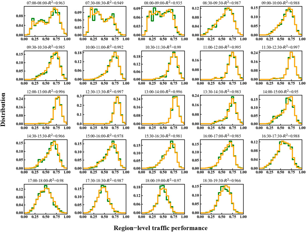
FIGURE A1. Fitting performance of the pairwise maximum entropy model for different time windows. Model fitting performance is evaluated based on its ability to reproduce distribution of macroscopic traffic properties, such as the region-level traffic performance. This performance is defined as the proportion of regions in the largest connected cluster formed by free regions, relative to the total regions. The green curve represents the observed distribution of region-level traffic performance, while the orange curve represents the model-generated distribution. For 24 consecutive one-hour time windows (7:00–18:30, with half-hour sliding intervals), the model achieves a good fitting performance (R²>0.94), successfully capturing both unimodal and bimodal distribution patterns of region-level traffic performance.