A physical state prediction method based on reduce order model and deep learning applied in virtual reality

The application of virtual reality (VR) in industrial training and safety emergency needs to reflect realistic changes in physical object properties. However, existing VR systems still lack fast and accurate simulation of complex, high-fidelity dynamic display of physical object evolution. To enhance the application of VR, a real-time VR visualization method is introduced, which adopts a pre-trained deep learning model to construct high-fidelity physical dynamic changes. This method firstly integrates data dimensionality reduction and temporal convolutional network (TCN) to pre-capture time-series data from numerical simulation results, and then employs Kolmogorov–Arnold Networks (KAN) to approximate nonlinear characteristics to improved Long Short-Term Memory (LSTM) network, thereby predict time-series simulation data accurately to achieves realistic and responsive dynamic displays. The experimental results of predicting time-series numerical simulation data demonstrate that the method balances computational efficiency and achieves good prediction accuracy, with Root Mean Square Error (RMSE) and Mean Absolute Error (MAE) values increased to 0.0087 and 0.0063, respectively. These studies indicate that the proposed method significantly enhances VR’s capability for realistic physical modeling, paving the way for its broader application in high-stakes industrial training and emergency training environments.

1 Introduction

Virtual reality (VR), as a cutting-edge technology, utilizes computer-generated three-dimensional environments to provide an immersive user experience, allowing users to feel a high degree of realism within a virtual space [1]. VR technology is widely applied in various fields such as education, healthcare, and entertainment, enhancing user interaction and offering new possibilities for numerous applications [2–6]. Especially in industrial training secnarios, VR technology integrates physical devices with information systems [7]. Traditional training methods often involve high costs and safety hazards, whereas VR creates a controllable simulation environment, enabling users to practice without jeopardizing themselves or others [8, 9]. Sacks et al. [10] explores the feasibility and effectiveness of using immersive VR technology for architectural safety training, and the authors argue that VR can provide a safe, realistic, and interactive learning environment, thereby improving the learning outcomes and recall ability of participants, ultimately enhancing training effectiveness and worker safety. Liang et al. [11] introduces a serious game based on virtual reality technology designed to enhance safety training efficiency for rock-related hazards in underground mines, and the authors believe that this approach has the potential to improve the safety conditions in underground mines and could be applied to other mining safety training areas, raising miners’ safety awareness and operational skills.

Despite VR’s effectiveness in training has been proven [12], existing VR experiences still show deficiencies in the representation of physical fields [13]. Many VR applications fail to effectively integrate multiple physical fields, such as fluid dynamics and thermodynamics, leading to a reduced sense of immersion and impacting the realistic representation of actual scenarios. This lack of physical field integration not only limits the realism of user experiences but also hinders the promotion of VR technology in complex applications. To address this issue, the combination of VR and physic simulation techniques has gained increasing attention. This integration can dynamically generate more accurate multi-physical fields within VR environments, significantly enhancing the immersive experience for users. The application of these technologies has the potential to drive the further development of VR across various industries, providing new solutions for the simulation of complex systems. However, the methods of physic simulation like Finite Volume Method (FVM) [14] and Finite Element Method (FEM) [15] require significant computational power and time support, which hinders the improvement of efficiency in modeling realistic dynamic scenes in VR, making it difficult to meet the demands for realism and real-time performance [16].

With the advancement of hardware technology, particularly leveraging the parallel processing capabilities of GPUs, neural networks have begun to experience rapid development and large-scale application across various fields [17–20]. For instance, in the realm of time-series prediction, deep learning has provided novel perspectives and methodologies for predicting and simulating non-periodic, complex flows, contrasting with traditional methods that rely on CPU-based computations [21–23]. Deep learning techniques are capable of handling large-scale data and capturing complex non-linear features, making them particularly effective in computational fluid dynamics (CFD) simulations [24, 25]. Guo et al. propose a general and flexible approximation model for real-time prediction of non-uniform steady laminar flow in a 2D or 3D domain based on convolutional neural networks (CNNs) [26]. Kim et al. propose a novel approach that combines CFD simulations with data-driven deep-learning models to predict complex hydrodynamics [27]. Jolaade et al. explore the performance and powerful generative capabilities of both generative adversarial network (GAN) and adversarial autoencoder (AAE) to predict the evolution in time of a highly nonlinear fluid flow [28].

Current challenges in combining deep learning with CFD to build high-fidelity physical fields in VR are listed as follows.

(1) Data Complexity: Deep learning requires capturing both the temporal and spatial characteristics of the data simultaneously. Due to the sequential nature of the problem, deep learning needs continuous input of data to achieve better inference. If the data is too complex, the inference time required is too long and cannot meet the real-time requirements for building high-fidelity physical fields in VR.

(2) Prediction Data Accuracy: Since CFD data is non-linear, deep learning models with strong fitting capabilities are prone to overfitting when the amount of data is insufficient or the model complexity is too high. This can lead to a decline in prediction performance on new data.

In this paper, to address the above-mentioned challenges, a new method for real-time visualization high-fidelity physical fields in VR based on feature pre-capturing method and improved pre-train LSTM is proposed. The specific contributions are described as follows.

(1) An efficient real-time future physical fields construction method is designed, which uses simulation data to pre-train a deep learning model for real-time construction of physical fields based on the current state data in VR.

(2) A module for multi-mixed feature pre-capturing based on data dimensionality reduction is proposed to reduce the dimensionality of the data and capture the current data features to accelerate the inference speed of deep learning.

(3) Utilizing a improve pre-trained model, an effective combination of LSTM and KAN networks is proposed. Leveraging LSTM’s temporal characteristics and KAN’s accuracy in fitting complex functions, the pre-trained model can accurately fit time-series simulation data, thereby establishing a high-fidelity physical field.

This paper employs CFD simulation data of von Karman vortices for experimentation. The experimental results demonstrate that the proposed method effectively balances prediction accuracy and time, achieving optimal prediction results within an allowable time frame, thereby meeting the requirements for the preliminary real-time establishment of high-fidelity physical fields in VR.

The remainder of this study is organized as follows: Section 2 introduce the foundation of this research. The method designed for real-time future physical fields construction is shown in Section 3, which consisting of feature pre-capturing module and improved pre-trained model, while the specific experimental process and results are provided in Section 4. Finally, the conclusions and future works are stated in Section 5.

2 Foundation of proposed methods

2.1 The profile of CFD

Fluid simulation can effectively mimic and predict the behavior of fluids under different conditions, including flow patterns, pressure distributions, and temperature variations [29]. In VR environments, establishing high-fidelity fluid physics fields enhances user immersion, making observation and interaction within the simulation environment more natural, especially in disaster training and high-risk operation training [30–33]. The key formulas in the fluid simulation process are as follows [34, 35]: Continuity Equation: The Continuity Equation describes the principle of conservation of mass in fluids. For incompressible fluids, its formula can be expressed as Equation 1:

$\nabla \cdot \mathbf{u}=0(1)$

where $u$ represents the fluid velocity field.

Momentum Equation (Navier-Stokes Equations): The Navier-Stokes equations describe the conservation of momentum in fluid motion, and its formula is Equation 2:

$\frac{\partial \mathbf{u}}{\partial t}+\left(\mathbf{u}\cdot \nabla \right)\mathbf{u}=-\frac{1}{\rho }\nabla p+\nu {\nabla }^2\mathbf{u}+\mathbf{f}(2)$

where $\rho$ is the fluid density, $p$ is the pressure,$v$ is the kinematic viscosity, and $f$ is the body force (such as gravity).

Energy Equation: The Energy Equation describes the conservation of energy in fluids, typically expressed as Equation 3:

$\frac{\partial E}{\partial t}+\nabla \cdot \left(E\mathbf{u}\right)=-p\nabla \cdot \mathbf{u}+\nabla \cdot \left(\kappa \nabla T\right)+Q(3)$

where $E$ is the total energy per unit volume, $k$ is the thermal conductivity, $T$ is the temperature, and $Q$ is the source term.

The Navier-Stokes equations are fundamental in describing the motion of viscous fluids [36, 37]. They encapsulate the principles of momentum, mass, and energy conservation and can accurately capture the dynamic behavior of fluid flow, such as laminar flow, turbulent flow, and the interaction between fluid and solid boundaries [38, 39]. Consequently, the Navier-Stokes equations are widely applied to various fluid dynamics problems, including gas dynamics, hydrodynamics, climate modeling, and aerospace engineering. They are the cornerstone of fluid simulation in both industrial applications and fundamental research [40].

However, the Navier-Stokes equations are nonlinear, particularly in the convective term $(\mathbf{u}\cdot \nabla )\mathbf{u}$ of the momentum equation [41, 42]. This nonlinearity makes the solution of the equations extremely challenging, especially in complex flow situations such as turbulence, where fluid behavior can become exceedingly intricate [42]. Although the development of modern CFD technology allows engineers and scientists to effectively address these equations using numerical methods, the time and computational resources required are not negligible, particularly in VR scenarios that demand real-time interaction.

2.2 Deep learning applied in physical state prediction

Deep learning models are capable of automatically extracting features from raw data without the need for manual feature engineering [43, 44]. This capability enables the models to better capture complex patterns within the data, particularly excelling in high-dimensional data or nonlinear relationships [45, 46]. They are particularly suitable for handling large-scale datasets, capable of being trained through parallel computing and efficient model structures such as convolutional neural networks and recurrent neural networks. This allows deep learning to maintain good performance as the volume of data continues to increase [47, 48]. For time series data, deep learning can effectively capture temporal dependencies, providing more accurate predictive results [49].

However, there are challenges and difficulties when using deep learning for nonlinear data prediction, especially in the context of AI for science. Training deep learning models on nonlinear data may require complex hyperparameter tuning and substantial computational resources. Particularly when dealing with complex physical phenomena, finding an appropriate network structure and optimization algorithm may necessitate extensive experimentation and iteration. Overfitting is also a particularly prevalent issue. Models may perform well on training data but experience a decline in predictive performance on unseen data. This poses a challenge to the reliability of constructing physical fields in VR, especially when the amount of data is limited.

3 Proposed methods

In this section a real-time physical field prediction method applied in VR is introduced. This novel method contains multi-mixed feature capture and dynamic physical state prediction. The contents of the proposed method will be elaborated in subsequent sections.

3.1 Framework of the proposed method

To present photo-realistic physical state changes, the new method is designed to predict dynamic evolution of virtual object. The framework of the proposed method is shown in Figure 1, which is divided into three core components, namely,: (1) numerical simulation, (2) deep learning model pre-training for data prediction, (3) VR reconstruction. The left side of Figure 1 shows the process of the method, while the right side displays the relevant technologies adopted in each step.

Figure 1

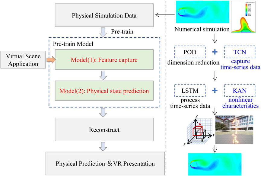
Figure 1. The schematic of the proposed method.

Numerical simulations were conducted using simulation software to obtain simulated physical field data. Simultaneously, a pre-training model was utilized to learn the underlying patterns of physical field variations. Building upon this pre-trained model as the predictive foundation, during VR runtime, the system receives real-time data reflecting changes in the VR environment and predicts future data for reconstruction. The details of the Pre-train Model will be elaborated upon in Sections 3.2 and 3.3.

3.2 Multi-mixed feature pre-capturing module based on data dimensionality reduction

Multi-mixed Feature Pre-capturing module is the module (1) in Figure 1. A set of CFD data is composed of spatial series and time series, where the spatial sequence primarily represents the interrelationship and the overall trend of change between every position within the space at each future time point, while the time series depicts the relationship between the object’s changes at consecutive moments. As the number of parameters that need to be simulated increases, and as the fidelity and duration of the simulation become higher, the volume of data will increase sharply. This will significantly escalate the computational power and time required for deep learning training and inference, even though it already consumes less computational power and time compared to simulations that rely on CPU power [50, 51].

Therefore, this section introduces the Multi-mixed Feature Pre-capturing module proposed in this paper to enhance the effectiveness of deep learning for data prediction, which leverages the advantages of proper orthogonal decomposition (POD) and TCN in feature capturing at different dimensions [52]. Simultaneously, this method perform dimensionality reduction on the data to reduce the computational power and time consumption of deep learning.

(a) POD is applied for data dimensionality reduction due to its effectiveness in capturing the primary flow features. It can simplify the spatial field and generate the temporal field for efficient fluid field reconstruction, where the simplification of the spatial field is shown as Equation 4:

$\left[B,S,V\right]=svd\left(U\right)(4)$

That’s the matrix $U(x,t)=BS{V}^T$, where $B\in R^{M\times M}$, $S\in R^{M\times N}$and $V\in R^{N\times N}$. The set $B$ consists of orthonormal eigenvectors, including the vector ${UU}^T$, and serves as the schema construction matrix for the data. Matrix $S$ is diagonal, with singular values from all solutions arranged in descending order. Vector $V$ represents the spatial mode obtained through decomposition.

The time coefficient is solved with the change of time sequence information of physical field, shown as Equations 5, 6:

$a=B\cdot S(5)$

$\mathbf{a}\left(t\right)={\left[a_1\left(t\right),a_2\left(t\right),\dots ,a_M\left(t\right)\right]}^T(6)$

The time coefficient matrix $\mathbf{a}(t)\in {\mathbb{R}}^{M\times T}$ generated by POD serves as the input to TCN, where $M$ denotes the number of retained modes and $T$ represents the time steps. Reconstruct using obtained parameters, as Equation 7:

$U\left(x,t\right)=\bar{U}\left(x,t\right)+{\displaystyle \sum _{j=1}^p}{a}_j\left(t\right)V_j^T\left(x\right)(7)$

The process described above, by capturing spatial features and analyzing the time matrix, can significantly reduce the amount of data for subsequent processing while retaining important information.

(b) TCN is a deep learning architecture specifically designed for sequence modeling, leveraging convolutional layers to capture temporal dependencies, making it suitable for tasks involving time series data [53]. In this context, to extract short-term features from sequences, TCN employs temporal matrices to capture features along the time dimension. Its uniqueness lies in inserting zero elements between traditional convolution kernels to expand the receptive field, thereby capturing broader temporal features both forwards and backwards without increasing the number of parameters. The TCN formula is described as Equation 8:

${\mathbf{Z}}_{\text{tcn}}=\mathrm{TCN}\left(\mathbf{a}\left(t\right)\right)={\sigma }_{\text{tcn}}\left({\mathbf{W}}_{\text{tcn}}\ast \mathbf{a}\left(t\right)+{\mathbf{b}}_{\text{tcn}}\right)(8)$

where ${\sigma }_{\text{tcn\hspace{0.17em}}}$ denotes the TCN activation function, ${\mathbf{W}}_{tcn}$ represents the convolutional kernel weights, and ${\mathbf{b}}_{\text{tcn}}$ is the bias. The original reconstruction formula $a_j(t)$ is replaced with ${\left[{\mathbf{Z}}_{\text{tcn}}\right]}_j$, which represents the time coefficients optimized by TCN, while retaining the POD spatial basis $V_j(x)$. The formula is Equation 9:

$U\left(x,t\right)=\bar{U}\left(x,t\right)+{\displaystyle \sum _{j=1}^p}{\left[{\mathbf{Z}}_{\text{tcn}}\right]}_j{V}_j^T\left(x\right)(9)$

TCN and POD are combined to capture features, based on their sensitivity in terms of space and time. The framework is shown as in Figure 2. The TCN is used as the next step after the decomposition of the time and space matrices in the POD process, further capturing the temporal features of the time matrix to serve as preprocessed data ready for the subsequent data prediction step.

Figure 2

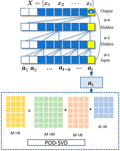
Figure 2. Feature pre-capture module.

3.3 Prediction module based on improved pre-train LSTM

Prediction module is the module (2) in Figure 1, and the structure is shown in Figure 3. Directly using simulations to establish future physical fields in real-time may place stringent demands on computational power. Therefore, employing a pre-trained deep learning module to construct physical fields is considered as one of the options. LSTM networks, due to their unique gating mechanism, exhibit significant advantages in processing time-series data [54]. Meanwhile, pre-trained models based on LSTM networks hold great potential in addressing the instantaneity issues of VR presentation and the temporal problems of physical simulation data prediction.

Figure 3

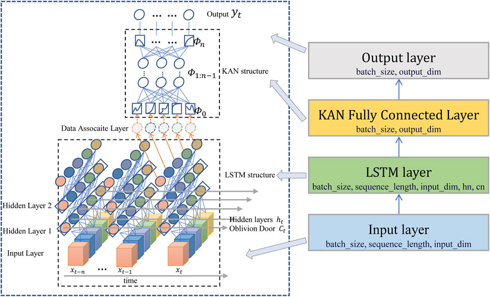
Figure 3. Improved pre-train LSTM.

The LSTM unit is comprised of three parts: the forget gate, the input gate, and the output gate. The forget gate determines how much information from the previous time step’s cell state is retained, the input gate controls how much input information is added at the current time step, and the output gate decides how much information is output from the current cell state. The computational formulas for the LSTM unit are as follows Equations 10–15:

$f_t=\sigma \left(W_f\cdot \left[h_{t-1},x_t\right]+b_f\right)(10)$

$i_t=\sigma \left(W_i\cdot \left[h_{t-1},x_t\right]+b_i\right)(11)$

${\tilde{C}}_t=\tanh \left(W_C\cdot \left[h_{t-1},x_t\right]+b_C\right)(12)$

$C_t=f_t\ast C_{t-1}+i_t\ast {\tilde{C}}_t(13)$

$o_t=\sigma \left(W_o\left[h_{t-1},x_t\right]+b_o\right)(14)$

$h_t=o_t\ast \tanh \left(C_t\right)(15)$

In this context, $f_t$, $i_t$, $o_t$, and ${\tilde{C}}_t$ stand for the forget gate, input gate, output gate, and candidate vector, respectively. $W_f$, $W_i$, $W_C$, and another $W_o$ represent weight matrices. $b_f$, $b_i$, $b_C$, and $b_o$ represent bias vectors. sigma and $tanh$ denote the sigmoid and hyperbolic tangent functions, respectively, $c$ represents the cell state.

However, despite LSTM’s excellent performance in handling short to medium-length time-series data, its performance is often limited when faced with long, nonlinear time-series data. This is due to the presence of nonlinear convective terms in the Navier-Stokes equations, whereas the traditional fully connected layers within LSTM algorithms, equipped with fixed activation functions, possess limited fitting capabilities for such nonlinearity. Consequently, we adopted the KAN network. The KAN leverage learnable activation functions, enabling them to approximate arbitrary continuous functions, which makes them particularly well-suited for highly nonlinear CFD data. Furthermore, KAN permit the incorporation of domain knowledge—for example, initializing the network with spline bases—ensuring that the outputs adhere to the conservation laws of fluid dynamics. The Kolmogorov-Arnold Representation Theorem serves as the theoretical foundation for KAN networks. This theorem states that any multivariate continuous function $f(x_1,x_2,\dots ,x_n)$ can be represented as a composition of a finite number of univariate continuous functions ${\mathrm{\Phi }}_{q,p}$ and binary addition operations, where both ${\mathrm{\Phi }}_q$ and ${\phi }_{q,p}$ are univariate continuous functions. the theorem can be formulated as Equation 16:

$f\left(x_1,x_2,\dots ,x_n\right)={\displaystyle \sum _{q-1}^{2n+1}}{\mathrm{\Phi }}_q\left({\displaystyle \sum _{p-1}^n}{\phi }_{q,p}\left(x_p\right)\right)(16)$

As input data passes through a KAN layer, it first undergoes computation with these learnable activation functions to obtain output values. These learnable activation functions are positioned on the edges of the network, rather than on the neurons. Mathematically, this process can be expressed as Equation 17:

$x^{\left(l+1\right)}={\sigma }^{\left(l+1\right)}\left(W^{\left(l+1\right)}\cdot {\sigma }^{\left(l\right)}\left(x^{\left(l\right)}\right)\right)(17)$

${\sigma }^{(l)}$ and ${\sigma }^{(l+1)}$ denote the adjustable radial basis functions for the lth and $(l+1)$-th layers, respectively. Various complex functions can often be approximated by a relatively small number of radial basis functions. Here, $w$ represents the weight matrix, $x^{(l)}$ and $x^{(l+1)}$ denotes the input and output. The total training loss is the sum of the prediction loss and the L1 and entropy regularization terms for all KAN layers, as Equation 18:

${\ell }_{\text{total\hspace{0.17em}}}={\ell }_{\text{pred\hspace{0.17em}}}+\lambda \left({\mu }_1{\displaystyle \sum _{l=0}^{L-1}}{\left|{\mathbf{\Phi }}_l\right|}_1+{\mu }_2{\displaystyle \sum _{l=0}^{L-1}}S\left({\mathbf{\Phi }}_l\right)\right)(18)$

${\left|{\mathbf{\Phi }}_l\right|}_1$ represents the sum of the L1 norms of all activation functions for each layer, while $S\left({\mathbf{\Phi }}_l\right)$ represents the entropy for each layer. Unlike previous LSTM network predictions, replacing the last fully connected layer of the LSTM network with a KAN network containing a conditionally parameterized function layer enables the activation functions to become learnable without increasing the number of parameters. If take the output at the final time step of the LSTM network, denoted as $ylstm$, as the input to the KAN, then the output of the KAN network is as follow Equation 19:

${\widehat{y}}_{KAN}={\sigma }^{\left(L\right)}\left(W^{\left(L\right)}{\sigma }^{\left(L-1\right)}\left(W^{\left(L-1\right)}\cdots {\sigma }^{\left(1\right)}\left(W^{\left(1\right)}{\widehat{y}}_{LSTM,L}+{\mathbf{b}}^{\left(1\right)}\right)\cdots +{\mathbf{b}}^{\left(L-1\right)}\right)+{\mathbf{b}}^{\left(L\right)}\right)(19)$

The activation functions for the KAN layers can be directly set by individuals, after which affine functions can be fit. The injection of human inductive biases or domain knowledge allows for more accurate fitting results.

Therefore, in this subsection, a method is proposed that leverages the strengths of LSTM and KAN to pre-train a deep learning module using simulation data, thereby enabling real-time responses to changes in physical states within VR.

4 Validation

4.1 Dataset and experimental environments

The data on which this paper adopted can be found in [http://dmdbook.com/]. The paper utilizes the 2D flow around a circular cylinder with von Kármán vortices in the dataset to demonstrate and validate the method proposed in this paper. All the experiments are implemented on the platform Python and on a work station with Intel i7, GPU 4060 and Windows 11. The high realistic dynamic presentation of fluid dynamics is a common need in virtual reality scenes. This section applies the proposed method of a deep learning prediction based on CFD simulation to achieve fast generation of highly realistic animations. The phenomenon of von Kármán vortices is a typical scenario in numerical simulation of fluid dynamics, and the CFD simulation data in this paper comes from the above dataset, the Reynolds number is 100, with a time interval of 0.02s and 150 data snapshots taken at various time points. The Strouhal number is 0.16, and the simulation domain is divided into 199 grids along the x-direction and 449 grids along the y-direction.

4.2 Experiments and analysis

In the simulation analysis, we focused on the temporal evolution of fluid dynamics. Figure 4 presents the evolution at two time points, t1 = 2 s and t2 = 3.02 s. Figure 5 displays a schematic diagram that visually represents the sixth-order mode within the flow field.

Figure 4

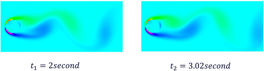
Figure 4. Cylindrical flow field with 89,351 nodes.

Figure 5

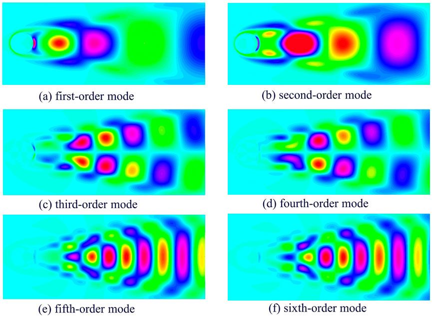
Figure 5. The main POD mode distribution in flow field.

Among all linear combinations, the one corresponding to POD is superior in that it captures the most kinetic energy on average. The energy relationship between time and space fields is quantified using Equation 20, which establishes that the cumulative energy of the first $N_k$ modes in the reduced space is always greater than or equal to the cumulative energy of the corresponding modes in the original space. This inequality holds for every $N_k\le N$, ensuring that the dominant modes capture the essential dynamics of the system with minimal energy loss [55]. Based on the energy ranking shown in Figure 6, it is evident that the energies of the first six orders suffice to approximate the reduced flow field [56]. Therefore, the time coefficient data of these six modes are selected as the training dataset. The comparative analysis seeks to elucidate the influence of various modal data on the model’s predictive capabilities.

${\displaystyle \sum _{i=1}^{N_k}}E\left\{{\beta }_i{\beta }_i\right\}={\displaystyle \sum _{i=1}^{N_k}}{\lambda }_i⩾{\displaystyle \sum _{i=1}^{N_k}}E\left\{{\alpha }_i{\alpha }_i\right\},\text{\hspace{0.17em}for\hspace{0.17em}every\hspace{0.17em}}{N}_k⩽N(20)$

Figure 6

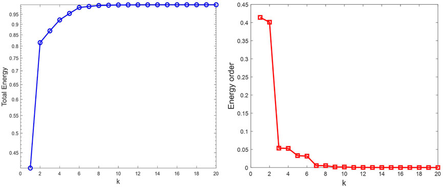
Figure 6. The magnitude of modal energy at different modes.

In the experiments conducted in this paper, multiple parameters were employed to configure the neural network model. Initially, the batch size was set to 10. To facilitate the processing of multi-dimensional data, an extra dimension L with a value of three was introduced. The input layer consists of 50 neurons, tasked with receiving the raw data features. The hidden layer was expanded to 200 neurons, enhancing the model’s nonlinear representation capability and capacity. The output layer comprises 100 neurons. Additionally, a task-specific parameter, gridsize, was defined with a value of 300, which determines the size of the grid search. The model was trained for 500 epochs, and the learning rate of the Adam optimizer was set to 5e-4. To improve the model’s learning efficiency and stability, normalization was applied to the input data, unifying the data scale to the same magnitude and accelerating the convergence process. For the output layer, the tanh function was chosen as the activation function, capable of producing outputs within the range of −1 to 1, thereby enhancing the model’s flexibility and effectiveness in tasks requiring bounded output ranges. Throughout the design of the convolutional layers, the ReLU function was uniformly adopted as the activation function. The KAN layer is configured with: grid size = 5; spline order = 3; noise scaling = 0.1; base scaling = 1.0; spline scaling = 1.0; grid range [-1, 1]; grid smoothing = 0.02. Training employs a composite loss function, as Equation 21:

${\ell }_{\text{total}}=\frac{1}{T}{\displaystyle \sum _{t=1}^T}{‖{\mathbf{y}}_t-{\widehat{\mathbf{y}}}_t‖}_{\mathrm{\Gamma }}^2+\lambda \left({\mu }_1{\displaystyle \sum _{l=0}^{L-1}}{\left|{\mathbf{\Phi }}_l\right|}_1+{\mu }_2{\displaystyle \sum _{l=0}^{L-1}}S\left({\mathbf{\Phi }}_l\right)\right)(21)$

Additionally, $\mathrm{\Gamma }$ is the vorticity-related weight matrix the regularization coefficient is set to $\lambda =0.01,{\mu }_1=0.1,{\mu }_2=0.05$, and a Dropout layer is added with a ratio of 0.2, along with an early stopping strategy with a patience of 20. The dataset comprises time coefficients for six initial patterns across 225 time steps, with the simulation process lasting 6.04 s. To ensure prediction accuracy, a multi-input single-output model was employed. For model evaluation, R²; was selected as the assessment metric. Figures 7–10 show the predictive performance of four commonly used networks, while Figure 11 illustrates the predictive performance of the proposed method in this paper to evaluate its predictive capability.

Figure 7

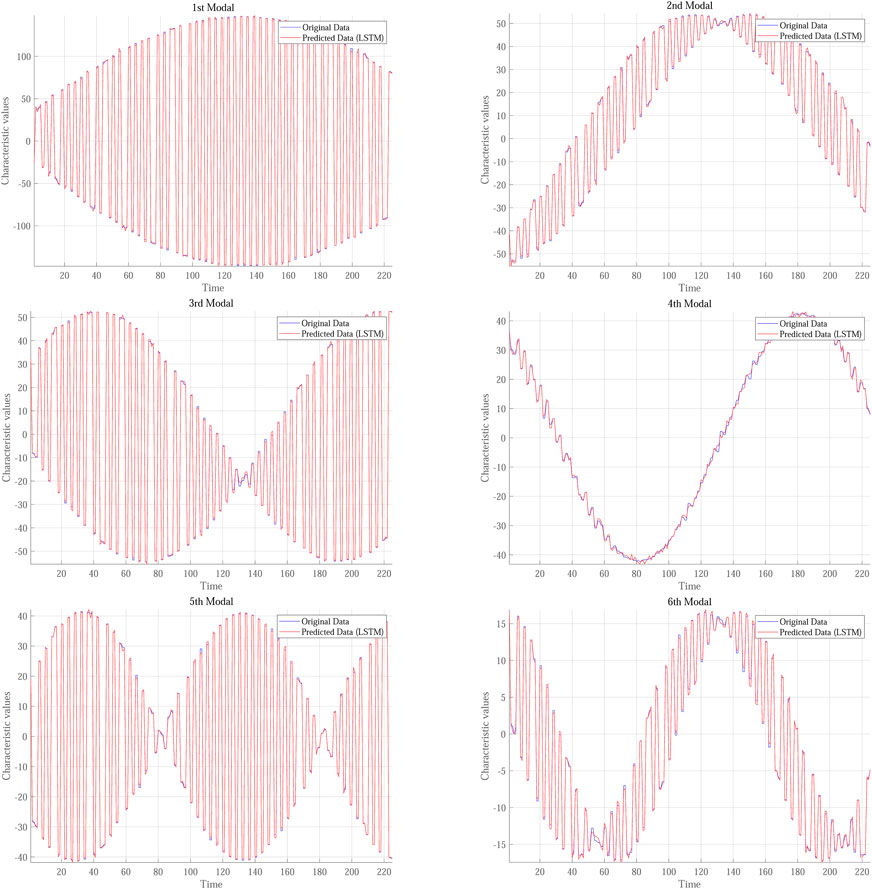
Figure 7. The predicted data of LSTM compared with original data.

Figure 8

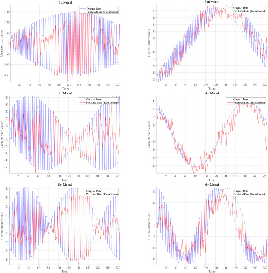
Figure 8. The predicted data of Transformer compared with original data.

Figure 9

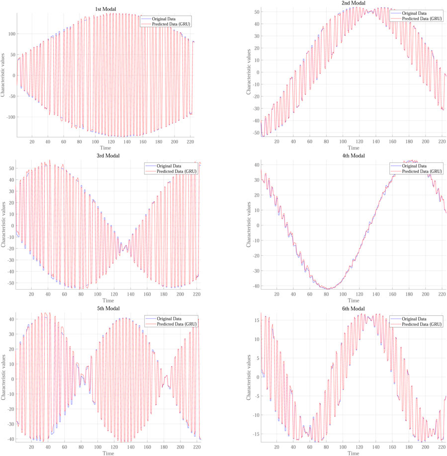
Figure 9. The predicted data of GRU compared with original data.

Figure 10

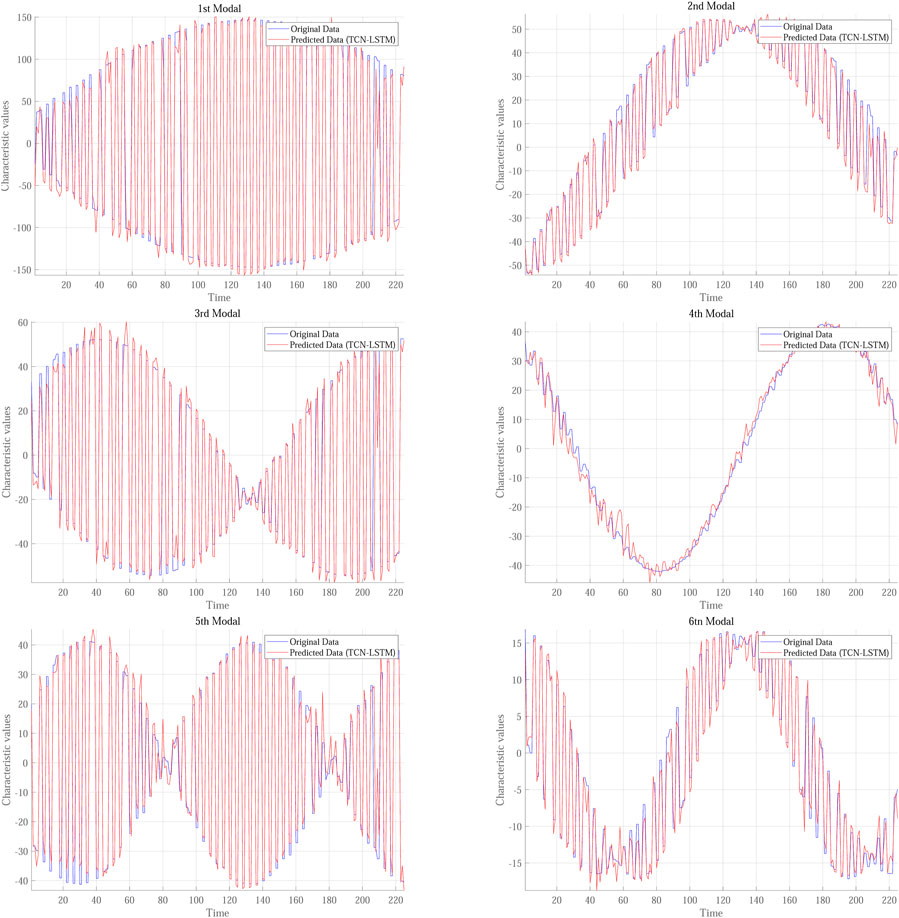
Figure 10. The predicted data of TCN-LSTM compared with original data.

Figure 11

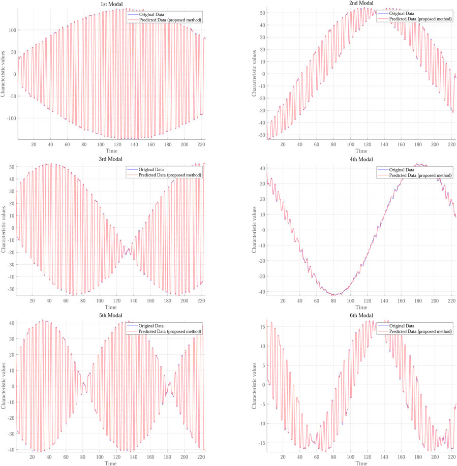
Figure 11. The predicted data of proposed method compared with original data.

As shown in Figure 12, the method proposed in this paper exhibits extremely high stability during the training process when compared to the unmodified model. The R² value rapidly increases from the initial stage to nearly one and remains at this high level throughout the subsequent training, with fluctuations but overall demonstrating very stable performance. This indicates that the model is capable of fitting the data exceptionally well, with prediction results closely aligning with actual values, thereby demonstrating its powerful predictive capabilities.

Figure 12

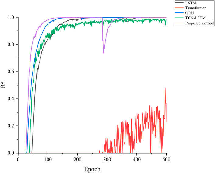
Figure 12. The R² value of different methods.

Table 1 compares the time consumption and Root Mean Square Error (RMSE) of different models, all of which utilize data from the first six modes as both input and output. As indicated in the table, the Transformer model operates the slowest and exhibits significantly poorer prediction accuracy, suggesting that further optimization and stabilization may be necessary. The GRU model consumes even more time, posing potential challenges when faced with real-time requirements. In contrast, the model proposed based on feature pre-capture compares favorably in computation time with the LSTM and TCN-LSTM models. However, in terms of performance, the model proposed based on feature pre-capture outperforms the other methods.

Table 1

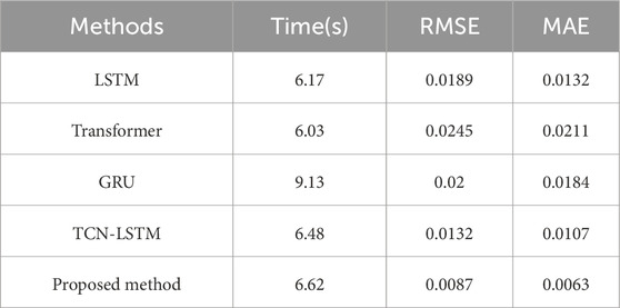
Table 1. The time consumption of different models in the sixth-order mode is compared with that of RMSE and MAE.

To present the prediction results more intuitively, Three different time points were selected, and a sixth-order improved LSTM model network based on feature pre-capture was employed to compare the actual and predicted scenarios at these time points. The prediction model accurately forecasted the data features or states at the 1-s, 3-s, and 5-s marks, with high confidence levels in the prediction results, that shown in Figure 13. This demonstrates that, in situations where future simulation data is unavailable, the prediction model can effectively predict the physical field in a reduced-order model state, showcasing its robust prediction capabilities and practical application value.

Figure 13

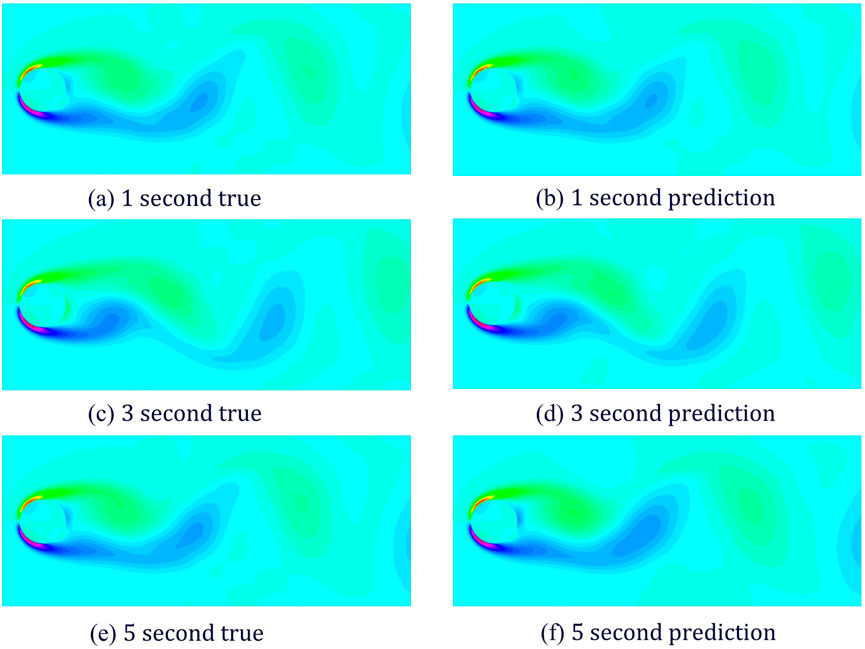
Figure 13. Comparison of real and predicted effects of the six-order modal reconstructed flow field under 1, 3, and 5 s time coefficient predictions of the improved model.

Ultimately, with the reduction to the first six modes, the original flow field is propelled forward by twenty time steps, attaining a duration of 6.44 s (Figure 14). Regardless of whether the transmission into virtual reality is data-driven or dynamic, the resultant effects will invariably encapsulate physical properties.

Figure 14

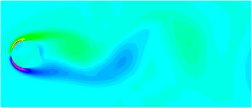
Figure 14. Based on the time coefficient prediction of the improved model, the future state of the flow field at 6.44 s is obtained.

4.3 Application and prospects of the proposed methods

The physical state prediction method proposed in this paper will be applied to the presentation of VR realistic dynamic scenes. Taking the animation presentation of ice droplet melting in the simulation training of civil aviation aircraft de icing as an example. The application diagram is shown in Figure 15. Using the method proposed in this paper, numerical simulation analysis is conducted during the initial stage of the melting process of frozen droplets, followed by data-driven prediction to obtain the physical property changes of the melting process. This method can significantly shorten the time required to obtain the variation pattern of the simulated object using only multi physics field coupled numerical simulation. In VR scenes, the changing patterns of the melting process of frozen droplets are associated with the particle system in the form of structured data. By simulating the generation, attribute changes, and disappearance process of particles through the particle system, a dynamic effect of melting is constructed. The VR visual effects enhanced by this method integrate the real laws of physical property changes, and can present realistic animation effects. This study conducts training on laminar flow at Re = 100, while the strong nonlinear dynamics of high-Reynolds-number turbulence have not been investigated. Future work will explore adaptive modal selection mechanisms and differentiable rendering techniques to balance the accuracy of complex flow regimes with the deployment efficiency on edge devices.

Figure 15

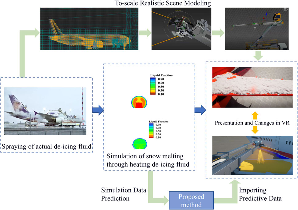
Figure 15. Application of physical state prediction methods in VR aircraft ice removal.

5 Conclusion and future works

This paper proposed an effective method for real-time construction of future physical fields within the VR environment. This is achieved via rapid prediction of high-fidelity physical fields integrated multi-mixed feature pre-capturing module based on data dimensionality reduction and prediction module based on improved pre-train LSTM. Owing to these two modules, the characteristics of the simulated data can be effectively fitted, allowing for the timely prediction of high-fidelity future physical fields based on the current state during VR usage, and the real-time establishment of these physical fields within the VR environment.

The numerical results indicate that, compared to the computation time of traditional CFD simulations, the prediction model introduced in this paper offers at least a 160-fold reduction in computation time. Furthermore, compared to existing deep learning methods, the proposed method effectively balances prediction accuracy and time consumption, thereby essentially meeting the requirements for real-time presentation in VR environments.

However, the method proposed in this paper experiences an exponential reduction in the number of data points for temporal coefficients during the data reduction process. This may result in an inability to meet the data requirements of deep learning networks when dealing with specific issues. Additionally, this study focuses solely on training for laminar flow at a Reynolds number (Re) of 100. The strong nonlinear dynamics associated with high Reynolds number turbulent flows (Re $>$ 1,000) have not been investigated. Future work will explore adaptive mode selection mechanisms, differentiable rendering techniques, and reducing algorithmic complexity, aiming to balance the accuracy required for complex flow regimes with the efficiency of deployment on edge devices.

Data availability statement

Publicly available datasets were analyzed in this study. This data can be found here: The data on which this paper adopted can be found in [http://dmdbook.com/].

Author contributions

PY: Writing – original draft. QL: Writing – original draft. SY: Writing – review and editing, Investigation. MZ: Writing – review and editing, Writing – original draft. YH: Writing – original draft. GZ: Writing – review and editing.

Funding

The author(s) declare that financial support was received for the research and/or publication of this article. This work was supported by the Science and Technology Program of Sichuan Province (2024YFHZ0020); The Key Research and Development Projects of Sichuan-Chongqing Alliance (CSTB2022TIAD-CUX0018); Research Foundation of Chengdu University of Information Technology (KYTZ2023009).

Conflict of interest

Author QL was employed as postdoctoral researcher by Chongqing Saibao Industrial Technology Research Institute Co., Ltd.

The remaining authors declare that the research was conducted in the absence of any commercial or financial relationships that could be construed as a potential conflict of interest.

Generative AI statement

The author(s) declare that no Generative AI was used in the creation of this manuscript.

Publisher’s note

All claims expressed in this article are solely those of the authors and do not necessarily represent those of their affiliated organizations, or those of the publisher, the editors and the reviewers. Any product that may be evaluated in this article, or claim that may be made by its manufacturer, is not guaranteed or endorsed by the publisher.

References

1. Frederick PB. What’s real about virtual reality? IEEE Computer graphics Appl (1999) 19(6):16–27. doi:10.1109/38.799723

CrossRef Full Text | Google Scholar

2. Jerald J. The VR book: human-centered design for virtual reality. San Rafael: Morgan & Claypool (2015).

Google Scholar

3. Zhang Y, Liu H, Kang S-C, Al-Hussein M. Virtual reality applications for the built environment: research trends and opportunities. Automation in Construction (2020) 118:103311. doi:10.1016/j.autcon.2020.103311

CrossRef Full Text | Google Scholar

4. Lee J-K, Lee S, Kim Y-chae, Kim S, Hong S-W. Augmented virtual reality and 360 spatial visualization for supporting user-engaged design. J Comput Des Eng (2023) 10(3):1047–59. doi:10.1093/jcde/qwad035

CrossRef Full Text | Google Scholar

5. Liagkou V, Salmas D, Stylios C. Realizing virtual reality learning environment for industry 4.0. Proced Cirp (2019) 79:712–7. doi:10.1016/j.procir.2019.02.025

CrossRef Full Text | Google Scholar

6. Rehman IU, Ullah S, Ali N, Rabbi I, Ullah Khan R. Gesture-based guidance for navigation in virtual environments. J Multimodal User Inter (2022) 16(4):371–83. doi:10.1007/s12193-022-00395-1

CrossRef Full Text | Google Scholar

7. Huang Y, Lu X. Editorial: security, governance, and challenges of the new generation of cyber-physical-social systems. Front Phys (2024) 12(1464919). doi:10.3389/fphy.2024.1464919

CrossRef Full Text | Google Scholar

8. Tan Y, Xu W, Li S, Chen K. Augmented and virtual reality (ar/vr) for education and training in the aec industry: a systematic review of research and applications. Buildings (2022) 12(10):1529. doi:10.3390/buildings12101529

CrossRef Full Text | Google Scholar

9. Feng Z, González VA, Amor R, Lovreglio R, Cabrera-Guerrero G. Immersive virtual reality serious games for evacuation training and research: a systematic literature review. Comput and Education (2018) 127:252–66. doi:10.1016/j.compedu.2018.09.002

CrossRef Full Text | Google Scholar

10. Sacks R, Perlman A, Barak R. Construction safety training using immersive virtual reality. Construction Management Econ (2013) 31(9):1005–17. doi:10.1080/01446193.2013.828844

CrossRef Full Text | Google Scholar

11. Liang Z, Zhou K, Gao K. Development of virtual reality serious game for underground rock-related hazards safety training. IEEE access (2019) 7:118639–49. doi:10.1109/access.2019.2934990

CrossRef Full Text | Google Scholar

12. Stefan H, Mortimer M, Horan B. Evaluating the effectiveness of virtual reality for safety-relevant training: a systematic review. Virtual Reality (2023) 27(4):2839–69. doi:10.1007/s10055-023-00843-7

CrossRef Full Text | Google Scholar

13. Li Z, Liu H, Dai R, Su X. Application of numerical analysis principles and key technology for high fidelity simulation to 3-d physical model tests for underground caverns. Tunnelling Underground Space Technology (2005) 20(4):390–9. doi:10.1016/j.tust.2005.01.004

CrossRef Full Text | Google Scholar

14. Moukalled F, Mangani L, Darwish M, Moukalled F, Mangani L, Darwish M. The finite volume method. Springer (2016).

Google Scholar

15. Jagota V, Sethi APS, Kumar K. Finite element method: an overview. Walailak J Sci Technology (Wjst) (2013) 10(1):1–8. doi:10.2004/wjst.v10i1.499

CrossRef Full Text | Google Scholar

16. Jayaram S, Vance J, Gadh R, Jayaram U, Srinivasan H. Assessment of vr technology and its applications to engineering problems. J Comput Inf Sci Eng (2001) 1(1):72–83. doi:10.1115/1.1353846

CrossRef Full Text | Google Scholar

17. Khan RU, Almakdi S, Alshehri M, Haq AU, Ullah A, Kumar R. An intelligent neural network model to detect red blood cells for various blood structure classification in microscopic medical images. Heliyon (2024) 10(4):e26149. doi:10.1016/j.heliyon.2024.e26149

PubMed Abstract | CrossRef Full Text | Google Scholar

18. Liu Q, Wang K, Li Y, Liu Y. Data-driven concept network for inspiring designers’ idea generation. J Comput Inf Sci Eng (2020) 20(3):031004. doi:10.1115/1.4046207

CrossRef Full Text | Google Scholar

19. Liu Q, Wang K, Li Y, Chen C, Li W. A novel function-structure concept network construction and analysis method for a smart product design system. Adv Eng Inform (2022) 51:101502. doi:10.1016/j.aei.2021.101502

CrossRef Full Text | Google Scholar

20. Hu Y, Wu Y, Yang Q, Liu Y, Wang S, Dong J, et al. An approach for detecting faulty lines in a small-current, grounded system using learning spiking neural p systems with nlms. Energies (19961073) (2024) 17(22):5742. doi:10.3390/en17225742

CrossRef Full Text | Google Scholar

21. Pant P, Doshi R, Bahl P, Farimani AB. Deep learning for reduced order modelling and efficient temporal evolution of fluid simulations. Phys Fluids (2021) 33(10):2021. doi:10.1063/5.0062546

CrossRef Full Text | Google Scholar

22. Khan RU, Almakdi S, Alshehri M, Kumar R, Ali I, Hussain SM, et al. Probabilistic approach to covid-19 data analysis and forecasting future outbreaks using a multi-layer perceptron neural network. Diagnostics (2022) 12(10):2539. doi:10.3390/diagnostics12102539

PubMed Abstract | CrossRef Full Text | Google Scholar

23. Khan RU, Kumar R, Haq AU, Khan I, Shabaz M, Khan F. Blockchain-based trusted tracking smart sensing network to prevent the spread of infectious diseases. IRBM (2024) 45(2):100829. doi:10.1016/j.irbm.2024.100829

CrossRef Full Text | Google Scholar

24. Nathan Kutz J. Deep learning in fluid dynamics. J Fluid Mech (2017) 814:1–4. doi:10.1017/jfm.2016.803

CrossRef Full Text | Google Scholar

25. Brunton SL, Noack BR, Koumoutsakos P. Machine learning for fluid mechanics. Annu Rev Fluid Mech (2020) 52(1):477–508. doi:10.1146/annurev-fluid-010719-060214

CrossRef Full Text | Google Scholar

26. Guo X, Li W, Iorio F. Convolutional neural networks for steady flow approximation. In: Proceedings of the 22nd ACM SIGKDD international conference on knowledge discovery and data mining (2016). p. 481–90.

Google Scholar

27. Kim H, Park M, Kim CW, Shin D. Source localization for hazardous material release in an outdoor chemical plant via a combination of lstm-rnn and cfd simulation. Comput and Chem Eng (2019) 125:476–89. doi:10.1016/j.compchemeng.2019.03.012

CrossRef Full Text | Google Scholar

28. Jolaade M, Silva VLS, Heaney CE, Pain CC. Generative networks applied to model fluid flows. In: International conference on computational science. Springer (2022). p. 742–55.

Google Scholar

29. Zhao Z, Zhou L, Bai L, Wang B, Agarwal R. Recent advances and perspectives of cfd–dem simulation in fluidized bed. Arch Comput Methods Eng (2024) 31(2):871–918. doi:10.1007/s11831-023-10001-6

CrossRef Full Text | Google Scholar

30. Wang M, Ju H, Wu J, Qiu H, Liu K, Tian W, et al. A review of cfd studies on thermal hydraulic analysis of coolant flow through fuel rod bundles in nuclear reactor. Prog Nucl Energy (2024) 171:105175. doi:10.1016/j.pnucene.2024.105175

CrossRef Full Text | Google Scholar

31. Mishra KB. Cfd model for large hazardous dense cloud spread predictions, with particular reference to bhopal disaster. Atmos Environ (2015) 117:74–91. doi:10.1016/j.atmosenv.2015.06.038

CrossRef Full Text | Google Scholar

32. Li Q, Zhou S, Wang Z. Quantitative risk assessment of explosion rescue by integrating cfd modeling with grnn. Process Saf Environ Prot (2021) 154:291–305. doi:10.1016/j.psep.2021.08.029

CrossRef Full Text | Google Scholar

33. Li S, Bu L, Shi S, Li L, Zhou Z. Prediction for water inrush disaster source and cfd-based design of evacuation routes in karst tunnel. Int J Geomechanics (2022) 22(5):05022001. doi:10.1061/(asce)gm.1943-5622.0002305

CrossRef Full Text | Google Scholar

34. Ferziger JH, Perić M, Street RL. Computational methods for fluid dynamics. New York: Springer (2019).

Google Scholar

35. Grabe M. Measurement uncertainties in science and technology. Springer (2014).

Google Scholar

36. Constantin P, Foiaş C. Navier-Stokes equations. University of Chicago press (1988).

Google Scholar

37. Joel Chorin A. Numerical solution of the Navier-Stokes equations. Mathematics Comput (1968) 22(104):745–62. doi:10.1090/s0025-5718-1968-0242392-2

CrossRef Full Text | Google Scholar

38. Doering CR, Gibbon JD. Applied analysis of the Navier-Stokes equations. Cambridge: Cambridge University Press (1995).

Google Scholar

39. Foias C, Manley O, Rosa R, Temam R Navier-Stokes equations and turbulence, 83. Cambridge University Press (2001).

Google Scholar

40. Horgan CO, Wheeler LT. Spatial decay estimates for the Navier–Stokes equations with application to the problem of entry flow. SIAM J Appl Mathematics (1978) 35(1):97–116. doi:10.1137/0135008

CrossRef Full Text | Google Scholar

41. Marion M, Temam R. Navier-Stokes equations: theory and approximation. Handbook Numer Anal (1998) 6:503–689. doi:10.1016/s1570-8659(98)80010-0

CrossRef Full Text | Google Scholar

42. Temam R. Navier–Stokes equations and nonlinear functional analysis. Philadelphia: Society for Industrial and Applied Mathematics (1995).

Google Scholar

43. Emmert-Streib F, Yang Z, Feng H, Tripathi S, Dehmer M. An introductory review of deep learning for prediction models with big data. Front Artif Intelligence (2020) 3(4):4. doi:10.3389/frai.2020.00004

PubMed Abstract | CrossRef Full Text | Google Scholar

44. Lv Y, Duan Y, Kang W, Li Z, Wang F-Y. Traffic flow prediction with big data: a deep learning approach. Ieee Trans Intell transportation Syst (2014) 16(2):865–73. doi:10.1109/TITS.2014.2345663

CrossRef Full Text | Google Scholar

45. Herrmann L, Kollmannsberger S. Deep learning in computational mechanics: a review. Comput Mech (2024) 74(2):281–331. doi:10.1007/s00466-023-02434-4

CrossRef Full Text | Google Scholar

46. Liu J, Zhang T, Sun S. Review of deep learning algorithms in molecular simulations and perspective applications on petroleum engineering. Geosci Front (2024) 15:101735. doi:10.1016/j.gsf.2023.101735

CrossRef Full Text | Google Scholar

47. Kim J, Kim H, Kim HG, Lee D, Yoon S. A comprehensive survey of deep learning for time series forecasting: architectural diversity and open challenges. Artif Intelligence Rev (2025) 58(7):216–95. doi:10.1007/s10462-025-11223-9

CrossRef Full Text | Google Scholar

48. Mohammadi Foumani N, Miller L, Tan CW, Webb GI, Forestier G, Salehi M. Deep learning for time series classification and extrinsic regression: a current survey. ACM Comput Surv (2024) 56(9):1–45. doi:10.1145/3649448

CrossRef Full Text | Google Scholar

49. Han Z, Zhao J, Leung H, Ma KF, Wang W. A review of deep learning models for time series prediction. IEEE Sensors J (2019) 21(6):7833–48. doi:10.1109/jsen.2019.2923982

CrossRef Full Text | Google Scholar

50. Lucia DJ, Beran PS, Silva WA. Reduced-order modeling: new approaches for computational physics. Prog aerospace Sci (2004) 40(1-2):51–117. doi:10.1016/j.paerosci.2003.12.001

CrossRef Full Text | Google Scholar

51. Lassila T, Manzoni A, Quarteroni A, Rozza G. Model order reduction in fluid dynamics: challenges and perspectives. In: Reduced Order Methods for modeling and computational reduction (2014). p. 235–73.

Google Scholar

52. Huang Y, Yu J, Wang D, Lu X, Dufaux F, Guo H, et al. Learning-based fast splitting and directional mode decision for vvc intra prediction. IEEE Trans Broadcasting (2024) 70(2):681–92. doi:10.1109/tbc.2024.3360729

CrossRef Full Text | Google Scholar

53. Hewage P, Behera A, Trovati M, Pereira E, Ghahremani M, Palmieri F, et al. Temporal convolutional neural (tcn) network for an effective weather forecasting using time-series data from the local weather station. Soft Comput (2020) 24:16453–82. doi:10.1007/s00500-020-04954-0

CrossRef Full Text | Google Scholar

54. Yu Y, Si X, Hu C, Zhang J. A review of recurrent neural networks: lstm cells and network architectures. Neural Comput (2019) 31(7):1235–70. doi:10.1162/neco_a_01199

PubMed Abstract | CrossRef Full Text | Google Scholar

55. Ravindran SS. Reduced-order adaptive controllers for fluid flows using pod. J scientific Comput (2000) 15:457–78. doi:10.1023/a:1011184714898

CrossRef Full Text | Google Scholar

56. Azam SE, Mariani S. Investigation of computational and accuracy issues in pod-based reduced order modeling of dynamic structural systems. Eng structures (2013) 54:150–67. doi:10.1016/j.engstruct.2013.04.004

CrossRef Full Text | Google Scholar