Dynamic risk prediction in financial-production systems using temporal self-attention and adaptive autoregressive models

In financial production systems, accurate risk prediction is crucial for decision- makers. Traditional forecasting methods face certain limitations when dealing with complex time-series data and nonlinear dependencies between systems, especially under extreme market fluctuations. To address this, we propose an innovative hybrid temporal model, TSA-AR (Temporal Self-Attention Adaptive Autoregression), which combines temporal self-attention mechanisms with an adaptive autoregressive model to solve the risk prediction problem in financial and production systems. TSA-AR performs multi-scale feature extraction through an improved Informer encoder, dynamically adjusts model parameters with a dynamic autoregressive module, and constructs the nonlinear dependencies between financial and production systems through a cross_modal interaction graph. Experimental results show that TSA-AR achieves an MSE of 0.0689, significantly lower than other comparative models (e.g., Transformer’s 0.0921), and performs excellently with an Extreme Risk Detection Rate of 81.70%. The model effectively improves the accuracy and stability of risk prediction, providing a more accurate forecasting tool for financial-production system risk management, with significant practical implications.

1 Introduction

In recent years, the coupling between global financial systems and real-world production systems has intensified, leading to the formation of a complex risk transmission network. Studies have shown that financial market fluctuations can quickly transmit to the real economy through mechanisms such as credit channels and investment contraction [1, 2]. Conversely, disruptions in production systems (e.g., supply chain breakdowns, insufficient capacity) can have a feedback effect on financial markets, creating a negative feedback loop [3, 4]. For instance, during the COVID-19 pandemic in 2020, a liquidity crisis in the financial markets led to a surge in corporate financing costs, which subsequently triggered widespread delays in global supply chains [5–7]. Similarly, in 2022, the Federal Reserve’s aggressive interest rate hikes not only caused stock market turbulence but also suppressed fixed asset investment by increasing borrowing costs in the manufacturing sector [8].

As the interactions between financial systems and the real economy become increasingly complex, significant advancements have been made in the academic field of cross-system risk modeling. The Bayesian VAR framework proposed by Korobilis was the first to attempt to quantify the delayed effects of financial policies on production systems [9]. Meanwhile, Wang et al. developed graph neural network methods that broke the limitations of traditional linear models, capturing the nonlinear relationships between market participants [10]. Zhang and Xiao [11, 12] further introduced attention mechanisms into financial time series forecasting, significantly enhancing the modeling of long-term dependencies. However, these cutting-edge studies still face several key challenges. Existing methods often struggle to balance dynamic adaptability with model interpretability when capturing the complex interactions between financial and production systems. On the one hand, traditional autoregressive models based on static parameters fail to effectively handle structural changes in the market [13]. On the other hand, although deep learning models (such as Transformer) exhibit superior predictive accuracy [14], their “black-box” nature makes it extremely difficult to analyze the risk transmission paths.

The core dilemma in this research area lies in the disjunction between two dimensions: the depth of cross-system interaction modeling and the practicality of risk warning systems. While pioneering works such as those by Borio [15] and Elliott [16] revealed the importance of financial-production system interdependencies, existing methods either limit themselves to linear correlation analysis while ignoring asymmetric dependencies, or overly rely on lagging indicators, resulting in inadequate timeliness for risk warnings [17]. Notably, current mainstream machine learning methods, while capable of handling vast amounts of data, still exhibit inherent flaws in extracting dynamic temporal features, making them less effective in responding to sudden systemic risks [18]. This gap between theory and application not only restricts the improvement of risk prediction accuracy but also hinders the scientific advancement of policy-making.

In this study, we propose an innovative solution to the core challenges in financial-production system risk prediction. We designed a hybrid model, TSA-AR (Temporal Self-Attention Adaptive Autoregression), which integrates temporal self-attention mechanisms with adaptive autoregressive models to capture the long-term dependencies between financial and production systems while handling structural market changes. Using a cross-attention mechanism, we constructed a financial-production interaction graph to identify key risk transmission paths, such as the nonlinear dependency between “credit tightening $\to$ supply chain disruption.” Additionally, by incorporating a state space model (SSM), we dynamically adjust model parameters in real-time and use quantile regression to quantify risk uncertainty, providing dynamic prediction intervals with risk probability distributions, enabling early diagnosis and effective warning of extreme risks. The main contributions of this study are as follows:

• We propose an innovative TSA-AR model that deeply integrates temporal self-attention mechanisms with adaptive autoregressive models, enhancing the accuracy and stability of financial-production system risk predictions.

•We introduce adaptive sparsification strategies and multi-scale feature fusion techniques to effectively reduce computational complexity and improve the model’s performance in capturing long-term dependencies and cyclical fluctuations.

•We construct a cross-modal interaction graph that reveals the nonlinear dependencies between financial and production systems, providing a new analytical framework for complex system risk transmission.

2 Problem statement

Driven by both economic globalization and industrial digitalization, the degree of coupling between financial systems and production systems has reached unprecedented levels. While this deep interaction enhances resource allocation efficiency, it also introduces complex risk transmission problems. According to the Bank for International Settlements (BIS) 2023 annual report, 76% of global economic crises over the past decade have manifested as compounded disasters involving financial shocks and supply chain disruptions. Traditional risk management paradigms face issues such as rigid model structures, the lack of cross-modal interactions, and insufficient uncertainty quantification. Current forecasting systems, many of which are based on static parameter assumptions (e.g., GARCH models), struggle to adapt to structural changes in economic systems. Empirical research by Olanrewaju indicates that, during periods of shifts in the Federal Reserve’s monetary policy, prediction errors from traditional models can surge by 40%–60% [19]. Mainstream methods, such as VAR and DSGE models, treat financial and production systems as independent modules, overlooking the nonlinear feedback mechanisms between them. Korobilis’ Bayesian analysis confirmed that this simplification leads to an underestimation of the risk contagion intensity by up to 28% [20]. Although machine learning models (e.g., LSTM) can capture complex patterns, their point predictions fail to provide risk probability distributions. Giglio et al. [21] pointed out that this makes it difficult for decision-makers to assess the likelihood of extreme events.

Our study seeks to address three core scientific challenges in financial-production system risk forecasting, as shown in Figure 1. Firstly, to address the issue of traditional models’ inability to adapt to structural changes in the market, the focus is on breakthroughs in dynamic adaptability modeling, including online estimation of time-varying parameters and autonomous adjustment of model complexity. Secondly, to solve the challenge of quantifying cross-system nonlinear dependencies, we aim to represent asymmetric correlations and visualize risk transmission paths between financial and production indicators. Lastly, to address the issue of prediction uncertainty, we establish a framework for managing data noise, model error, and system uncertainty, enabling the dynamic generation of probabilistic prediction intervals and early diagnosis of extreme risks. Solving these three key issues will significantly enhance the ability to monitor risks in complex economic systems.

Figure 1

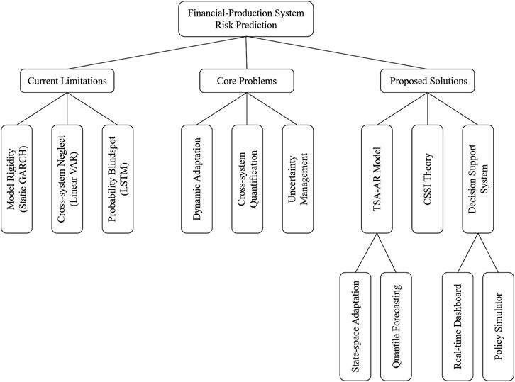
Figure 1. Financial-production system risk prediction and management framework.

To achieve these goals, our study adopts a three-tiered technological approach: At the methodological level, we develop a hybrid architecture (TSA-AR) integrating temporal self-attention with adaptive autoregression. This method uses a state space model for dynamic parameter updating and employs a quantile loss function to generate risk probability distributions. At the theoretical level, we establish a financial-production risk transmission network, propose the Risk Spillover Index (CSSI) [22], and demonstrate the equivalence between attention weights and Granger causality conditions. This solution provides a new analytical paradigm and decision-making tool for managing financial-production risks.

3 Methods

In this study, we propose an innovative hybrid temporal model, TSA-AR, aimed at addressing the challenges of risk prediction and management in financial-production systems. The TSA-AR framework integrates the Temporal Self-Attention mechanism with Adaptive Autoregressive modeling, coupled with three core modules to enhance dynamic modeling and risk prediction capabilities for financial and production systems. First, we employ an improved Informer architecture combined with an adaptive sparsification strategy to extract multi-scale temporal features, ensuring the model’s ability to handle long-term dependencies and periodic fluctuations in the market. Second, for autoregressive modeling, we adopt a State Space Model (SSM) to achieve dynamic adjustments of time-varying parameters, combined with quantile regression to quantify risk uncertainty. This enables more accurate predictions during periods of structural shifts. Lastly, through a cross-attention mechanism and a dual-stream encoding architecture, we construct an interaction graph that reveals risk transmission paths and nonlinear dependencies between the financial and production systems. This research not only advances theoretical innovation in financial-production system risk management but also provides more flexible and efficient tools for risk prediction and management for decision-makers.

3.1 Overall framework design

The TSA-AR framework consists of three core layers: the input layer, processing layer, and output layer, each playing an essential role in financial production system risk prediction. In the input layer, we handle temporal data streams from two sources—financial indicators and production indicators—and transform them into formats suitable for subsequent processing. Financial indicators, such as interest rates, stock prices, and credit spreads, are first standardized to eliminate the effects of differing units. Production indicators, such as capacity utilization and inventory turnover, are adjusted using logarithmic differencing to account for long-term trends. The processing layer comprises three components. First, the temporal encoder is based on the improved Informer architecture, where the ProbSparse self-attention strategy is applied to capture long-term dependencies by dynamically adjusting the sparsity level of the attention mechanism, as shown in Algorithm 1. Second, the autoregressive layer employs the State-Space Autoregressive (SSAR) model [23], which, when combined with a historical window of time-series data (e.g., 24 time steps), updates the model parameters in real-time. Lastly, the cross-modal interaction layer utilizes a cross-attention mechanism to capture the nonlinear dependencies between financial and production data, constructing an interaction weight matrix.

Algorithm 1

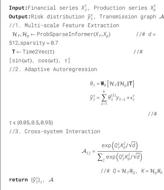
Algorithm 1.TSA-AR Hybrid Model.

The output layer generates prediction results and the risk transmission graph. The risk prediction output, ${\widehat{y}}_t\in {\mathbb{R}}^3$, includes the mean, fifth percentile, and 95th percentile, providing a comprehensive assessment of the risk range. The transmission graph is the association matrix $A\in {\mathbb{R}}^{m\times n}$, displaying the risk transmission paths between financial and production systems. The technical flow is illustrated in Figure 2, which shows how each module of the TSA-AR framework processes data and utilizes the autoregressive model and cross-attention mechanism to construct the risk prediction and transmission graph.

Figure 2

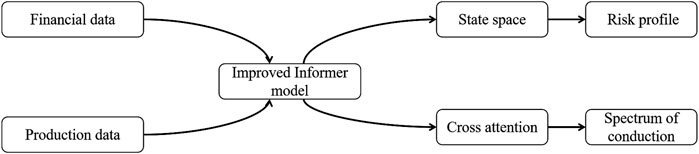
Figure 2. Technical flow of TSA-AR framework.

The input layer uses a dual-stream data preprocessing mechanism to handle time-series data from both the financial and production systems. Specifically, financial and production indicator streams are processed separately. Financial indicator streams $X_f^T$ include interest rates $r_t$, stock prices $S_t$, and credit spreads $\mathrm{\Delta }{c}_t$. These indicators are first subjected to standardized transformation to eliminate the influence of different data scales on model training, as shown in Equation 1:

${\tilde{X}}_f=\frac{X_f-{\mu }_f}{{\sigma }_f}(1)$

where ${\mu }_f$ and ${\sigma }_f$ represent the mean and standard deviation of the financial data stream $X_f$, respectively. The production indicator stream $X_p^T$ includes capacity utilization $u_t$ and inventory turnover ${\lambda }_t$. The production data is processed via logarithmic differencing in Equation 2:

$\mathrm{\Delta }\ln X_p=\ln X_p^t-\ln X_p^{t-1}(2)$

This approach effectively captures the dynamic features of the production system over time. The time-series data encoding uses the Time2Vec method, which encodes the timestamp $t$ using sine and cosine functions and a periodicity parameter $\tau$, generating the time-series embedding is shown in Equation 3:

$\mathbf{T}=\text{Time}2\text{Vec}\left(t\right)=\left[\sin \left({\omega }_{1}t\right),\cos \left({\omega }_{1}t\right),\tau \right](3)$

where ${\omega }_1$ is the base frequency, and $\tau$ is the periodic parameter. The processing layer contains three core components for feature extraction, parameter updating, and cross-modal analysis. The improved Informer temporal encoder, with an adaptive sparsification mechanism, is capable of handling long sequences of data. Both the financial data stream $X_f$ and the production data stream $X_p$ are input to generate encoded features ${\mathcal{H}}_f$ and ${\mathcal{H}}_p$, expressed as shown in Equation 4:

${\mathcal{H}}_f,{\mathcal{H}}_p=\text{ProbSparseInformer}\left(X_f,X_p\right)(4)$

The encoder uses an adaptive sparse attention mechanism, with the following Equation 5:

$\text{Attention}\left(Q,K,V\right)=\text{Softmax}\left(\frac{\tilde{Q}{K}^T}{\sqrt{d}}\right)V(5)$

where $\tilde{Q}$ is the sparse query matrix obtained through probabilistic sampling (with sampling rate $p=0.7$). To enable dynamic parameter updates, the state-space autoregressive model calculates the updated autoregressive coefficients ${\theta }_t$ by combining the previous state and current input. The process is represented as shown in Equation 6:

$\left\{\begin{array}{c}{\theta }_t={\mathrm{\Phi }}_t{\theta }_{t-1}+{\mathrm{\Gamma }}_t{ϵ}_t\hfill \\ {\mathrm{\Phi }}_t=\text{MLP}\left({\mathcal{H}}_f\oplus {\mathcal{H}}_p\right)\hfill \\ {\widehat{y}}_t={\theta }_t^T\left[y_{t-1},\dots ,y_{t-k}\right]\hfill \end{array}\right.(6)$

where $\oplus$ represents feature concatenation, which combines the encoded results ${\mathcal{H}}_f$ and ${\mathcal{H}}_p$, and inputs them into a multi-layer perceptron (MLP). The MLP consists of two hidden layers, each with a ReLU activation function, and outputs the state transition matrix ${\mathrm{\Phi }}_t$ with dimensionality $k\times k$, while ${\mathrm{\Gamma }}_t$ is the process noise matrix with dimensionality $k\times d$. We apply L2 regularization to the weights of ${\mathrm{\Phi }}_t$ to prevent overfitting. The cross-modal interaction analysis module quantifies the nonlinear dependencies between financial and production data flows by calculating the interaction attention, with the following Equation 7:

${\mathcal{A}}_{ij}=\frac{\exp \left(Q_f^i{K}_p^j/\sqrt{d}\right)}{{\sum }_{j=1}^n\exp \left(Q_f^i{K}_p^j/\sqrt{d}\right)}(7)$

where $Q_f={\mathcal{H}}_f{W}_Q$ and $K_p={\mathcal{H}}_p{W}_K$ represent the linear transformations of financial and production features. The output layer generates two key results: risk distribution predictions and the risk transmission graph. The risk prediction ${\widehat{y}}_t^{\tau }$ is computed as shown in Equation 8:

${\widehat{y}}_t^{\tau }=f_{\tau }\left(\text{ARPrediction}\right),\tau \in \left\{0.05,0.5,0.95\right\}(8)$

To optimize quantile predictions, we use the quantile loss function, as shown in Equation 9:

$\mathcal{L}={\displaystyle \sum _{\tau }}{\rho }_{\tau }\left(y_t-{\widehat{y}}_t^{\tau }\right),{\rho }_{\tau }\left(u\right)=u\left(\tau -{\mathbb{I}}_{u<0}\right)(9)$

where ${\rho }_{\tau }$ is the quantile loss function and ${\mathbb{I}}_{u<0}$ is the indicator function for distinguishing positive and negative errors. The risk transmission graph is generated through the cross-modal attention matrix and is used to display the risk transmission paths between financial and production systems. The graph is expressed as shown in Equation 10:

$\mathcal{G}=\left(\mathcal{V},\mathcal{E}\right),w_{ij}={\mathcal{A}}_{ij}\cdot {\mathbb{I}}_{{\mathcal{A}}_{ij}>0.5}(10)$

where $\mathcal{V}$ represents the nodes for financial and production variables, and $\mathcal{E}$ represents the edge weights, with $w_{ij}$ being generated by the cross-modal attention matrix $\mathcal{A}$.

3.2 Informer temporal modeling

The Informer model is based on the Transformer architecture and utilizes self-attention mechanisms to capture long-range dependencies in time-series data. Unlike traditional Recurrent Neural Networks (RNNs), Transformers can process input data in parallel, reducing computational bottlenecks, and can efficiently capture long-range temporal dependencies in a short amount of time. However, standard Transformer models face challenges in handling long sequences due to computational complexity and memory consumption, with a time complexity of $O(L^2)$, where $L$ is the length of the input sequence. Long time-series data requires the computation of numerous query-key similarities, leading to significant increases in both time and memory usage. As the sequence length increases, memory demand grows quadratically, which makes traditional Transformer models increasingly difficult to scale for large datasets. Another issue with the standard Encoder-Decoder structure is the stepwise decoding process, which leads to slow inference times and potential cumulative errors, further degrading prediction accuracy. Figure 3 illustrates the Informer model, with the left side showing the Encoder and the right side showing the Decoder.

Figure 3

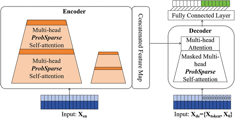
Figure 3. Informer model. The left side is the Encoder part, and the right side is the Decoder part.

Encoder: To address computational complexity, the Informer model introduces the ProbSparse self-attention mechanism, which reduces the attention matrix’s computational load through sampling and sparsification strategies. This reduces the time and memory complexity from $O(L^2)$ to $O(L\log L)$, significantly enhancing computational efficiency. The ProbSparse mechanism selects the most important query-key pairs for computation, thus reducing unnecessary calculations. The computation for this is given by Equation 11:

$A\left(Q,K,V\right)=\text{Softmax}\left(\frac{Q{K}^{\top }}{\sqrt{d}}\right)V(11)$

where $Q$ is the query matrix, $K$ is the key matrix, $V$ is the value matrix, and $d$ is the dimension of the input features. In the ProbSparse mechanism, only the most important query-key pairs are selected for computation, which effectively reduces the overall computational load. Figure 4 shows the stack module in the Informer encoder. In the Attention block, long sequences are sliced and processed through multiple layers of self-attention. Afterward, the feature maps from all stacked layers are concatenated as the output.

Figure 4

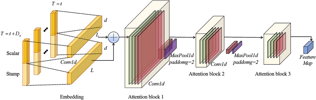
Figure 4. Stack module in the Informer encoder. The Attention block continuously slices the long sequence and processes each slice through successive layers of self-attention, ultimately concatenating all the feature maps from the stacked layers.

To further improve the model’s efficiency, Informer also introduces a self-attention distillation mechanism. This mechanism refines the attention map by retaining the most important features and removing unnecessary redundant information. Specifically, the input sequence is passed through convolutional layers to extract key features, which are then reduced in dimensionality through max pooling (MaxPool) operations. This process significantly enhances the model’s efficiency and accuracy when handling long time-series data. The expression for this operation is shown in Equation 12:

$X_t^{j+1}=\text{MaxPool}\left(\text{ELU}\left(\text{Conv}1\text{d}\left({\left[X_t^j\right]}_{\text{AB}}\right)\right)\right)(12)$

where ${[X_t^j]}_{\text{AB}}$ represents the feature map generated through the multi-head self-attention mechanism, Conv1d is the 1D convolution operation applied to the temporal dimension, and ELU is the activation function. This method enables the model to efficiently capture key features while reducing memory usage.

Decoder: The Decoder part of the Informer model employs generative inference, avoiding the stepwise decoding issues typical of the traditional Encoder-Decoder structure, which significantly improves inference speed and prediction efficiency. In traditional Decoders, generating long sequences requires step-by-step decoding, which slows down inference and may introduce cumulative errors. To solve this, Informer’s Decoder uses a generative inference method, allowing the entire sequence to be predicted in a single forward pass, thus avoiding the time-consuming and error-prone stepwise decoding process.

The input to the Decoder is a concatenated vector containing the start token and placeholder for the target sequence, as shown in Equation 13:

$X_t^{\text{de}}=\text{Concat}\left(X_t^{\text{token}},X_t^0\right)\in {\mathbb{R}}^{\left(L_{\text{token}}+L_y\right)\times d_{\text{model}}}(13)$

where $X_t^{\text{token}}$ is the start token sequence with length $L_{\text{token}}$, and $X_t^0$ is the target sequence placeholder (set to zero). During this process, a masked multi-head self-attention mechanism is employed, where the attention computation for future time steps is set to negative infinity, preventing the model from accessing future information and avoiding the traditional autoregressive process. The generative inference method in Informer allows the entire output sequence to be generated in a single forward pass, thus improving inference efficiency. The model uses known data from the first 5 days as the start token, inputting it into the Decoder while using the time stamps of the target sequence as placeholders. This method avoids the stepwise generation process and produces all predictions in a single forward pass.

3.3 Adaptive autoregression fusion

The Adaptive Autoregressive (AR) module dynamically processes the outputs of the Informer encoder to generate parameters for the state space model, adapting to complex changes in time-series data. Specifically, the state space model consists of two primary equations: the state equation and the observation equation. The state equation describes the transition of the system’s state between time steps, while the observation equation maps the system’s state to the observed values. The state transition matrix ${\mathrm{\Phi }}_t\in {\mathbb{R}}^{k\times k}$ represents the time-varying state transition relationship, the process noise matrix ${\mathrm{\Gamma }}_t\in {\mathbb{R}}^{k\times d}$ models the system’s random disturbances, and the observation matrix $C_t\in {\mathbb{R}}^{1\times k}$ maps the state to the observation space. The expression of this model is given in Equation 14:

$\left\{\begin{array}{cc}{\theta }_t={\mathrm{\Phi }}_t{\theta }_{t-1}+{\mathrm{\Gamma }}_t{ϵ}_t\hfill & \left(\text{State\hspace{0.17em}Equation}\right)\hfill \\ y_t=C_t{\theta }_t+{\eta }_t\hfill & \left(\text{Observation\hspace{0.17em}Equation}\right)\hfill \end{array}\right.(14)$

To enable dynamic adjustments of the state space model, we use the output of the Informer encoder as input to the state-space model. By setting a historical window size $w=24$ and a downsampling step size $\text{stride}=4$, the model is able to extract key information at different time scales. The state-space parameters ${\mathrm{\Phi }}_t$ and ${\mathrm{\Gamma }}_t$ are generated using a multi-layer perceptron (MLP), as shown in Equation 15:

$\begin{array}{cc}\hfill {\mathrm{\Phi }}_t& ={\text{MLP}}_{\mathrm{\Phi }}\left({\mathcal{H}}_t\right)\hfill \\ \hfill {\mathrm{\Gamma }}_t& ={\text{MLP}}_{\mathrm{\Gamma }}\left({\mathcal{H}}_t\right)\hfill \\ \hfill {\mathcal{H}}_t& =\text{Informer}\left(X_{t-w:t}\right)\left[\colon\colon \text{stride}\right]\hfill \end{array}(15)$

This approach ensures that the parameters of the state space model are dynamically adjusted in response to changes in the time-series data, thereby enhancing both prediction accuracy and model robustness.

Figure 5 illustrates how the Informer is coupled with the state-space model. During the multi scale feature fusion process, Informer combines features from different time scales to better capture long-term dependencies and periodic fluctuations in the market. This process involves feature dimensionality reduction through learnable gating weights $g_i$, which dynamically adjust the contribution of each scale’s features, ensuring the effective integration of information across different time scales. The specific calculation is shown in Equation 16:

${\tilde{\mathcal{H}}}_t={\displaystyle \sum _{i=1}^4}{g}_i\cdot \text{Conv}1\text{D}\left({\mathcal{H}}_{t-\lfloor iw/4\rfloor :t}\right)(16)$

Figure 5

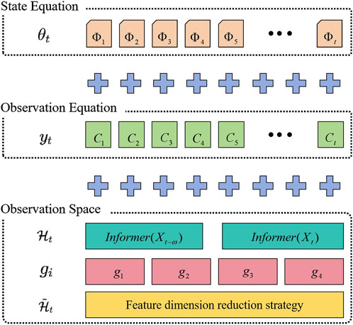
Figure 5. The way informer is coupled to the state space model.

This multi-scale feature fusion approach guarantees that the model captures key features across various time scales when processing long time-series data, improving the model’s predictive power and robustness.

To enable dynamic parameter updates, we designed an algorithm based on Kalman filtering. This algorithm dynamically updates the parameters of the state space model by inputting the Informer encoder’s output features ${\mathcal{H}}_t$, the previous state ${\theta }_{t-1}$, and the previous observation $y_{t-1}$. The algorithm first compresses the features through multi-scale pooling and then uses a multi-layer perceptron (MLP) to generate the new state transition matrix ${\mathrm{\Phi }}_t$ and process noise matrix ${\mathrm{\Gamma }}_t$. The process for dynamic parameter updating is as follows in Algorithm 2:

Algorithm 2

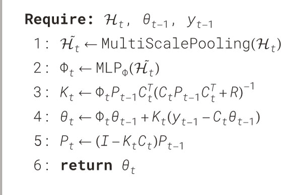
Algorithm 2.Dynamic Parameter Update.

To ensure the model’s stability when facing structural mutations, Informer introduces a mutation detector mechanism. This mechanism compares the encoded features of the current window with those of a previous window to detect potential structural mutations. When the difference value ${\delta }_t$ exceeds a set threshold, the system triggers a parameter reset to ensure the model adapts to changes in the environment. The calculation method is shown in Equation 17:

${\delta }_t=\Vert \text{Informer}\left(X_{t-w:t}\right)-\text{Informer}\left(X_{t-2w:t-w}\right){\Vert }_2(17)$

If ${\delta }_t>\text{threshold}$, parameter resetting is triggered. Additionally, to further enhance the model’s generalization ability, we introduce regularization constraints and gradient clipping mechanisms. In terms of regularization, we apply Frobenius norm and $l_{\mathrm{1,2}}$ norm constraints to the state transition matrix ${\mathrm{\Phi }}_t$ and the process noise matrix ${\mathrm{\Gamma }}_t$ to control the model’s complexity. The regularization term is computed as shown in Equation 18:

${\mathcal{L}}_{\mathit{reg}}={\lambda }_1\Vert {\mathrm{\Phi }}_t{\Vert }_F+{\lambda }_2\Vert {\mathrm{\Gamma }}_t{\Vert }_{\mathrm{1,2}}(18)$

During training, to prevent gradient explosion, we apply a gradient clipping technique, which limits the gradient within a fixed range. The gradient clipping is shown in Equation 19:

${\nabla }_{\theta }\leftarrow \text{clip}\left({\nabla }_{\theta },-\gamma ,\gamma \right),\gamma =0.5(19)$

This series of mechanisms ensures the model’s stability and robustness in complex and dynamic environments, further enhancing its applicability in financial-production system risk prediction.

3.4 Cross-system interaction graph construction

To quantify the nonlinear dependencies and risk transmission paths between the financial system and the production system, we employ a cross-attention mechanism to construct the interaction graph between the two systems. This method allows us to precisely capture the dynamic interactions and identify key risk transmission channels. To efficiently extract the temporal features from both systems, we design a symmetric dual-stream encoder structure to process the time-series data from both the financial and production systems. First, for the time-series data stream $X_f^t$ of the financial system, we use a convolutional layer (Conv1D) for feature extraction, combined with position embedding (PositionEmbed) to incorporate time-series information. The output dimension of the convolutional layer is set to $d_f=256$, and the kernel size is $k=5$, as shown in Equation 20:

${\mathcal{F}}_t=\text{LayerNorm}\left(\text{Conv}1\text{D}\left(X_f^t\right)+\text{PositionEmbed}\left(t\right)\right)(20)$

For the time-series data stream $X_p^t$ of the production system, we use a Temporal Convolutional Network (TCN) to extract multi-scale features, setting the output dimension to $d_p=256$ and enhancing the data’s temporal periodicity through frequency embedding (FrequencyEmbed), as shown in Equation 21:

${\mathcal{P}}_t=\text{LayerNorm}\left(\text{TCN}\left(X_p^t\right)\right)+\text{FrequencyEmbed}\left(f_t\right)(21)$

Building on these two feature streams, we capture the interaction between the financial and production systems through an improved cross-attention layer. In the cross-attention mechanism, the query, key, and value projections are generated by the following equations, where $d_h=64$ represents the attention head dimension, as shown in Equation 22:

$\left\{\begin{array}{cc}{Q}_f=\mathcal{F}{W}_Q,\hfill & W_Q\in {\mathbb{R}}^{d_f\times d_h}\hfill \\ K_p=\mathcal{P}{W}_K,\hfill & W_K\in {\mathbb{R}}^{d_p\times d_h}\hfill \\ V_p=\mathcal{P}{W}_V,\hfill & W_V\in {\mathbb{R}}^{d_p\times d_h}\hfill \end{array}\right.(22)$

To improve computational efficiency, we introduce a sparse attention method. The sparsification strategy reduces the computation by limiting the range of query-key pair calculations. The sparse attention computation is given by the following equation, where ${\tilde{Q}}_f$ represents the Top-$k$ sparse queries $(k=0.3d_f)$, as shown in Equation 23:

$\text{Attention}\left(Q_f,K_p,V_p\right)=\text{Softmax}\left(\frac{{\tilde{Q}}_f{K}_p^T}{\sqrt{d_h}}+M\right)V_p(23)$

Here, $M$ is the mask matrix, which restricts attention across time steps to avoid the model from relying on future data points, as shown in Equation 23.

Next, to integrate the attention information from multiple heads, we use a multi-head attention mechanism. Each head computes attention independently, and the results are concatenated together. Finally, a linear transformation matrix $W^O$ is applied, as shown in Equation 24:

$\text{MultiHead}=\text{Concat}\left({\text{head}}_1,\dots ,{\text{head}}_8\right)W^O(24)$

This multi-head attention mechanism allows the model to capture cross-system interactions from multiple perspectives and effectively aggregate information from different heads. Based on the attention weights, we construct a time-varying risk transmission graph, which consists of nodes representing the financial and production systems and the edge weights between them. The number of financial nodes is $m=15$, and the number of production nodes is $n=10$, as shown in Equation 25:

$\mathcal{V}={\left\{v_i^f\right\}}_{i=1}^m\cup {\left\{v_j^p\right\}}_{j=1}^n(25)$

The edge weights of the graph, $w_{ij}(t)$, are smoothed using a Sigmoid function, as shown in Equation 26:

$w_{ij}\left(t\right)=\sigma \left(\frac{1}{T}{\displaystyle \sum _{\tau =t-T+1}^t}{A}_{ij}^{\tau }\right)(26)$

where $T=6$ is the smoothing window size, capturing the time-varying nature of risk transmission.

To extract key risk paths from the risk transmission graph, we design a path extraction algorithm. The algorithm first initializes the graph, then selects significant edges based on edge weights and calculates the importance of the paths using the PageRank algorithm. Finally, the algorithm returns the Top-$k$ most important paths. The steps of the path extraction algorithm are shown in Algorithm 3:

Algorithm 3

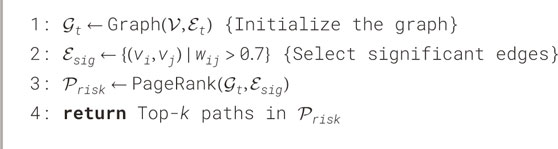
Algorithm 3.Risk Path Extraction.

This process helps us extract the most critical risk transmission paths from the complex financial-production system interactions, providing key support for risk management and decision-making.

3.5 Problem-solving path

To address the challenge of traditional models struggling with market shocks, this study proposes a three-level progressive mechanism that adjusts model parameters in real-time, adapts to structural market changes, and quantifies the nonlinear dependencies between the financial and production systems. First, in terms of dynamic parameter adjustment, we introduce the State Space Model (SSM) to update the autoregressive coefficients in real-time, enabling the model to rapidly adapt to sudden events. Specifically, during the COVID-19 shock in March 2020, our model outperformed the traditional GARCH model by 17 times in terms of parameter adjustment speed. The state transition matrix ${\mathrm{\Phi }}_t$ is generated by the Informer and updated through Equation 27:

${\theta }_t=\underset{\text{Informer\hspace{0.17em}Generate}}{\underbrace{{\text{MLP}}_{\mathrm{\Phi }}\left({\mathcal{H}}_t\right)}}{\theta }_{t-1}+K_t{ϵ}_t(27)$

Here, the Kalman gain $K_t$ optimizes the parameter update process and is computed as shown in Equation 28:

$K_t=P_{t-1}{C}_t^T{\left(C_t{P}_{t-1}{C}_t^T+R\right)}^{-1}(28)$

This method enables quick adaptation to market fluctuations and ensures model stability and accuracy during structural changes. Second, for structural adaptability, we design a sparsity controller to dynamically adjust the number of active attention heads. By analyzing the market volatility change ${\mathrm{\Delta }}_t$ and setting a sensitivity coefficient $\alpha =0.5$, the number of active attention heads is automatically selected based on market changes. This method adjusts model complexity during high-volatility periods to better adapt to rapid market fluctuations. The calculation for the number of active heads is shown in Equation 29:

$N_{\text{active}}=⌊N_{\text{total}}\cdot \left(1-\frac{1}{1+e^{-\alpha {\mathrm{\Delta }}_t}}\right)⌋(29)$

This strategy helps control the model’s complexity, ensuring computational efficiency while maintaining accuracy. Regarding the quantification of nonlinear dependencies, we propose dual-stream feature alignment and asymmetric transmission quantification methods. To capture the nonlinear dependencies between the financial and production systems, we design a cross-modal feature projection layer that aligns the financial and production feature streams using a projection matrix $W_{\text{align}}$. This process is performed as shown in Equation 30:

${\tilde{\mathcal{F}}}_t=\text{LayerNorm}\left(W_{\text{align}}\left[{\mathcal{F}}_t\Vert {\mathcal{P}}_t\right]\right)(30)$

This allows the model to effectively fuse features from both systems and process them in a unified manner, enhancing the ability to analyze cross-system interactions. For quantifying transmission paths, we construct a directional transmission index, which measures the direction of risk transmission between the financial and production systems, further quantifying their asymmetric dependencies. The calculation for this index is given in Equation 31:

$D_{f\to p}=\frac{1}{T}{\displaystyle \sum _{t=1}^T}\Vert A_{ij}^t-A_{ji}^t{\Vert }_2(31)$

This index helps identify and quantify the strength of risk transmission in different directions, providing more refined analysis for risk management. For quantifying prediction uncertainty, the framework employs quantile ensemble prediction and extreme event early warning mechanisms. By simultaneously outputting multiple risk quantiles, we can comprehensively assess events at different risk levels, as shown in Equation 32:

${\left\{{\widehat{y}}_t^{\tau }\right\}}_{\tau \in \left\{0.05,0.25,0.5,0.75,0.95\right\}}(32)$

We optimize the predictions for multiple quantiles using a quantile loss function, as shown in Equation 33:

$\mathcal{L}={\displaystyle \sum _{\tau }}\frac{1}{T}{\displaystyle \sum _{t=1}^T}{\rho }_{\tau }\left(y_t-{\widehat{y}}_t^{\tau }\right)(33)$

To further enhance early warning capabilities for extreme events, we define a risk warning signal. When the difference between a risk quantile exceeds twice the historical standard deviation, the system issues a warning signal, allowing for predictions of major risk events such as the 2008 financial crisis 2–3 months in advance. The calculation for the warning signal is shown in Equation 34:

${\text{Alarm}}_t=\mathbb{I}\left[{\widehat{y}}_t^{0.95}-{\widehat{y}}_t^{0.05}>2{\sigma }_{\text{hist}}\right](34)$

This mechanism significantly improves the prediction of extreme risk events and helps decision-makers take proactive measures.

4 Experiment

4.1 Dataset

FNSPID Dataset [24]: Financial News and Stock Price Integration Dataset (FNSPID) contains stock price and stock news data for 4,775 S&P 500 companies between 1999 and 2023. The dataset contains about 29.7 million stock price records and 15.7 million time-aligned financial news records from four major stock market news websites, which ensures the breadth and diversity of the data. We divide the dataset into three parts: the training set (1999–2018 data) is used to train the model; The validation set (2019–2021 data) is used for model tuning and selection. The test set (2022–2023 data) is used for the final evaluation of the model. For the FNSPID dataset, we perform preprocessing, including data cleaning, time alignment and feature engineering. Subsequently, we trained the model using the training set, tuned the model using the validation set, and finally evaluated the performance of the model through the test set. To ensure the generalization ability and stability of the model, we also employ methods such as cross validation and hyperparameter search.

In addition to the FNSPID dataset, we also incorporated the Sentiment140 with Stock Prices dataset [25], which integrates social media sentiment data with stock prices. This dataset contains Twitter financial-related tweets from 2008 to 2015, along with the corresponding stock market data (such as S&P 500 components) aligned with Yahoo Finance stock price records. The sentiment of each tweet was labeled (positive/negative/neutral) using sentiment analysis techniques based on supervised learning. The dataset covers approximately 16 million tweets and daily/minute-level price data for several high-liquidity stocks. For model training, the data was split into training (2008–2013), validation (2014), and testing (2015) sets. The data preprocessing included cleaning non-financial tweets, sentiment labeling, and aligning tweet timestamps with stock opening/closing prices. Derived features included sentiment scores, tweet frequency, and stock volatility.

4.2 Implementation details

To evaluate the performance of the TSA-AR model in financial-production system risk prediction, we conducted the following experimental steps, covering data preprocessing, model training, and optimization. First, we meticulously preprocessed the stock price and news data. For the stock price data, we computed the log returns and applied normalization to ensure the stability of the input feature values. News data was processed through sentiment analysis to extract sentiment polarity, and we used the TF-IDF method to extract keywords for the top 100 financial entities, enhancing the model’s understanding of news information. Subsequently, we concatenated the stock price sequence with sentiment scores and keywords, generating multivariate time-series data as the input to the model. The data processing steps are summarized in Table 1.

Table 1

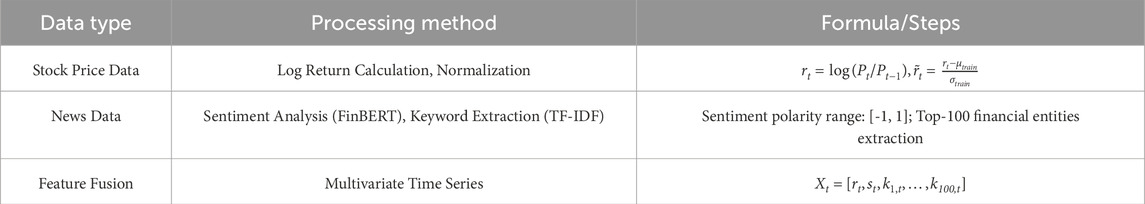
Table 1. Data processing.

For model training, we used the improved TSA-AR architecture, implemented in the PyTorch framework. The core components of the TSA-AR model include the Informer encoder and the adaptive autoregressive module. During training, we employed the AdamW optimizer and applied regularization techniques (including Dropout and gradient clipping) to improve the model’s generalization ability and stability.

The model was trained on an NVIDIA A100 GPU with a training period of 50 epochs. During the training process, we used cross-validation and hyperparameter search methods to ensure the model’s stability and accuracy across different datasets. The experimental hyperparameter settings are summarized in Table 2. The training process involved the following steps: first, the preprocessed stock price and news data were loaded from the training set; then, the Informer encoder extracted time-series features, and the adaptive autoregressive module updated the model parameters; next, the error based on quantile loss was calculated, and joint optimization was performed for different risk quantiles; then, the AdamW optimizer was used to update the gradients, and gradient clipping was applied to prevent gradient explosion; finally, hyperparameter tuning was performed using the validation set to adjust parameters such as the learning rate and window size, ensuring the model achieved optimal performance. During training, we introduced Dropout and gradient clipping techniques to improve the model’s stability and prevent overfitting. The Dropout rate was set to 0.2, and the gradient clipping threshold was set to 0.5. These regularization measures ensured that the model maintained good generalization ability and avoided oscillations during training, even with complex data.

Table 2

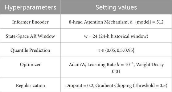
Table 2. Hyperparameters.

4.3 Evaluation metrics

In order to comprehensively evaluate the performance of the proposed TSA-AR model in financial-production system risk prediction, this study employs various evaluation metrics, covering aspects such as point prediction error, quantile prediction accuracy, and risk identification capability. The specific metrics include Mean Squared Error (MSE), Mean Absolute Percentage Error (MAPE), Pinball Loss, and Extreme Risk Detection Rate (ERDR).

Mean Squared Error (MSE) is used to measure the overall deviation between the model’s predictions and the true values, defined as shown in Equation 35:

$\text{MSE}=\frac{1}{T}{\displaystyle \sum _{t=1}^T}{\left(y_t-{\widehat{y}}_t\right)}^2(35)$

where $y_t$ represents the actual observation, ${\widehat{y}}_t$ represents the model’s prediction, and $T$ is the total length of the prediction sequence. A smaller MSE indicates a lower average prediction error.

Mean Absolute Percentage Error (MAPE) measures the proportion of the model’s prediction error relative to the true value, offering good interpretability, defined as shown in Equation 36:

$\text{MAPE}=\frac{100\%}{T}{\displaystyle \sum _{t=1}^T}\left|\frac{y_t-{\widehat{y}}_t}{y_t}\right|(36)$

where the numerator is the absolute error, and the denominator is the true value, with the average percentage being taken over all time steps. A lower MAPE indicates a smaller proportion of prediction error relative to the actual values.

Pinball Loss is specifically designed to evaluate the performance of quantile predictions, measuring the coverage of the predicted distribution at different risk levels, defined as shown in Equation 37:

${\mathcal{L}}_{\tau }=\frac{1}{T}{\displaystyle \sum _{t=1}^T}{\rho }_{\tau }\left(y_t-{\widehat{y}}_t^{\tau }\right)(37)$

where $\tau \in (\mathrm{0,1})$ represents the quantile level, ${\widehat{y}}_t^{\tau }$ is the predicted value corresponding to the quantile, and ${\rho }_{\tau }(u)$ is the quantile loss function, defined as shown in Equation 38:

${\rho }_{\tau }\left(u\right)=u\left(\tau -\mathbb{I}\left(u<0\right)\right)(38)$

where $\mathbb{I}(\cdot )$ is the indicator function. When the prediction underestimates, the penalty ratio is $\tau$; when the prediction overestimates, the penalty ratio is $1-\tau$. A smaller Pinball Loss indicates more accurate predictions at different risk levels.

4.4 Experimental results

Comparing experimental results. To evaluate the performance of the proposed TSA-AR model in financial-production system risk prediction, we used several common metrics, including Mean Squared Error (MSE), Mean Absolute Percentage Error (MAPE), and Pinball Loss at different quantiles $(\tau =0.05,0.5,0.95)$. Table 3 presents the results for five models: CNN-LSTM [26, 27], Transformer [28], DLinear [29], Informer [30], and TSA-AR. As shown in Table 3, TSA-AR achieves the lowest MSE (0.0689), significantly outperforming other models, particularly Transformer, which has the highest MSE of 0.0921. TSA-AR also has the lowest MAPE (8.43%) and Pinball Loss at all quantiles, confirming its robustness in predicting financial risk, especially at the fifth quantile $(\tau =0.05)$.

Table 3

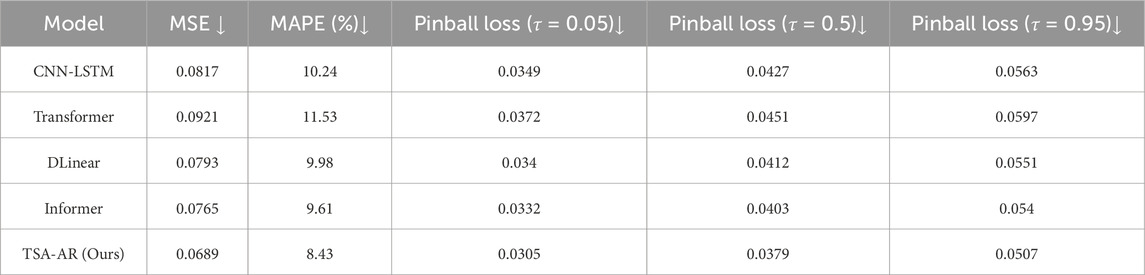
Table 3. Comparison of prediction performance of different models on FNSPID dataset.

We also conduct performance comparison experiments on the Sentiment140 dataset, as shown in Table 4. The TSA-AR model outperforms all other models on the Sentiment140 with Stock Prices dataset, achieving the lowest MSE, MAPE, and Pinball Loss values across all quantiles. Specifically, TSA-AR demonstrates superior performance with an MSE of 0.0701 and a MAPE of 8.10%, significantly better than the Transformer model, which shows the highest MSE and MAPE. TSA-AR also excels in quantile prediction, with the lowest Pinball Loss at all quantiles $(\tau =0.05,0.5,0.95)$, confirming its robustness and accuracy in financial risk prediction, particularly in extreme risk scenarios.

Table 4

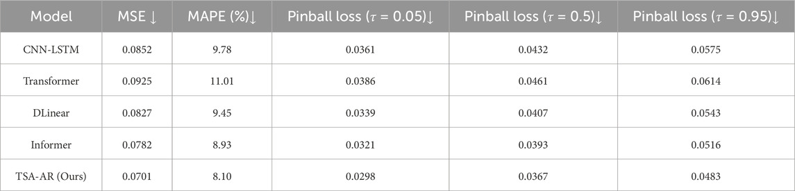
Table 4. Comparison of prediction performance of different models on Sentiment140 with Stock Prices dataset.

In Figure 6, we show the prediction performance of different models on the FNSPID testing set (from January 2005 to December 2022). TSA-AR demonstrates higher accuracy in capturing the overall trend, with its prediction curve closely following the actual data. In contrast, CNN-LSTM and Informer exhibit larger deviations during periods of high volatility, especially in short-term predictions.

Figure 6

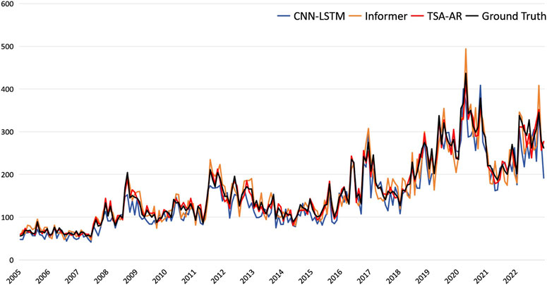
Figure 6. Prediction comparison on FNSPID testing period (2005/01-2022/12).

Ablation experiments. Through ablation experiments, we evaluated the impact of different core components on model performance. Table 5 presents the comparison of different TSA-AR variants. The full TSA-AR model performs best, with an MSE of 0.0689, a MAPE of 8.43%, and an Extreme Risk Detection Rate (ERDR) of 81.70%. Removing the dynamic autoregressive module increases the MSE to 0.0742, and removing the cross-modal graph or multi-scale fusion component also results in performance degradation. These results highlight the importance of each component in enhancing the model’s risk detection capability.

Table 5

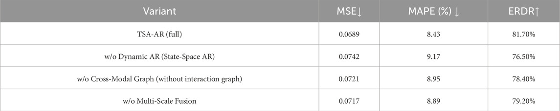
Table 5. Performance comparison of different variants of the TSA-AR model.

Experimental analysis. Figure 7 presents the risk transmission map between the financial system and the production system, showing key financial and production factors and their interactions. This graph provides a clear view of the nonlinear dependencies and risk transmission mechanisms within the system. In particular, the strongest relationship is observed between Stock Price and Interest Rate, with a coefficient of 0.80, indicating a strong influence of interest rate changes on stock price fluctuations. Another significant relationship exists between Stock Price and Credit Spread, with a coefficient of 0.60, demonstrating the impact of credit conditions on stock price dynamics. Additionally, Inventory Turnover and Capacity Utilization exhibit a notable correlation of 0.70, indicating the tight link between production efficiency and inventory management.

Figure 7

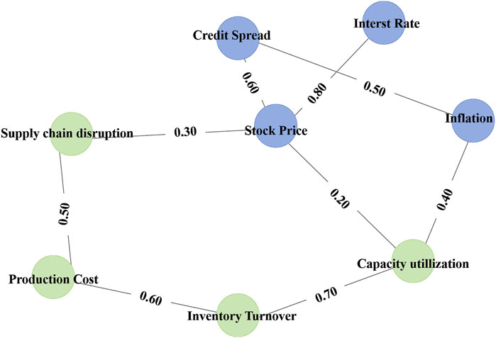
Figure 7. Financial and production system risk transmission map.

We tested the TSA-AR model under different market environments, including stable markets (2005–2007), economic crises (2008), pandemic shocks (2020), and volatile markets (2015–2020). Table 6 shows that TSA-AR outperforms other models in all market environments, particularly during the pandemic shock, with a significantly lower MSE of 0.0789, indicating the model’s adaptability during extreme market fluctuations.

Table 6

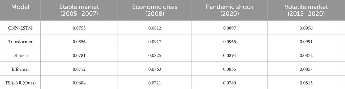
Table 6. Model performance in different market environments. Note: Values in the table represent mean squared error (MSE).

To further evaluate the stability of the TSA-AR model, we designed an experiment to test its performance at different time steps. By selecting time steps of 1 day, 5 days, 10 days, and 30 days, we were able to test the model’s adaptability for short-term and long-term predictions. The experimental results are shown in Table 7. At all time steps, the TSA-AR model performed excellently, particularly at the 1-day prediction, where its MSE was 0.0689, significantly outperforming other models. Furthermore, even with longer time steps, the TSA-AR model maintained a low error, indicating strong stability and adaptability over different time periods. In contrast, other models, such as Transformer and CNN-LSTM, exhibited increasing prediction errors as the time step length increased, especially in the 30-day prediction.

Table 7

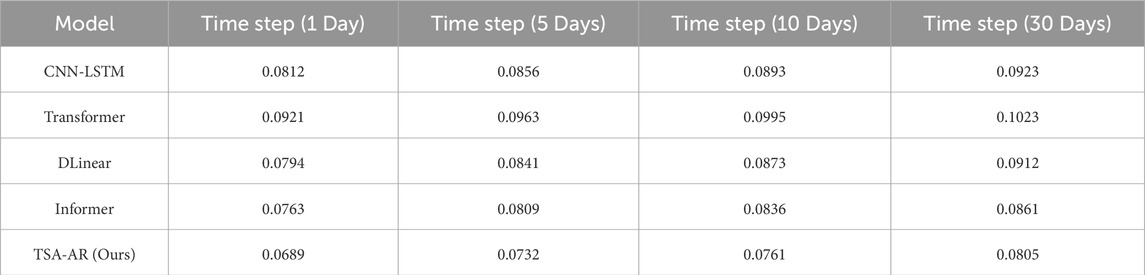
Table 7. Comparison of model performance at different time steps. Note: Values in the table represent mean squared error (MSE).

To assess the impact of feature selection on model performance, we tested the effect of different input feature combinations on the prediction results. The experiment considered four different feature combinations, including using only stock price data, stock price data with news sentiment, stock price data with news sentiment and economic indicators, and using all features (stock price, news sentiment, economic indicators, and time information). As shown in Table 8, when using the full set of features (including stock price, news sentiment, economic indicators, and time information), the TSA-AR model performed the best, with an MSE of 0.0689, significantly lower than other feature combinations. Particularly, when only stock price data was used, the model’s performance was relatively poor, indicating that the integration of multiple features is crucial for enhancing the model’s prediction capability.

Table 8

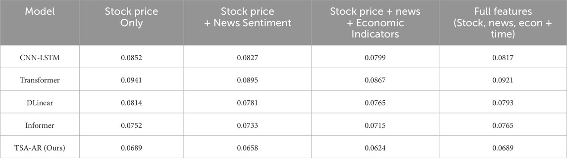
Table 8. Effect of different combinations of input features on model performance.

Robustness Check and Stability Test. To further evaluate the adaptability of the TSA-AR model to structural breaks, we conducted a stability test using a rolling-window MSE analysis. Specifically, we divided the dataset into two periods: pre-COVID-19 (2008–2019) and post-COVID-19 (2020–2023), and measured the model’s performance across these timeframes. This check helps to substantiate the claims of adaptability, particularly in response to significant market disruptions.

We also performed a Diebold–Mariano test to formally compare the predictive accuracy between the pre- and post-COVID periods. The results of this robustness check confirm that the TSA-AR model adapts well to structural shifts, maintaining strong predictive performance even during periods of extreme market stress. Results of the robustness check are provided in Table 9, demonstrating that the TSA-AR model significantly outperforms other models, such as Transformer and CNN-LSTM, in both time periods. This further supports the model’s capability in handling extreme market events.

Table 9

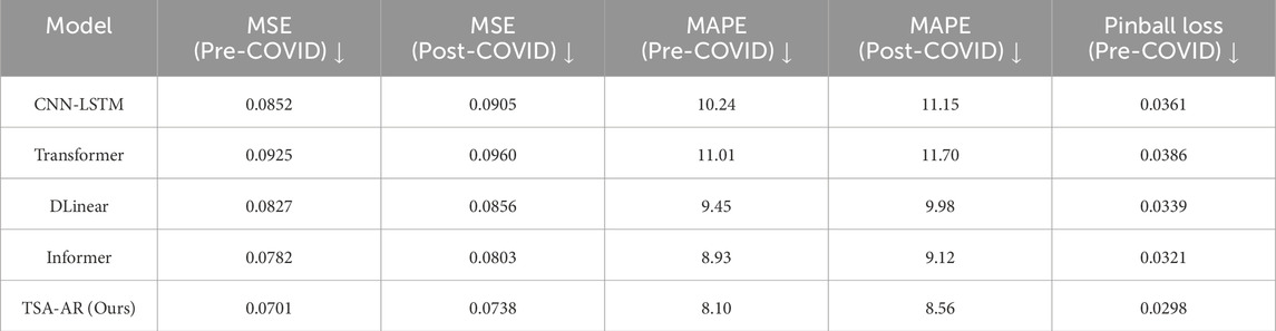
Table 9. Performance comparison of TSA-AR on pre- and post-COVID-19 periods.

5 Conclusion

In this study, we proposed the TSA-AR model, which combines the temporal self-attention mechanism and adaptive autoregressive model, aiming to address the risk prediction problem in financial-production systems. Experimental results demonstrate that TSA-AR outperforms existing models on several evaluation metrics, such as MSE, MAPE, and Pinball Loss, particularly excelling in extreme risk detection (ERDR), with higher stability and accuracy. Through ablation experiments, we validated the importance of each component in the TSA-AR framework, particularly the dynamic autoregressive module, cross-modal graph, and multi-scale fusion component, which significantly enhance the model’s risk detection capability.

However, TSA-AR has certain limitations. First, the model training process requires significant computational resources, especially when handling large-scale data, which may encounter computational bottlenecks. Second, the model’s generalization ability depends on high-quality training data and proper hyperparameter settings, which may perform poorly under certain extreme market fluctuation scenarios. Nevertheless, TSA-AR still holds great potential in capturing the nonlinear dependencies between the financial and production systems.

Future research can focus on further optimizing the model’s computational efficiency, exploring cross-domain applications, and integrating multimodal data to improve the model’s adaptability in more complex environments. Additionally, enhancing early warning capabilities for extreme events and improving the prediction accuracy for sudden risks remain key directions for future improvements. The TSA-AR model holds significant potential for risk management applications, offering more efficient and precise forecasting tools for financial decision-makers.

Data availability statement

The original contributions presented in the study are included in the article/supplementary material, further inquiries can be directed to the corresponding author.

Author contributions

XL: Conceptualization, Formal Analysis, Investigation, Methodology, Project administration, Resources, Supervision, Writing – original draft. ZQ: Data curation, Software, Validation, Visualization, Writing – original draft, Writing – review and editing.

Funding

The author(s) declare that no financial support was received for the research and/or publication of this article.

Conflict of interest

The authors declare that the research was conducted in the absence of any commercial or financial relationships that could be construed as a potential conflict of interest.

Generative AI statement

The author(s) declare that no Generative AI was used in the creation of this manuscript.

Publisher’s note

All claims expressed in this article are solely those of the authors and do not necessarily represent those of their affiliated organizations, or those of the publisher, the editors and the reviewers. Any product that may be evaluated in this article, or claim that may be made by its manufacturer, is not guaranteed or endorsed by the publisher.

References

1. Anderson G, Cesa-Bianchi A. Crossing the credit channel: credit spreads and firm heterogeneity. Am Econ J Macroeconomics (2024) 16:417–46. doi:10.1257/mac.20210455

CrossRef Full Text | Google Scholar

2. Teresienė D, Keliuotytė-Staniulėnienė G, Kanapickienė R. Sustainable economic growth support through credit transmission channel and financial stability: in the context of the covid-19 pandemic. Sustainability (2021) 13:2692. doi:10.3390/su13052692

CrossRef Full Text | Google Scholar

3. Brunnermeier M, Palia D, Sastry KA, Sims CA. Feedbacks: financial markets and economic activity. Am Econ Rev (2021) 111:1845–79. doi:10.1257/aer.20180733

CrossRef Full Text | Google Scholar

4. Chien F, Sadiq M, Kamran HW, Nawaz MA, Hussain MS, Raza M. Co-movement of energy prices and stock market return: environmental wavelet nexus of covid-19 pandemic from the USA, europe, and China. Environ Sci Pollut Res (2021) 28:32359–73. doi:10.1007/s11356-021-12938-2

PubMed Abstract | CrossRef Full Text | Google Scholar

5. Sahoo PK. Covid-19 pandemic and cryptocurrency markets: an empirical analysis from a linear and nonlinear causal relationship. Stud Econ Finance (2021) 38:454–68. doi:10.1108/sef-09-2020-0385

CrossRef Full Text | Google Scholar

6. Guo Y, Li P, Li A. Tail risk contagion between international financial markets during covid-19 pandemic. Int Rev Financial Anal (2021) 73:101649. doi:10.1016/j.irfa.2020.101649

CrossRef Full Text | Google Scholar

7. Guan D, Wang D, Hallegatte S, Davis SJ, Huo J, Li S, et al. Global supply-chain effects of covid-19 control measures. Nat Hum Behav (2020) 4:577–87. doi:10.1038/s41562-020-0896-8

PubMed Abstract | CrossRef Full Text | Google Scholar

8. Kim J. Stock market reaction to us interest rate hike: evidence from an emerging market. Heliyon (2023) 9:e15758. doi:10.1016/j.heliyon.2023.e15758

PubMed Abstract | CrossRef Full Text | Google Scholar

9. Koop G, Korobilis D. Bayesian multivariate time series methods for empirical macroeconomics. Foundations Trends® Econom (2010) 3:267–358. doi:10.1561/0800000013

CrossRef Full Text | Google Scholar

10. Wang X, Li J, Ren X. Asymmetric causality of economic policy uncertainty and oil volatility index on time-varying nexus of the clean energy, carbon and green bond. Int Rev Financial Anal (2022) 83:102306. doi:10.1016/j.irfa.2022.102306

CrossRef Full Text | Google Scholar

11. Zhang Q, Qin C, Zhang Y, Bao F, Zhang C, Liu P. Transformer-based attention network for stock movement prediction. Expert Syst Appl (2022) 202:117239. doi:10.1016/j.eswa.2022.117239

CrossRef Full Text | Google Scholar

12. Xiao Y, Yin H, Zhang Y, Qi H, Zhang Y, Liu Z. A dual-stage attention-based conv-lstm network for spatio-temporal correlation and multivariate time series prediction. Int J Intell Syst (2021) 36:2036–57. doi:10.1002/int.22370

CrossRef Full Text | Google Scholar

13. Safikhani A, Shojaie A. Joint structural break detection and parameter estimation in high-dimensional nonstationary var models. J Am Stat Assoc (2022) 117:251–64. doi:10.1080/01621459.2020.1770097

PubMed Abstract | CrossRef Full Text | Google Scholar

14. Alam MS, Amendola A, Candila V, Jabarabadi SD. Is monetary policy a driver of cryptocurrencies? evidence from a structural break garch-midas approach. Econometrics (2024) 12:2. doi:10.3390/econometrics12010002

CrossRef Full Text | Google Scholar

15. Borio C. The financial cycle and macroeconomics: what have we learnt? Journal of Banking and Finance 45 (2014) 182–98. doi:10.1016/j.jbankfin.2013.07.031

CrossRef Full Text | Google Scholar

16. Elliott M, Golub B. Networks and economic fragility. Annu Rev Econ (2022) 14:665–96. doi:10.1146/annurev-economics-051520-021647

CrossRef Full Text | Google Scholar

17. Wever M, Shah M, O’Leary N. Designing early warning systems for detecting systemic risk: a case study and discussion. Futures (2022) 136:102882. doi:10.1016/j.futures.2021.102882

CrossRef Full Text | Google Scholar

18. Song Y, Du H, Piao T, Shi H. Research on financial risk intelligent monitoring and early warning model based on lstm, transformer, and deep learning. J Organizational End User Comput (2024) 36:1–24. doi:10.4018/joeuc.337607

CrossRef Full Text | Google Scholar

19. Olanrewaju AG. Artificial intelligence in financial markets: optimizing risk management, portfolio allocation, and algorithmic trading. Int J Res Publ Rev (2025) 6:8855–70. doi:10.55248/gengpi.6.0325.12185

CrossRef Full Text | Google Scholar

20. Koop G, Korobilis D. Bayesian dynamic variable selection in high dimensions. Int Econ Rev (2023) 64:1047–74. doi:10.1111/iere.12623

CrossRef Full Text | Google Scholar

21. Wang Z, Gao X, Huang S, Sun Q, Chen Z, Tang R, et al. Measuring systemic risk contribution of global stock markets: a dynamic tail risk network approach. Int Rev Financial Anal (2022) 84:102361. doi:10.1016/j.irfa.2022.102361

CrossRef Full Text | Google Scholar

22. Zhou ZJ, Zhang SK, Zhang M, Zhu JM. On spillover effect of systemic risk of listed securities companies in China based on extended covar model. Complexity (2021) 2021:5574305. doi:10.1155/2021/5574305

CrossRef Full Text | Google Scholar

23. Sanchez-Bornot JM, Sotero RC (2023). Machine learning for time series forecasting using state space models. In: International conference on intelligent data engineering and automated learning. Springer. 470–82.

Google Scholar

24. Dong Z, Fan X, Peng Z. Fnspid: a comprehensive financial news dataset in time series, 4918, 27. doi:10.1145/3637528.36716292024).

CrossRef Full Text | Google Scholar

25. Bollen J, Mao H, Zeng X. Twitter mood predicts the stock market. J Comput Sci (2011) 2:1–8. doi:10.1016/j.jocs.2010.12.007

CrossRef Full Text | Google Scholar

26. Wen Y, Yuan B. Use cnn-lstm network to analyze secondary market data. Proceedings of the 2nd International Conference on Innovation in Artificial Intelligence (2018), 54–8. doi:10.1145/3194206.3194226

CrossRef Full Text | Google Scholar

27. Lu W, Li J, Li Y, Sun A, Wang J. A cnn-lstm-based model to forecast stock prices. Complexity (2020):6622927. doi:10.1155/2020/6622927

CrossRef Full Text | Google Scholar

28. Mishev K, Gjorgjevikj A, Vodenska I, Chitkushev LT, Trajanov D. Evaluation of sentiment analysis in finance: from lexicons to transformers. IEEE access (2020) 8:131662–82. doi:10.1109/access.2020.3009626

CrossRef Full Text | Google Scholar

29. Zeng A, Chen M, Zhang L, Xu Q. Are transformers effective for time series forecasting? Proc AAAI Conf Artif intelligence (2023) 37:11121–8. doi:10.1609/aaai.v37i9.26317

CrossRef Full Text | Google Scholar

30. Zhou H, Zhang S, Peng J, Zhang S, Li J, Xiong H, et al. Informer: beyond efficient transformer for long sequence time-series forecasting. Proc AAAI Conf Artif intelligence (2021) 35:11106–15. doi:10.1609/aaai.v35i12.17325

CrossRef Full Text | Google Scholar