Operationalizing fractal linguistics: toward a unified framework for cross-disciplinary fractal analysis

1 Introduction

Fractal analysis has become an essential tool in multiple scientific disciplines, including physics, biology, neuroscience, medicine, biomedical engineering, materials science, economics, and environmental sciences, to name a few. The concept was first proposed by Mandelbrot (1983), based on the self-similarity of structures across different scales that are not definable by Euclidean geometry [1–3].

However, despite its widespread application, the precise definition and interpretation of fractal-related concepts remain inconsistent across disciplines [2,4–7]. Terms such as “fractal dimension,” “self-similarity,” “self-affinity,” “roughness,” “scaling laws,” the role of embedding dimension and topological dimension in spatial contexts are frequently applied in contexts where their mathematical rigor is uncertain [8–10]. This has led to a semantic drift in scientific discourse, creating barriers to effective interdisciplinary communication [11,12]. Addressing this, a differentiation between fractal analysis and fractal synthesis has been suggested, where fractal analysis focuses on single-dimension metrics to measure the complexity of an image or time series, whereas fractal synthesis combines local and global dimensions, entropy, and spatial-temporal dynamics to establish a more comprehensive understanding of complex systems. To take this further, this manuscript addresses the technical foundations and methodologies required to reliably interpret fractal descriptions by addressing assumptions of stationarity, selection of scale range, and use of surrogate data testing.

2 Complexity of image and time series data

2.1 Scale and measurement in fractal analysis

Before the advent of fractal analysis, Richardson (1961) explored the relationship between scale and length in coastlines, demonstrating that coastline length increases as measurement scale decreases, following a power-law relationship [13]. The exponent in this relationship quantifies the rate at which length changes with scale, forming the foundation of fractal dimension analysis [3,14]. This early work laid the foundation for modern fractal analysis, which employs techniques such as box-counting, dilation, mass-radius, and the caliper method [5,15–17]. These methods all serve as analytical tools that estimate object size or mass with the measurement scale and collectively form the basis of fractal analysis. The key exponent in these relationships, termed the fractal dimension (D_E), characterizes the complexity of an object’s scaling properties. However, there is ongoing debate regarding what constitutes a “dimension” in mathematical and physical sciences. While the Hausdorff dimension is mathematically rigorous, other fractal dimensions, such as Minkowski and Kolmogorov dimensions, are widely used in applied fields despite not meeting strict mathematical definitions [18,19].

Many traditional fractal analysis methods, such as box-counting, assume a well-defined structure within an image or dataset, which does not always translate well to nonlinear and self-affine time-series data. Multifractal detrended fluctuation analysis (MF-DFA) has been introduced to account for these variations but remains sensitive to preprocessing techniques and data resolution, leading to the proposal of diverse multiscaling or multifractal applications [20–30].

A fundamental aspect of fractal analysis when applying DFA or box-counting is the selection of an appropriate scaling range. A shortcoming of DFA is that it assumes stationarity within each detrending window (see below for mathematical treatment). However, this is not always found in physiological time series, which leads to incorrect inferences of fractality. Testing goodness-of-fit and ensuring the correct polynomial detrending order to avoid under- or overfitting provides robust results [31].

2.2 Applications of fractal analysis across scientific fields

Fractal analysis has been employed across a wide spectrum of scientific and technological endeavors as well as in the arts. One of the possibly best-known applications of fractal analysis in the arts was the identification of a fractal-like pattern in the artistic work of Jackson Pollock and the Mandelbrot set [4,32–34]. Differences in different schools of Orthodox iconography and fractal analysis of scribal and ink identification also have a connection to fractal analysis [35,36]. Connected to the arts is the built-up environment [2,37]. From the very large scales to the molecular scale, solar and space physics use fractal approaches to model solar flare distributions, solar wind turbulence, and magnetospheric dynamics. In thermodynamics, fractal analysis deals with the molecular or atomic level [38–40]. From thermodynamics, combustion theory can be understood, where fractals describe flame front irregularities and turbulent eddies [41–44]. In materials science, fractal models describe grain boundary growth and porous structure distributions [45]. Liquid crystal textures exhibit fractal patterns during phase transitions [46]. Statistical physics incorporates fractals to describe anomalous diffusion and scaling in critical phenomena [47]. In geophysics and environmental sciences, fractals appear in models of porous media, glaciology (crevasse networks and ice-sheet roughness), and sedimentary layering [48,49]. Earthquake prediction research uses fractal statistics to characterize fault systems and seismicity patterns [50]. Ocean dynamics, river basin distribution patterns, and tsunami wave modeling leverage fractal structures to capture nonlinear wave propagation and coastline complexity [51,52]. Climate science is another related area of research utilizing fractal analysis principles [53–55]. In finance, fractal analysis is applied to market time series to understand volatility clustering and multifractal structures in asset returns. This rather limited overview of the wide-ranging applications highlights the need for a standardized methodological framework across disciplines. From the previous paragraphs and the citations, it becomes apparent that, for instance, the term “roughness” is quite common to describe surface complexity, yet roughness as discussed later is not a fractal property. The current paper concentrates on physiological processes and morphology related to fractal analysis and argues for a consistent use of definitions.

2.3 Fractal analysis of temporal signals

Beyond spatial applications, fractal analysis has been increasingly applied to physiological time-series data that can be analyzed by several different methods, briefly highlighted in this section [35,56]. Similar to geometric fractals, time-series fractals exhibit scale invariance in their temporal fluctuations, which can be analyzed using a variety of techniques such as detrended fluctuation analysis (DFA), Hurst exponent estimation, wavelet transforms, Higuchi algorithm, diverse entropy-based methods, and symbolic dynamics [30,57–73]. These methods have been linked to understanding neurological function, cardiovascular health, and autonomic regulation which address diverse pathologies including stroke, cardiovascular disease (CVD), mental health disorders, and diabetes, amongst many others.

The Hurst exponent (H) is a classical measure of the persistence or anti-persistence of a time series, including rescaled range (R/S) analysis [74]. It quantifies whether a system exhibits memory effects, where H < 0.5 indicates anti-persistent behavior, H = 0.5 suggests randomness, and H > 0.5 denotes long-range dependence. An often-not-considered aspect of the Hurst exponent is that the traditional Hurst exponent estimation assumes stationarity. This has been addressed by the Hurst-Kolmogorov (HK) method used for estimating the Hurst exponent. The HK method accurately assesses long-range correlations when the measurement time series is short, shows minimal dispersion about the central tendency, and yields a point estimate that does not depend on the length of the measurement time series or its underlying Hurst exponent [75]. Another difficulty in determining the Hurst coefficient is that the computation of H depends on the signal type [31,76]. The signal type can be fractional Gaussian noise ($fGn$) or fractional Brownian motion ($fBm$), where mathematically $fGn$ is the first derivative of $fBm$, and $fBm$ is the temporal integral of $fGn$. $fGn$ is stationary with zero mean and short or long-range correlations, depending on the Hurst exponent $fGn$ has slopes of the power spectral density (PSD) smaller than one ($\beta <1$), where $\beta$ is the spectral exponent (slope of power spectral density). Whereas $fBm$ is non-stationary and is self-similar with long-range dependence and increasing variance over time with slope greater than one ($\beta$ >1) [77]. The power spectral density (PSD) is then defined as:

$S\left(f\right)\propto f^{-\beta }$

where $f$ is frequency and $b$ is the scaling exponent, which indicates the complexity of the signal [31,78].

The spectral power exponent is defined through the PSD and indicates how energy or power is distributed across frequencies in a signal and characterizes the scale-invariance and fractal properties in temporal dynamics. $\beta$ indicates signal complexity and is linked to the long-term correlations of the signal. As such $\beta$ defines white noise, which is a completely uncorrelated time series $\beta =0$. Pink or $1/f$ noise has correlated fluctuations and is defined as $0<\beta <1$. $\beta$ being greater than 0.5 indicates persistent Brownian motion, whilst $\beta$ less than 0.5 indicates anti-persistent Brownian motion. When $\beta =2$, the signal is akin to Brownian motion and exhibits non-stationary time evolution. Brownian motion and stronger persistence, with less local variability, are associated with $\beta >2$ [77]. From a fractal perspective, $\beta$ reflects the self-affinity of the signal and signals with higher $\beta$ exhibit smoother, more correlated behavior, whereas lower $\beta$ implies higher-frequency fluctuations and greater complexity.

$\left(fBm\right.$) generalizes classical Brownian motion by introducing memory via the Hurst exponent H∈(0,1), which controls the degree of long-range dependence and smoothness. Mandelbrot and van Ness originally defined this process as:

$B_H\left(t\right)=\frac{1}{\mathrm{\Gamma }\left(H+\frac{1}{2}\right)}\left[{\int }_{-\infty }^0\left\{{\left(t-s\right)}^{H-\frac{1}{2}}-{\left(-s\right)}^{H-\frac{1}{2}}\right\}dW\left(s\right)+{\int }_0^t{\left(t-s\right)}^{H-\frac{1}{2}}dW\left(s\right)\right]$

The $B_H\left(t\right)$ process is self-similar with stationary moments, where $B_H\left(t\right)$ is the fractional Brownian motion with Hurst exponent $H$; $\mathrm{\Gamma }\left(·\right)$ is the Gamma function, $W\left(s\right)$ is the standard Wiener process (Brownian motion) and $H\in \left(0,1\right)$ determines the correlation structure. $H=5$ is standard Brownian motion with no memory. $H>5\&H<5$ indicates persistent behavior and anti-persistent behavior, respectively [31,79]. $B_H\left(t\right)$ is a specific process, which is referred to as normal $fBm$ ($nfBm$) in the mathematical literature and emphasizes that it is a Gaussian process in the statistical sense. $nfBm$ adheres strictly to the Mandelbrot and van Ness (MvN) definition and distinguishes this definition from other generalizations or $fBm$-like processes. The current paper uses $fBm$ consistently in the MvN sense.

The Hurst coefficient for $fGn$ is calculated with $H=\frac{\beta +1}{2}$ for $fGn$ and with $H=\frac{\beta -1}{2}$ for $fBm$ signals, see [31]. This results in different values for the autocorrelation or the fractal dimension derived from $H$. Here autocorrelation decays as a power law for these processes, depending on $H$:

$Corr\left(\tau \right)\sim {\tau }^{2H-2}$

And the fractal dimension (${\mathrm{D}}_{\mathrm{F}}$) of the signal is related to $H$ by:

${\mathrm{D}}_{\mathrm{F}}=2-H$

where smoother signals (with higher H) exhibit lower complexity in their geometric representation. For slopes close to one, the type of signal investigated is uncertain, and, in addition, $fGn\&$ $f\beta m$ may be present in any recorded signals.

In recent literature, fractal terminology has evolved to distinguish between various generalizations of $f\beta m$ that are relevant in the context of non-Brownian, non-Gaussian $\left(nBnG\right)$ dynamics observed in empirical signals [80]. Normal fractional Brownian motion ($nf\beta m$) or Gaussian $f\beta m$ ($gf\beta m$) is now commonly used to refer explicitly to the classical $f\beta m$ as originally defined by MvN [81,82]. $nf\beta m$ can be further defined as a Gaussian process where the process variance is a non-linear function of time (i.e., sub- or super-linear). By contrast, the term fBm is increasingly applied more broadly to describe processes that exhibit self-similarity and long-range dependence but may not be Gaussian or may not have strictly stationary increments. This includes fractional Lévy motion ($fLm$), which generalizes $f\beta m$ to the non-Gaussian, heavy-tailed domain by replacing the Wiener process with an α-stable Lévy process [83–85]. Other terms, such as normalized fractional Lévy noise ($fLn$) and $f\beta n$ may refer to fractional Brownian-type processes with non-Gaussian features or noise contamination as described above [86,87].

2.3.1 Detrended fluctuation analysis

Similar to the Hurst exponent, detrended fluctuation analysis (DFA) is a widely used method for detecting long-range correlations in non-stationary time series. DFA was introduced by Peng et al. to address the limitations of the classical rescaled range (R/S) developed by Hurst for nonstationary signals [74,88]. For monofractal signals, the scaling exponent α is equivalent to the Hurst exponent [89]. DFA requires integrating the time series $x\left(i\right)$ to transform the time series into a random walk profile and reveal the underlying trends and fluctuations

$Y\left(k\right)={\displaystyle \sum _{i=1}^k}\left(x\left(i\right)-\overline{x}\right)$

Where k is the index of the cumulative summation step in the integrated signal, $Y\left(k\right)$. The integrated time series is then divided into non-overlapping segments of length (s), detrending each segment using polynomial fitting and computing RMS

$F\left(s\right)=\sqrt{\left(\frac{1}{N}\sum {\left[Y\left(k\right)-Y_{fit}\left(k\right)\right]}^2\right)}$

This procedure is repeated for various scales or window sizes, s, and α determined from

$F\left(s\right)=s^{\alpha }$

DFA quantifies the scaling behavior of a signal by dividing it into segments, detrending each segment, and calculating the root-mean-square fluctuations across multiple time scales. The fractal exponent (α) derived from DFA helps classify signals as uncorrelated (α ≈ 0.5), long-range correlated (0.5 < α < 1), or Brownian motion-like (α ≈ 1.5). However, this method does not distinguish between fractional Lévy and fractional Brownian motion [90]. The former is an important characteristic of physiological time series [91]. $fBm$ is defined via a convolution with Brownian motion:

$B_H\left(t\right)={\displaystyle \underset{-\infty }{\overset{t}{\int }}}{\left(t-s\right)}^{H-1/2}dW\left(s\right)$

Where $W\left(s\right)$ is the Wiener process as introduced above. The equation above is a symbolic representation of the MvN $fBm$ conveying the power-law scaling characteristic of $fBm$ rather than being a constructive definition that emphasizes statistical properties like scale invariance:

$B_H\left(t\right)\sim t^H$

This is a symbolic representation indicating that the variance of $fBm$ scales with $t^{2H}$, but does not cover the integral structure and stochastic rigor of the MvN representation.

Conversely, $fLm$ uses a Lévy noise term $L\alpha \left(s\right)$ instead:

$L_H^{\alpha }\left(t\right)={\displaystyle \underset{-\infty }{\overset{t}{\int }}}{\left(t-s\right)}^{H-1/\alpha }d{L}_{\alpha }\left(s\right)$

$fBm$ and $fLm$ are self-similar stochastic processes with stationary increments but differ in their statistical properties. $fBm$ is a Gaussian process characterized by continuous, non-differentiable paths and finite variance. It exhibits long-range dependence when the Hurst exponent $H>\mathrm{0.5.}$ H and its increments follow a normal distribution, leading to light-tailed behavior. In contrast, $fLm$ generalizes $fBm$ by replacing Gaussian noise with Lévy-stable noise, allowing for heavy-tailed, power-law-distributed increments. This substitution introduces discontinuities in the time series and results in infinite variance when the Lévy stability index $\alpha <2$. While $fBm$ and $fLm$ are self-similar with the scaling relationship

$X\left(at\right)\stackrel{d}{=}{a}^{H}X\left(t\right)$

The interpretation of the Hurst exponent differs in $fLm$ depending on the influence of α. The choice between $fBm$ and $fLm$ should therefore depend on whether the data exhibit heavy tails, discontinuities, or rare extreme fluctuations. The distinction between $fBm$ and $fLm$ is important for biosignals and for interpreting for instance heart rate complexity and the choice of HRV analysis features, where assumptions of stationarity and Gaussianity do not hold. Time series features associated with HRV, which for traditional time and frequency domain metrics is assumed to be linear, is usually divided into 5-min windows, which provides a stationary signal and allows frequency domain and fractal spectral dimension analysis [92–96]. However, the difference in practice is that $fBm$ may capture persistent correlations under linear assumptions, while $fLm$ provides a more appropriate framework as heart rate dynamics exhibit abrupt changes, heavy tails, or nonlinear multifractal scaling features [97]. In addition, $fLm$ maintains self-similarity and supports multifractality and modeling of heterogeneous scaling, through its nonlinear dependence on α (tail thickness) and the Hurst exponent (memory) [97]. Wavelet-based methods are better suited for nonlinear, nonstationary time signals and can quantify multifractality from the wavelet coefficients [98].

2.3.2 Wavelet-based fractal analysis

Wavelet-based fractal analysis, particularly the wavelet transform modulus maxima (WTMM) method, extends traditional fractal measures by capturing both time and frequency information. This multifractal analysis detects singularities in a signal by applying the continuous wavelet transform (CWT) and estimates the local scaling properties at different resolutions using the scaling of the modulus maxima of the transform across scales. As WTMM provides high temporal resolution, it is ideal for transient and non-stationary signals. The method is also more robust to noise compared to DFA, but computationally intensive and requires careful selection of the wavelet function [99]. The continuous wavelet transform (CWT) of a signal $f\left(t\right)$ for a wavelet $\psi \left(t\right)$ is given by:

$W_f\left(a,b\right)=\frac{1}{\sqrt{a}}{\displaystyle \underset{-\infty }{\overset{\infty }{\int }}}f\left(t\right){\psi }^{*}\left(\frac{t-b}{a}\right)dt$

Where $W_{f\left(a,b\right)}$ is the wavelet transform of the signal $f\left(t\right)$ at scale $a$ and position $b$. $\psi \left(t\right)$ is the Mother wavelet and $\psi *$ its complex conjugate. (1/√a) is then the normalization factor to preserve energy across scales. To analyze multifractality, the partition function is computed over wavelet modulus maxima:

$Z\left(q,a\right)={\displaystyle \sum _{bϵmaxima\left(a\right)}}{\left|W_f\left(a,b\right)\right|}^q\sim a^{\tau \left(q\right)}$

Where $Z\left(q,a\right)$ is the partition function summed over all local maxima of $\left|W_{f\left(a,b\right)}\right|$ at scale $a$. $q$ is the moment order. $\tau \left(q\right)$ is the scaling exponent function that characterizes multifractality and maxima(a) with localmaxima positions of $\left|W_{f\left(a,b\right)}\right|$ at scale $a$. The use of the partition function $Z\left(q,a\right)$, when derived from the maxima lines of the wavelet modulus $\left|W_{f\left(a,b\right)}\right|$, represents an effective framework for determining multifractality quantitatively, as it directly links scaling behavior across moments to the multifractal spectrum via the scaling exponent $\tau \left(q\right)$ [98,100,101].

2.3.3 Higuchi dimension

The Higuchi algorithm quantifies the complexity of a signal by assessing how the curve length changes as a function of the observation scale. The Higuchi method begins by constructing $k$ new sub-series from the original signal $X\left(1\right),X\left(2\right),\dots ,X\left(N\right)$ using a delay parameter $k$, where each sub-series is defined as:

$X_m^{\left(k\right)}=\left\{X\left(m\right),X\left(m+k\right),X\left(m+2k\right),\dots ,X\left(m+\lfloor \frac{N-m}{k}\rfloor k\right)\right\}$

for $m=1,2,\dots ,k$. For each sub-series, the length $L_m\left(k\right)$ is computed by summing the absolute differences between points separated by $k$ samples, normalized by a scaling factor to account for the number of terms:

$L_m\left(k\right)=\frac{1}{k}\left(\frac{N-1}{\lfloor \frac{N-m}{k}\rfloor k}{\displaystyle \sum _{i=1}^{\lfloor \frac{N-m}{k}\rfloor }}\left|X\left(m+ik\right)-X\left(m+\left(i-1\right)k\right)\right|\right)$

The average length $L\left(k\right)$ is then calculated across all $m$. The slope of the linear regression of $\log L\left(k\right)$ versus $\log \left(\frac{1}{k}\right)$ provides the Higuchi fractal dimension $\left(D\right)$ as:

$L\left(k\right)\propto k^{-D}$

Although there is often a pronounced linear range in the double logarithmic plot, the fractal range must still be selected. More recent work on time series has suggested a second type of fractal feature, defined as crucial events that are also a function of a power law and derived from converting the time series into a diffusion process [102].

2.3.4 Crucial events and the nature of 1/f noise

A significant development in fractal physiology has been the recognition of crucial events, which disrupt self-similar patterns in time-series data [103–106]. Unlike traditional fractal models, which assume continuous self-similarity, crucial events introduce non-ergodic, intermittent bursts of activity that influence system dynamics [107]. These events play a key role in heart rate variability and neural oscillations, affecting the interpretation of fractal measures in clinical diagnostics [20]. Closely related to crucial events is the concept of $\frac{1}{f}$ noise, a scaling phenomenon observed in numerous biological and cognitive systems [108]. The research on crucial events has now extended the concept of fractal from a Type I $\frac{1}{f}$ noise which originates from stochastic, memoryless fluctuations, characteristic of fractional Brownian motion to Type II $\frac{1}{f}$ noise, arising from self-organized criticality $\left(SOC\right)$ and extended to self-organized temporal criticality, $\left(SOTC\right)$ where fluctuations reflect an adaptive, regulatory temporal process [109]. The failure to differentiate between Type I and Type II $\frac{1}{f}$ noise has led to misinterpretations of biological time series, particularly in studies of EEG dynamics and autonomic function [20].

2.3.5 Limitations of fractal analysis and time-series data interpretation

While fractal analysis has proven useful in spatial and morphological studies, its application to time-series data introduces additional complexities. Time-series fractal analysis is commonly used to study physiological signals (EEG, ECG, HRV), financial markets, and ecological trends, but poses challenges, including non-stationarity, as many biological and economic time-series datasets do not exhibit a constant mean or variance over time, making conventional fractal analysis methods unreliable [110–115]. Scaling relationships in time series often show upper and lower bounds, beyond which self-similarity breaks down [75,116,117]. Distinguishing between true self-similarity and random processes (e.g., Type I vs. Type II 1/f noise) remains an active area of research [20,56,118,119]. Many traditional fractal analysis methods, such as box-counting, assume a well-defined structure within an image or dataset, which does not always translate well to nonlinear and self-affine time-series data. Multifractal detrended fluctuation analysis (MF-DFA) has been introduced to account for these variations but remains sensitive to preprocessing techniques and data resolution, leading to the proposal of diverse multiscaling applications such as multiscale Rényi entropy, multiscale diffusion entropy, and DFA [20–30]. DFA is multiscale in the way it is implemented.

2.4 Spatial fractal analysis in 2D and 3D

Fractal geometry is widely used to describe structures of two-dimensional (2D) and three-dimensional (3D) images, which present unique methodological challenges. In 2D fractal analysis, box-counting and perimeter-based techniques are commonly employed to assess the self-similarity of biological forms, plant venation patterns, and coastline structures [13,17,120–122]. In contrast, 3D fractal analysis extends these principles to volumetric datasets, requiring voxel-based segmentation and multi-scale algorithms to quantify complexity in medical imaging, bone morphology, and neural connectivity studies [123–127]. These images are characterized by a lack of infinite length and are not strictly space-filling, though they may optimize coverage through fractal-like growth patterns [128–130]. This distinction is essential to avoid misclassifications or misinterpretation of natural structures as true fractals when they are more accurately described as approximations of fractal behavior and scale invariant rather than self-similar. Recent advances have now included features such as lacunarity as an additional feature describing the space-filling characteristics of objects [17,131–133].

2.5 Distinguishing true and apparent multifractality

Multifractality refers to multiple scaling exponents within a time series, suggesting that different dynamic processes operate at different scales. This phenomenon is widely observed in physiological signals, yet accurately quantifying multifractality remains a major challenge [20,127]. One of the key issues is that preprocessing techniques, such as detrending and filtering, may artificially introduce correlations, leading to overestimating multifractal properties [20,134,135]. Three additional shortcomings are the reduction of the artificial multiscale entropy (MSE) due to the coarse-graining procedure, the fixed cut-off for histogram binning, and the introduction of spurious MSE oscillations due to the suboptimal procedure for the elimination of the fast temporal scales [21,134,136]. Artifacts due to signal distribution, autocorrelation, or nonstationarity need to be addressed to identify true multifractality by including null models or shuffled or phase-randomized surrogate data that highlight whether the multifractal spectrum is retained [137]. True multifractality arises when a stochastic process intrinsically exhibits a spectrum of singularities due to multiplicative cascades or multiscale interactions. It is marked by a nonlinear dependence of the generalized Hurst exponent, $H\left(q\right),$ or scaling exponent $\tau \left(q\right)$ on the moment order $q$, leading to a broad multifractal spectrum $f\left(\alpha \right)$. This behavior is robust to surrogate testing, persisting under methods like amplitude adjusted Fourier transform (IAAFT) or phase-randomized surrogates that preserve linear structure but disrupt higher-order dependencies. Apparent multifractality, by contrast, mimics this behavior due to artifacts such as finite-size effects, heavy tails, or nonstationarity. While such signals may exhibit curvature in $H\left(q\right)$ under MF-DFA or structure-function methods, this effect often vanishes under surrogate testing, indicating the absence of genuine multiscale complexity [138–140].

However, distinguishing true from apparent multifractality does not address another fundamental issue of multifractal analysis, which is associated with how multifractality is interpreted. A striking example of the dichotomy in definitions across disciplines is associated with the fields of economics, finance, and econometrics, where multifractality is often operationalized through the time-varying Hurst exponent, or the Hölder exponent $h\left(t\right)$, which is estimated using sliding-window techniques or local detrending procedures. This approach characterizes nonstationarity or regime-switching in market dynamics by tracking local scaling exponents [141,142]. In contrast, physics-based disciplines, including physiology, geophysics, biophysics, and sociophysics, emphasize that multifractality reflects the presence of a spectrum of singularities within a signal or process. This spectrum is then quantified through the multifractal spectrum $f\left(\alpha \right)$, implying that the signal possesses a hierarchy of scaling behaviors rather than a single dominant exponent [143–147].

This distinction reflects deep epistemological differences as the econometric approach treats the Hurst exponent as a local, potentially nonstationary parameter, and detached from a strict theoretical model of scale invariance [148,149]. By contrast, in physics, multifractality arises from inherent self-organization and the aggregation of fluctuations across scales, often associated with self-organized criticality (SOC) or self-organized temporal criticality (SOTC) [150]. These frameworks interpret multifractal behavior as a signature of far-from-equilibrium dynamics with embedded memory and complexity [20,151,152]. Thus, complementary interpretations may provide utility in specific applied domains. However, in this work, a multifractal process is described as one that gives rise to a hierarchy of scaling exponents, characterized by a nonlinear relationship between the moment order $q$ and the scaling exponent $\tau \left(q\right)$, with the multifractal spectrum derived via Legendre transformation. This interpretation aligns with empirical findings across physiological, linguistic, and sociocultural time series, where complex coordination dynamics and long-range dependencies generate nontrivial scaling spectra.

In addition to the distinction between local Hölder exponent tracking (common in econometrics) and multifractal spectrum analysis (prevalent in physics), another widely used definition of multifractality involves the generalized Hurst exponent $H\left(q\right)$, which characterizes the scaling behavior of the $q-th$ order moments of the process. Specifically, for a stochastic process $X\left(t\right)$, the structure function

$S_q\left(\tau \right)=\mathbb{E}\left[{\mid X\left(t+\tau \right)-X\left(t\right)\mid }^q\right]$

typically scales as ${\tau }^{qH\left(q\right)}$. For monofractal processes, $H\left(q\right)$ is constant across all $q$, indicating uniform scaling. In contrast, a multifractal process exhibits a nonlinear dependence of $H\left(q\right)$ on $q$, reflecting the presence of multiple scaling regimes and heterogeneous singularities. Multifractal detrended fluctuation analysis (MF-DFA), which estimates $H\left(q\right)$ empirically from detrended local fluctuations is based on this formalism. The nonlinear shape of the $H\left(q\right)$ curve or its associated mass exponent function $\tau \left(q\right)=qH\left(q\right)-1$ is often used to quantify the degree of multifractality. The corresponding multifractal spectrum $f\left(\alpha \right)$ can then be obtained by applying the Legendre transformation, where $\alpha =H\left(q\right)\mathrm{a}\mathrm{n}\mathrm{d}f\left(\alpha \right)=q\alpha -\tau \left(q\right)$. Thus, the generalized Hurst exponent approach bridges the statistical physics and signal processing perspectives, offering a versatile framework for detecting and characterizing scale-free structures in both stationary and nonstationary signals [140,153,154]. Importantly, this interpretation also connects non-Gaussianity and intermittency where a broader spread or curvature in the $H\left(q\right)$ function implies the presence of strong fluctuations (bursts or laminar phases) that contribute disproportionately to high-order moments. This makes the generalized Hurst exponent particularly relevant in the analysis of physiological, linguistic, and financial time series, where empirical signals often reveal multifractal characteristics not captured by a single global exponent [98,101].

2.6 Validation strategies and scale selection protocols

Applying fractal and multifractal methods for spatial and time series analysis, validation of the scaling metrics is one of the most important components. Determining the appropriate scale invariance of an object or time series reflects the intrinsic property of the system. Noise, artifacts, and inappropriate preprocessing influence the scale range that is fundamental to characterizing fractality. Linearity of the log-log plot over a minimum of one to 2 decades provides a meaningful result. This is achieved by ensuring scale boundaries are correctly chosen to avoid short-range correlations (e.g., noise) or finite-size effects at long scales. Automated range selection based on R² optimization or slope stability criteria has been recommended [155–160]. Surrogate analysis can be applied to validate the scaling results, including shuffled time series and phase-randomized Fourier surrogates to preserve linear autocorrelations but remove nonlinear structure. For DFA, comparing the α exponent or multifractal width Δα between the original and surrogate time series provides a means of assessing whether the observed complexity exceeds what may be expected by chance. Sensitivity analysis, such as detrending polynomial order in DFA, embedding dimension, correlation dimension estimation, and q-range determination in multifractal analysis, as well as stationarity testing, further supports the validity of results [24,161–163].

2.7 Practical implementations of fractal analysis in applied domains

Practical implementations or strategies have been proposed to improve the reliability and reproducibility of fractal and multifractal analysis. Associated with the physiological time series analysis, several preprocessing protocols have been developed to ensure stationarity before applying methods that are sensitive to nonstationarity, such as DFA [65,92,164]. Consistency of complexity metrics has been investigated to understand the influence of the underlying mathematical algorithms [165–167]. In geophysics, embedding time windows and applying correlation dimension together with entropy measures for assessing seismic precursors has improved predictability based on fractal analysis [168]. Recent analysis protocols in neuroscience and stock market analysis have emphasized the use of multifractal detrended fluctuation analysis and sliding window applications to identify changes associated with changes in task performance [169–172]. Local stationarity testing, time-varying complexity profiling, and hybrid decomposition-scaling approaches provide more context-sensitive, translatable, and interpretable fractal analysis results across diverse applications.

3 Fractal linguistics and cross-disciplinary communication

Scientific communication ensures that concepts, methodologies, and results are accurately described across disciplines. The interdisciplinary nature of fractal analysis presents a particular challenge in this regard, as the concept of fractals has been adapted across diverse research fields, including mathematics, physics, biology, cognitive science, and artificial intelligence [116,173]. However, despite the apparent universality of fractal theory, its application in non-mathematical disciplines often results in inconsistent terminology and methodological ambiguity. The precise meaning of terms such as fractal dimension (${\mathrm{D}}_{\mathrm{F}}$), self-similarity, and scale invariance are often diluted when applied outside their mathematical origins, leading to conceptual drift and misinterpretations [14,116,174].

One of the core difficulties in applying fractal analysis across disciplines is the variability in definitions. For instance, while mathematical fractals exhibit strict self-similarity across scales (e.g., the Mandelbrot set, Koch curve, or Peano curve), natural fractals such as branching trees, neuronal structures, or vascular systems are statistically self-similar or defined as scale-invariant and do not conform to infinite recursion as is the case in mathematical, ideal, theoretical fractals [175–177]. From a computer representation perspective, even theoretical fractals with infinite self-similar scaling will have limitations. Hence, in biomedical applications, fractal-based models employed in image processing, signal analysis, and physiological modeling lack standardization, which has led to conflicting interpretations of what constitutes a fractal object [178,179].

From the above discussion, it becomes clear that there is an inconsistent use of fractal terminology and how analytical methods are applied to determine the fractality of spatial and temporal features across disciplines that have contributed to some extent to a semantic drift, where mathematical rigor is diluted in applied sciences. A lack of precise definitions in fractal-based biomedical research has led to numerous innovations in determining the fractal dimension of scale-invariant images or nonlinear characteristics in time series and confusion in interpreting results. Fractal linguistics, therefore, seeks to establish a standardized lexicon that preserves mathematical accuracy while facilitating interdisciplinary communication.

3.1 The challenge of fractal literacy and communication barriers

Fractal analysis is applied across multiple scientific disciplines, yet its conceptual complexity and specialized language create barriers to effective interdisciplinary communication. As scientific communities form around fractal research, a process of professional socialization occurs, leading to the development of distinct linguistic norms. This specialization, while beneficial within specific domains, contributes to communication gaps between different research communities [176,180]. To better understand the diversity of fractal analysis expertise, researchers can be classified into three broad categories:

1. Researchers with expertise in other domains, such as biology, medicine, or social sciences, who have a strong background in mathematics or physics but lack in-depth fractal theory training. These researchers often rely on published methodologies but may struggle with the nuances of fractal interpretation.

2. Experts in fractal and scaling theory, who possess a deep understanding of its mathematical foundations [57,111,144,146,181–186]. This group establishes a unique identity through its specialized discourse, reinforcing its authority in the field.

3. Interdisciplinary bridge-builders, who aim to develop and disseminate tools for fractal analysis in an accessible manner [18,22,116,124,129,187–194]. Ideally, this category consists of members from the second group working to improve knowledge transfer to the first group.

Despite the presence of category Interdisciplinary bridge-builder researchers, a significant gap remains between fractal theory specialists and applied researchers. The core issue lies in the clarity and accessibility of scientific communication. Many fractal specialists are a part of their specific research discourse and find it challenging to translate their knowledge into a more universally understandable format. Consequently, applied researchers with expertise in other domains, and acquiring literacy in fractal methods, often misinterpret or propagate inaccuracies in terminology and methodology. One of the primary risks in this process is that terminology is adopted without a complete understanding of its mathematical implications.

For meaningful interdisciplinary progress, experts in fractal analysis and researchers with expertise in other domains must prioritize clearer dissemination of fractal principles, ensuring that foundational knowledge is communicated effectively. This includes not only publishing in specialized journals but also contributing to open-access resources and interdisciplinary review articles that cater to broader scientific audiences. The section below provides an example.

3.2 The case of diffusion-limited aggregates and fractal misinterpretations

The challenges in fractal research applied to image analysis are exemplified by the case of diffusion-limited aggregates (DLAs), a phenomenon resulting from stochastic growth processes with potential applications in biology, chemistry, and materials science. While physicists have extensively studied DLAs, debate continues over their precise fractal classification [100,195–199]. Key questions that remain unresolved are whether DLAs are strictly self-similar and whether DLAs are multifractal [200,201]. Most publications addressing DLAs are authored by physicists and published in physics journals, reinforcing an insular discourse that limits broader interdisciplinary application. Biological sciences, despite their potential to benefit from fractal modeling, have not embraced fractal analysis to the same extent as physics and engineering. This is largely due to the lack of clear instructional resources that articulate the theoretical underpinnings and applied methodologies in an accessible manner.

4 Addressing the gaps in fractal education and communication

A crucial missing element in fractal research is the documentation of how researchers acquire fluency in fractal theory and its applications. Specialists in the field must articulate how meaning is constructed and communicated in fractal analysis. Standardized educational resources, interdisciplinary training workshops, and accessible computational tools can help bridge the gap between theory and application [20,202,203]. To foster more effective knowledge transfer, future efforts should focus on:

1. Developing interdisciplinary educational frameworks that introduce fractal concepts to non-specialists in an intuitive manner [204,205].

2. Encouraging cross-domain collaboration to refine methodologies and establish consensus on terminology and interpretation [18,19,206].

3. Creating open-access repositories that provide validated computational tools and datasets to ensure methodological reproducibility [35,207].

By improving the clarity, accessibility, and applicability of fractal discourse, the research community can enhance the interdisciplinary impact of fractal analysis across physics, engineering, biology, and cognitive sciences. The next section discusses some of the issues with terminology.

4.1 Refining fractal concepts for interdisciplinary understanding

This section does not aim to provide an exhaustive glossary of fractal terminology but rather to address common misconceptions and clarify foundational concepts. What is a fractal, and how is fractal analysis conducted? Understanding fractals begins with identifying their defining properties.

4.2 Describing fractals and their attributes

A frequently misused term in describing fractals is “roughness”. While commonly used to express irregularity, roughness in fractal linguistics corresponds more accurately to surface complexity and space-filling capacity rather than a simple deviation from a mean value [11,208,209]. In contrast, fractal dimension (D_F) quantifies how an object’s size (length, area, or volume) varies with measurement scale [14,124,173,181,209]. Unlike Euclidean shapes, fractals exhibit irregular surfaces at all scales of magnification and lack a characteristic length [3,12,116,210].

To better characterize fractal properties, three attributes are particularly important:

1. Characteristic length–non-fractal objects can be described using simple geometric shapes (e.g., the Earth as a sphere). The presence of a characteristic length implies a smooth surface.

2. Self-similarity/scale invariance–Fractal objects maintain a repeating pattern at different magnifications. The Koch curve exemplifies this principle for a theoretical fractal, lacking a characteristic scale at every iteration. The Koch curve and other mathematically based objects are self-similar to a limit based on the computer screen resolution.

3. Complexity–The fractal dimension, D_F, quantifies the extent to which an object fills space. Higher values of D_F indicate greater space-filling properties or more complexity.

Self-similarity in fractals implies that increasing magnification does not introduce new structural changes but instead reveals finer details of the same underlying pattern. The degree of scale-invariance in a biological structure can be quantified through fractal analysis, where the gradient of a log-log plot of count number versus scale is proportional to its fractal dimension [156,158,159,211,212].

4.3 Fractal measurement and complexity quantification

The mathematical formulation of fractal measurement follows a power-law relationship where D_F is the fractal dimension and N(e) is the number of measurement units at scale e. For the Koch curve, D_F ≈ 1.246, indicates a structure more complex than a simple line. A structure with D = 1.2 is less space-filling than one with D = 1.4 [128,213]. A practical challenge in fractal analysis is differentiating between statistical self-similarity (scale-invariance) and true fractality [214,215]. Many biological structures (e.g., lung bronchi, blood vessels, neurons) exhibit statistical self-similarity branching, which may suggest fractal properties, but they are not fractal in the strict mathematical sense [56,177,216–221]. Instead, they are statistically self-similar within a finite range of scales [210]. Furthermore, signals as well as 2D digital images and 3D volumes always have a limited resolution, so that the true fractality can never be determined. A digital image in medicine, for example, rarely has more than 1000 × 1000 pixels. That is one million pixels, but the effective physical range of scales is only three, with 10 × 10, 100 × 100, and 1000 × 1000, or four including the rather questionable scale 1 × 1. Even for very inconvenient images of size 10,000 × 10,000 pixels, the physical range of scales is only increased by 1 decade. Whereas a true or mathematical fractal is self-similar over an infinite range of scales, digital signals and images can only be investigated by the very limited range of three or 4 decades of physically relevant scales.

4.4 Correct classification of the object under investigation

Each object has an intrinsic topological dimension (D_T) and is embedded in a space of dimensions, the embedding dimension (D_E). From this, it follows that the fractal dimension D_F of the object must always be in between these two limits, following D_T<=D_F<=D_E. The topological dimension is defined by the number of directions of neighboring points. For example, a line has only one preceding and one subsequent neighboring point and has therefore D_T = 1.

A thin but folded or wrinkled line drawn on a sheet of paper has D_T = 1, and also a thin woolen thread folded in 3D has D_T = 1, because the neighboring relations do not change. In this example, the sheet of paper is two-dimensional and defines the embedding dimension, which is D_E = 2. The woolen thread in 3D space represents an embedding dimension of D_E = 3. Despite that, a line is a topological one dimensional, it can have fractal dimensions from 1 up to 2 or from 1 up to 3, depending on the embedding dimension, see Figure 1. In a 2D digital image, the embedding dimension is D_E = 2 for binary images and D_E = 3 for grey value images. Objects in digital images can be points with D_T = 0, lines with D_T = 1, or areas with D_T = 2. If cells are imaged so small in a medical image that they are represented by points, the fractal dimension can have values from zero up to two. 3D digital volumes increase the possible embedding dimension by one.

Figure 1

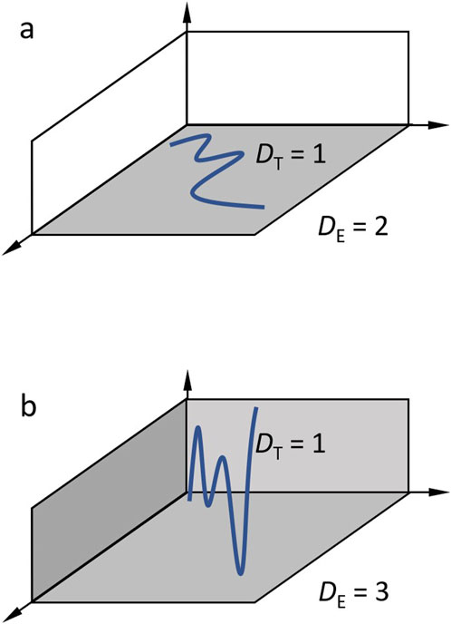
Figure 1. Illustration of topological and embedding dimension. (a) A topological 1D line is embedded in a 2D space. Fractal dimensions of the line can be between one and 2. (b) 3D embedding space. Fractal dimensions can be between 1 and 3.

4.5 Misconceptions and the role of prefractals

A crucial distinction in the fractal analysis is between true fractals and prefractals. Prefractals are approximations of fractals observed at finite iterations rather than infinitely repeating structures [207,222,223]. The Koch snowflake can serve as a useful test image for calibration but is not strictly fractal due to its finite nature when represented as an image due to the resolution limits of the computer [210]. When analyzing biological structures, using Euclidean reference objects (e.g., spheres, cubes) provides a baseline for comparison, but fractal-like forms require specialized methodologies. The challenge in fractal measurement lies in ensuring that the observed scaling relationship remains consistent across magnification levels. Statistical artifacts from image resolution, filtering, or incomplete iterations can lead to misclassification of biological structures as a fractal [131,156,157,224].

4.6 Self-similarity and biological forms

The broad use of the term self-similarity in biological contexts has contributed to confusion. In mathematical fractals, strict self-similarity means that identical patterns occur across all scales. However, biological systems exhibit statistical self-similarity, meaning that their scaling behavior follows probabilistic rather than deterministic patterns. This distinction is critical, as many biological forms including vascular networks and dendritic structures have been incorrectly classified as fractal when they merely exhibit scaling tendencies within a specific range [156]. A biological form should only be classified as fractal if its measured size follows a consistent power-law relationship across all scales, without a characteristic length limit. This is rarely the case in real-world biological systems [156,225]. How this may be addressed follows in the next section.

4.7 Defining surfaces, boundaries, and dimensional analysis

A critical consideration in 2D and 3D fractal analysis is the distinction between a surface, boundary, or perimeter in 2D and 3D structures and the determination and/or fixation of the topological dimension D_T [226,227]. A 2D boundary may represent the outermost silhouette of an object, as seen in fractal analyses of particle aggregates, whereas a 3D surface may include internal complexity, requiring different analysis techniques such as volume fractals and porous fractals [5,123,159,228–230]. For instance, silhouette-based fractal analysis of biological aggregates has been employed to quantify sludge morphology, but results can differ depending on whether the boundary or mass is analyzed. Estimates of silhouette boundaries tend to yield lower fractal dimensions compared to sectioned boundaries, highlighting the importance of defining measurement criteria [124,157,231]. Finally, any values of fractal D_F smaller than D_T are not reliable. And one must be aware of the actual embedding dimension D_E, because any values of D_F exceeding D_E are also not reliable.

5 Operationalizing fractal linguistics: a taxonomy and validation framework

To advance fractal linguistics from a conceptual critique to a practical, cross-disciplinary tool, a comprehensive taxonomy and validation framework designed to identify, classify, and resolve inconsistencies in fractal analysis is required. The proposed framework aims to standardize terminology, standardize methodologies without impeding new developments, and enhance interpretability across diverse fields of research. By providing a structured approach to fractal analysis, the framework promotes clearer communication, improves reproducibility, and enhances the translational potential of fractal measures in applications ranging from biomedical diagnostics to environmental modeling and seismic forecasting. The model framework includes semantic drift identification, methodological variability audit, and interpretation mapping. A prototypical application of the taxonomy is illustrated in Table 1.

Table 1

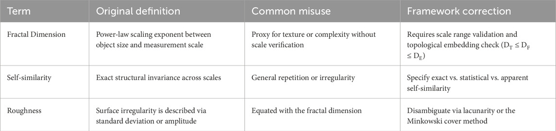
Table 1. Prototypical application of the fractal linguistics taxonomy to address semantic drift, methodological variability, and interpretation issues for key fractal terms.

Semantic drift occurs when fractal-related terms diverge from their original mathematical definitions as they are adopted across disciplines. This component of the taxonomy systematically traces and quantifies such divergences to restore terminological precision by identifying the definition of the term as established in mathematical fractal theory, documenting how the term is repurposed in applied disciplines, and developing qualitative or quantitative measures to assess the extent of drift. Practical implementation of semantic drift identification can be achieved through interdisciplinary workshops where domain experts and mathematicians collaboratively review terminology usage. Automated tools, such as natural language processing (NLP) algorithms, can scan literature databases to flag inconsistent definitions, enabling researchers to align their terminology with mathematical foundations. By clarifying terms like fractal dimension or self-similarity, this component addresses the communication gaps between mathematicians, who prioritize rigor, and applied scientists, who often adopt terms heuristically. See Table 2 for examples.

Table 2

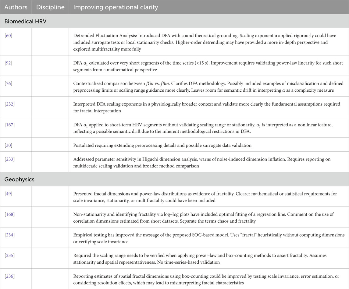
Table 2. Comparative Heart rate variability and geophysical fractal analysis studies.

Fractal analysis employs a variety of methods, such as box-counting, detrended fluctuation analysis (DFA), wavelet transforms, entropy measures, point processing and Higuchi’s algorithm, each with multiple implementation variants. These variants can lead to divergent outcomes, reducing comparability across studies. The methodological variability audit addresses this challenge through cataloging the specific fractal analysis method used, documenting variations in implementation, and conducting checks of robustness to evaluate how methodological choices affect results [237,238]. Practical implementation of the audit is already available and supported by open-access datasets and repository internet sites such as GitHub, which host computational tools and protocols for fractal analysis. Python or MATLAB libraries (e.g., https://www.mathworks.com/matlabcentral/fileexchange/71770-fractal-analysis-package; https://nolitia.com/; https://tsfel.readthedocs.io/en/latest/) can also provide reference implementations of DFA or box-counting, and include built-in sensitivity analysis modules to quantify the impact of parameter variations [239,240]. Researchers would be encouraged to report method-specific details in publications, adhering to a checklist derived from the audit framework [121,156,157]. This component ensures methodological transparency and reproducibility, which are critical for fields like biomedical engineering, where fractal analysis of heart rate variability (HRV) may use DFA with varying detrending orders. By standardizing reporting, the framework enables meta-analyses and cross-study comparisons, facilitating the development of universal benchmarks for fractal measures in physiological systems [241].

The last section of the framework addresses the interpretation of fractal analysis results, which often relies on implicit assumptions that may not hold across contexts, leading to overgeneralization or misinterpretations [242]. This component maps reported conclusions to their underlying assumptions and realigns them with the proposed framework to ensure validity. To achieve this, it is necessary to identify the reported findings of the study, explicitly articulating assumptions underpinning the interpretation, and adjusting interpretations based on validated assumptions. Practical implementation of interpretation mapping can be integrated into peer-review processes, where reviewers use standardized checklists to evaluate the alignment between claims and assumptions. Computational tools can assist by embedding diagnostic tests into fractal analysis pipelines, which provide researchers with feedback on the validity of their interpretations. This component has the potential to enhance the reliability of fractal-based conclusions in applied domains.

Table 1 demonstrates the application of the taxonomy to three key terms, highlighting their original definitions, common misuses, and proposed corrections. The table serves as a template for researchers to apply the framework to other terms and contexts.

The Supplementary Table 1 provides a more extended Glossary of terms that provides additional definitions, meant as a further guide to applying appropriate fractal terminology. The proposed taxonomy and validation framework enhances cross-disciplinary understanding and practical applications of fractal analysis by addressing semantic drift, methodological variability, and interpretation challenges. It ensures consistent use of terms like fractal dimension and self-similarity, improving communication across fields like biology, neuroscience, and environmental science. For example, it clarifies whether biological structures like vascular networks exhibit statistical or true fractality, ensures transparent documentation in EEG signal analysis, and validates scaling claims for coastal management. The framework aims to standardize reporting, enhance reproducibility, and support reliable applications, such as in biomedical diagnostics for diabetic retinopathy. It can also serve as an information tool, guiding non-specialists through fractal terminology and methods via workshops and resources. Future efforts should focus on developing computational tools, user-friendly software, interdisciplinary consensus guidelines, open-access educational materials, and validated data repositories to promote fractal literacy and reproducibility. This structured approach preserves mathematical rigor while enabling innovative solutions for complex natural and physiological systems.

5.1 Validation across disciplines: HRV and earthquake models

To validate the usefulness of this framework, we conducted a preliminary comparative analysis across two disciplines: biomedical signal processing, including heart rate variability (HRV), and geophysics, specifically earthquake models.

In HRV research, the term “fractal dimension” is often used interchangeably with measures of signal complexity, including Higuchi and Katz dimensions or DFA exponents, often without verifying scale-invariance or embedding dimension assumptions [31,60,111]. In contrast, geophysical models apply fractal statistics to seismic fault distributions and aftershock sequences, frequently assuming long-range correlations and multifractality, yet rarely assess stationarity or artifact influence [49,168,234].

By applying the proposed taxonomy, we reclassified methods and terminology in five key studies from each domain (Table 2). This revealed that in over 60% of HRV studies, reported scaling exponents reflected preprocessing artifacts or misapplication of DFA without proper data stationarity checks. Similarly, in geophysics, inconsistent use of the term “multifractal” emerged due to insufficient analysis of scale windows and spurious correlations introduced through detrending.

A review of the pivotal contributions to the field of fractal analysis, including the authors of Table 2 indicates the expanding interdisciplinary research in applying fractal-based analyses to natural and physiological systems (See also Supplementary Table 2). These studies have laid critical groundwork for modeling complexity, yet there is significant potential to advance fractal analysis methodology, reporting, and understanding of physical and biological systems by operationalizing a standardized framework that enhances clarity and precision. By adopting consistent reporting of scaling ranges, rigorous statistical validation of fractal dimensions, and clear differentiation between multifractality, long-range dependence, and stochastic variability, researchers can improve methodological robustness. Practical steps, such as integrating surrogate testing, resolution sensitivity analysis, and explicit log–log scaling diagnostics, will reinforce the fractal nature of the observed dynamics. Furthermore, refining the semantic precision of terms like “fractal” and “scale-free” by defining them through entropy-based metrics will lead to enhanced cross-disciplinary interpretability. These advancements will have an impact on translational opportunities that drive innovation in fields such as seismic forecasting, biomedical diagnostics, and networked system modeling, while promoting a unified and accessible fractal linguistics framework.

5.2 Key challenges in fractal linguistics

The variability in definitions across diverse fields includes terms like fractal dimension and self-similarity, which are used inconsistently and do not consider scale-invariance, the correct term to describe natural objects. Methodological uncertainty is perhaps the most challenging due to the plethora of computational methods available on the internet and in-house coding, which often generates fractal parameters without clarifying their theoretical foundations. Finally, overgeneralization, which addresses the assumption that all self-similar structures exhibit fractal properties, has resulted in the overuse of fractal models in biology and medicine.

Future research needs to consider prioritizing clearer definitions, interdisciplinary collaboration, and standardized methodologies in fractal-based studies to address these issues [180,202,243]. The current paper addresses some of these issues to fully realize the potential of fractal analysis in modeling complex systems. This requires greater emphasis on fractal analysis descriptions and definitions, especially in biological and clinical sciences. By establishing a linguistics model, which integrates correct descriptions of spatial, temporal, and multifractal approaches, the accuracy and reliability of fractal models can be improved [8,20,225]. The emerging field of fractal linguistics provides a framework for refining terminology, standardizing methodologies, and improving interdisciplinary discourse [11].

6 Conclusion

Fractal analysis is a versatile tool for quantifying the complexity of spatial structures and time series data. However, inconsistent terminology, methodological variability, and interpretation ambiguities reduce the effectiveness of the results and lead to semantic drift and communication barriers across multidisciplinary projects. This paper provides a critical commentary on the evolving usage of fractal and multifractal terminology in the analysis of complex systems and examines how foundational concepts such as fractional Brownian motion ($fBm$), self-affinity, and multifractality have been adapted, reinterpreted, and occasionally misapplied across disciplines. There is a growing divergence in how terms such as roughness, complexity, and scaling are understood in physics, finance, and biology. The oversimplification of the term roughness, which is a necessary but not sufficient condition for fractality, is often equated directly with the Hurst exponent and ignores the mathematical underpinning associated with scaling phenomena. A signal may be rough (e.g., non-differentiable or noisy) without being self-affine, multifractal, or long-range correlated. Clarifying this distinction is critical to avoid misleading interpretations of results. Multifractality is another ambiguous term if used in diverse contexts. As such, multifractality in econometrics may refer to time-varying Hölder exponents, while in statistical physics it implies a nonlinear $H\left(q\right)$ spectrum arising from multiplicative cascades. There is also a need to distinguish between true multifractality, characterized by nonlinear moment scaling and a broad multifractal spectrum $f\left(\alpha \right)$, and apparent multifractality, which may result from nonstationarity, fat-tailed distributions, or finite-size effects. This distinction is important for correctly describing underlying dynamical mechanisms. Throughout the manuscript, emphasis is placed on correctly applying contemporary descriptors, such as $nfBm$, $gfBm$, and $fLm$, that extend the original Mandelbrot and van Ness model and incorporate non-Gaussian, nonstationary, and generalized scaling behaviors. Correct use of these terms, which are found now in mathematical and physical sciences, is necessary to prevent terminological drift.

Ultimately, this work contributes to the metatheoretical architecture of fractal analysis. It seeks to foster terminological coherence and epistemological clarity in interdisciplinary research where fractals, scaling, and complexity are described. By tracing the genealogy of key concepts and explicitly differentiating between methods, phenomena, and metaphors, we hope to motivate more rigorous and reflexive applications of fractal models in empirical science. Future work should focus on expanding this framework through transdisciplinary reflection by researchers to use fractal language with both mathematical precision and conceptual transparency. This formalization is critical for improving accuracy and enhancing cross-disciplinary communication.

Author contributions

HJ: Conceptualization, Writing – original draft, Writing – review and editing. HA: Conceptualization, Writing – original draft, Writing – review and editing.

Funding

The author(s) declare that no financial support was received for the research and/or publication of this article.

Conflict of interest

The authors declare that the research was conducted in the absence of any commercial or financial relationships that could be construed as a potential conflict of interest.

The author(s) declared that they were an editorial board member of Frontiers, at the time of submission. This had no impact on the peer review process and the final decision.

Generative AI statement

The author(s) declare that no Generative AI was used in the creation of this manuscript.

Publisher’s note

All claims expressed in this article are solely those of the authors and do not necessarily represent those of their affiliated organizations, or those of the publisher, the editors and the reviewers. Any product that may be evaluated in this article, or claim that may be made by its manufacturer, is not guaranteed or endorsed by the publisher.

Supplementary material

The Supplementary Material for this article can be found online at: https://www.frontiersin.org/articles/10.3389/fphy.2025.1645620/full#supplementary-material

References

1. Hargittai I. Remembering Benoit Mandelbrot on his centennial – his fractal geometry changed our view of nature. Struct Chem (2024) 35(5):1657–61. doi:10.1007/s11224-024-02290-9

CrossRef Full Text | Google Scholar

2. Chen Y. Fractal modeling and fractal dimension description of urban morphology. Entropy (2020) 22(9):961. doi:10.3390/e22090961

PubMed Abstract | CrossRef Full Text | Google Scholar

3. Mandelbrot BB. The fractal geometry of nature. New York: Freeman and Co (1983).

Google Scholar

4. Taylor R, Spehar B, Hagerhall C, Van Donkelaar P. Perceptual and physiological responses to Jackson Pollock's fractals. Front Hum Neurosci (2011) 5:60. doi:10.3389/fnhum.2011.00060

PubMed Abstract | CrossRef Full Text | Google Scholar

5. Schroeder M. Fractals, chaos, power laws. New York: W. H. Freeman (1991).

Google Scholar

6. Falconer K. Fractal geometry: mathematical foundation and applications. 2 ed. London: John Wiley and Sons (2003).

Google Scholar

7. Wen R, Sinding-Larsen R. Uncertainty in fractal dimension estimated from power spectra and variograms. Math Geol (1997) 29(6):727–53. doi:10.1007/bf02768900

CrossRef Full Text | Google Scholar

8. Jelinek HF, Jones CL, Warfel MD. Is there meaning in fractal analyses? Compl Internat (1998) 6.

Google Scholar

9. Vicsek T. Fractal growth phenomena. 2 ed. Singapore: World Scientific (1992).

Google Scholar

10. Xue Y, Bogdan P. Reliable multifractal characterization of weighted complex networks: algorithms and implications. Sci Rep (2017) 7(1):7487. doi:10.1038/s41598-017-07209-5

PubMed Abstract | CrossRef Full Text | Google Scholar

11. Jelinek HF, Jones D, Warfel M, Lucas C, Depardieu C, Aurel G. Understanding fractal analysis? The case of fractal linguistics. ComPlexUs (2006) 9:66–73. doi:10.1159/000094189

CrossRef Full Text | Google Scholar

12. Korolj A, Wu HT, Radisic M. A healthy dose of chaos: using fractal frameworks for engineering higher-fidelity biomedical systems. Biomaterials (2019) 219:119363. doi:10.1016/j.biomaterials.2019.119363

PubMed Abstract | CrossRef Full Text | Google Scholar

13. Richardson LF. The problem of contiguity: an appendix o statistics of deadly quarrels. In: Q Wright, and CC Lienau, editors. Statistics fo deadly quarrels. Pittsburgh: Boxwood Press (1960). p. 139–87.

Google Scholar

14. Falconer K. Fractal geometry: mathematical foundations and applications. John Wiley and Sons (2013).

CrossRef Full Text | Google Scholar

15. Landini G. Fractals in microscopy. J Microsc (2011) 241(1):1–8. doi:10.1111/j.1365-2818.2010.03454.x

PubMed Abstract | CrossRef Full Text | Google Scholar

16. Katz MJ, George EB. Fractals and the analysis of growth paths. Bull Math Biol (1985) 47(2):273–86. doi:10.1007/bf02460036

PubMed Abstract | CrossRef Full Text | Google Scholar

17. Karperien AL, Jelinek HF. Box-counting fractal analysis: a primer for the clinician. In: A Di Ieva, editor. The fractal geometry of the brain. Cham: Springer International Publishing (2024). p. 15–55.

CrossRef Full Text | Google Scholar

18. Peptenatu D, Andronache I, Ahammer H, Radulovic M, Costanza J, Jelinek HF, et al. A new fractal index to classify forest disturbance and anthropogenic change. Landsc Ecol (2023) 38:1373–93. doi:10.1007/s10980-023-01640-y

CrossRef Full Text | Google Scholar

19. Chappard D, Legrand E, Haettich B, Chalès G, Auvinet B, Eschard JP, et al. Fractal dimension of trabecular bone: comparison of three histomorphometric computed techniques for measuring the architectural two-dimensional complexity. J Pathol (2001) 195(4):515–21. doi:10.1002/path.970

PubMed Abstract | CrossRef Full Text | Google Scholar

20. Jelinek HF, Tuladhar R, Culbreth G, Bohara G, Cornforth D, West BJ, et al. Diffusion entropy vs. Multiscale and Rényi entropy to detect progression of autonomic neuropathy. Front Physiol (2021) 11(1759):607324. doi:10.3389/fphys.2020.607324

PubMed Abstract | CrossRef Full Text | Google Scholar

21. Valencia JF, Porta A, Vallverdu M, Claria F, Baranowski R, Orlowska-Baranowska E, et al. Refined multiscale entropy: application to 24-h Holter recordings of heart period variability in healthy and aortic stenosis subjects. IEEE Trans Biomed Eng (2009) 56(9):2202–13. doi:10.1109/tbme.2009.2021986

PubMed Abstract | CrossRef Full Text | Google Scholar

22. Cornforth D, Jelinek HF, Tarvainen M. A comparison of nonlinear measures for the detection of cardiac autonomic neuropathy from heart rate variability. Entropy (2015) 17(3):1425–40. doi:10.3390/e17031425

CrossRef Full Text | Google Scholar

23. Tomashin A, Leonardi G, Wallot S. Four methods to distinguish between fractal dimensions in time series through recurrence quantification analysis. Entropy (Basel). (2022) 24(9):1314. doi:10.3390/e24091314

PubMed Abstract | CrossRef Full Text | Google Scholar

24. Ihlen EAF. Introduction to multifractal detrended fluctuation analysis in matlab. Front Physiol (2012) 3:141. doi:10.3389/fphys.2012.00141

PubMed Abstract | CrossRef Full Text | Google Scholar

25. Shi M, Shi Y, Lin Y, Qi X. Modified multiscale Renyi distribution entropy for short-term heart rate variability analysis. BMC Med Inform Decis Mak (2024) 24(1):346. doi:10.1186/s12911-024-02763-1

PubMed Abstract | CrossRef Full Text | Google Scholar

26. Mi Y, Lin A. Kernel based multiscale partial Renyi transfer entropy and its applications. Commun Nonlinear Sci Numer Simulation (2023) 119:107084. doi:10.1016/j.cnsns.2023.107084

CrossRef Full Text | Google Scholar

27. Nasrat SA, Mahmoodi K, Khandoker AH, Grigolini P, Jelinek HF. Multiscale diffusion entropy analysis for the detection of crucial events in cardiac pathology. Annu Int Conf IEEE Eng Med Biol Soc (2023) 2023:1–4. doi:10.1109/EMBC40787.2023.10340403

PubMed Abstract | CrossRef Full Text | Google Scholar

28. Faes L, Faes L, Porta A, Javorka M, Nollo G, Nollo G. Efficient computation of multiscale entropy over short biomedical time series based on linear state-space models. Complex (2017) 2017:–13. doi:10.1155/2017/1768264

CrossRef Full Text | Google Scholar

29. Baumert M, Javorka M, Seeck A, Faber R, Sanders P, Voss A. Multiscale entropy and detrended fluctuation analysis of QT interval and heart rate variability during normal pregnancy. Comput Biol Med (2012) 42(3):347–52. doi:10.1016/j.compbiomed.2011.03.019

PubMed Abstract | CrossRef Full Text | Google Scholar

30. Jelinek HF, Cornforth DJ, Tarvainen MP, Khalaf K. Investigation of linear and nonlinear properties of a heartbeat time series using multiscale Rényi entropy. Entropy (2019) 21(8):727. doi:10.3390/e21080727

PubMed Abstract | CrossRef Full Text | Google Scholar

31. Eke A, Herman P, Kocsis L, Kozak LR. Fractal characterization of complexity in temporal physiological signals. Physiol Meas (2002) 23(1):R1–38. doi:10.1088/0967-3334/23/1/201

PubMed Abstract | CrossRef Full Text | Google Scholar

32. Robles KE, Roberts M, Viengkham C, Smith JH, Rowland C, Moslehi S, et al. Aesthetics and psychological effects of fractal based design. Front Psychol (2021) 12–2021.

Google Scholar

33. Bies AJ, Blanc-Goldhammer DR, Boydston CR, Taylor RP, Sereno ME. Aesthetic responses to exact fractals driven by physical complexity. Front Hum Neurosci (2016) 10:210. doi:10.3389/fnhum.2016.00210

PubMed Abstract | CrossRef Full Text | Google Scholar

34. Danca M-F. Mandelbrot set as a particular julia set of fractional order, equipotential lines and external rays of Mandelbrot and julia sets of fractional order. Fractal Fractional (2024) 8(1):69. doi:10.3390/fractalfract8010069

CrossRef Full Text | Google Scholar

35. Andronache I, Liritzis I, Jelinek HF. Fractal algorithms and RGB image processing in scribal and ink identification on an 1819 secret initiation manuscript to the Philike Hetaereia. Sci Rep (2023) 13(1):1735. doi:10.1038/s41598-023-28005-4

PubMed Abstract | CrossRef Full Text | Google Scholar

36. Peptenatu D, Andronache I, Ahammer H, Taylor R, Liritzis I, Radulovic M, et al. Kolmogorov compression complexity may differentiate different schools of Orthodox iconography. Sci Rep (2022) 12(1):10743. doi:10.1038/s41598-022-12826-w

PubMed Abstract | CrossRef Full Text | Google Scholar

37. Patuano A, Lima MF. The fractal dimension of Islamic and Persian four-folding gardens. Hum Soc Sci Commun (2021) 8(1):86. doi:10.1057/s41599-021-00766-1

CrossRef Full Text | Google Scholar

38. Manera M. Perspectives on complexity, chaos and thermodynamics in environmental pathology. Int J Environ Res Public Health (2021) 18(11):5766. doi:10.3390/ijerph18115766

PubMed Abstract | CrossRef Full Text | Google Scholar

39. Watari S. Fractal dimensions of solar activity. Solar Phys (1995) 158(2):365–77. doi:10.1007/bf00795669

CrossRef Full Text | Google Scholar

40. Rypdal M, Rypdal K. Testing hypotheses about sun-climate complexity linking. Phys Rev Lett (2010) 104(12):128501. doi:10.1103/physrevlett.104.128501

PubMed Abstract | CrossRef Full Text | Google Scholar

41. Hampp F, Lindstedt RP. Fractal grid generated turbulence—a bridge to practical combustion applications. In: Y Sakai, and C Vassilicos, editors. Fractal flow design: how to design bespoke turbulence and why. Cham: Springer International Publishing (2016). p. 75–102.

CrossRef Full Text | Google Scholar

42. Bratanov V, Jenko F, Frey E. New class of turbulence in active fluids. Proc Natl Acad Sci U S A. (2015) 112(49):15048–53. doi:10.1073/pnas.1509304112

PubMed Abstract | CrossRef Full Text | Google Scholar

43. Chhabra AB, Meneveau C, Jensen RV, Sreenivasan KR. Direct determination of the f(alpha) singularity spectrum and its application to fully developed turbulence. Phys Rev A Gen Phys (1989) 40(9):5284–94. doi:10.1103/physreva.40.5284

PubMed Abstract | CrossRef Full Text | Google Scholar

44. Sreenivasan KR. Fractals and multifractals in fluid turbulence. Annu Rev Fluid Mech (1991) 23:539–604. doi:10.1146/annurev.fl.23.010191.002543

CrossRef Full Text | Google Scholar

45. Huang N, Han S, Zhang X, Wang G, Jiang Y. Effects of surface roughness and Reynolds number on the solute transport through three-dimensional rough-walled rock fractures under different flow regimes. Sci Rep (2024) 14(1):22452. doi:10.1038/s41598-024-73011-9

PubMed Abstract | CrossRef Full Text | Google Scholar

46. Dierking I. Fractal growth patterns in liquid crystals. Chem Phys Chem. (2001) 2(1):59–62. doi:10.1002/1439-7641(20010119)2:1<59::aid-cphc59>3.0.co;2-4

PubMed Abstract | CrossRef Full Text | Google Scholar

47. West BJ, Mudaliar S. Principles entailed by complexity, crucial events, and multifractal dimensionality. Entropy (2025) 27(3):241. doi:10.3390/e27030241

PubMed Abstract | CrossRef Full Text | Google Scholar

48. El-Nabulsi RA. A model for ice sheets and glaciers in fractal dimensions. Polar Sci (2025) 44:101171. doi:10.1016/j.polar.2025.101171

CrossRef Full Text | Google Scholar

49. Turcotte DL. Fractals and chaos in geology and geophysics. 2 ed. Cambridge: Cambridge University Press (1997).

Google Scholar

50. Venegas-Aravena P, Cordaro EG, Laroze D. Natural fractals as irreversible disorder: entropy approach from cracks in the semi brittle-ductile lithosphere and generalization. Entropy (2022) 24(10):1337. doi:10.3390/e24101337

PubMed Abstract | CrossRef Full Text | Google Scholar

51. Vahab S, Sankaran A. Multifractal applications in hydro-climatology: a comprehensive review of modern methods. Fractal and Fractional (2025) 9(1):27. doi:10.3390/fractalfract9010027

CrossRef Full Text | Google Scholar

52. Rodriguez-Iturbe I, Caylor KK, Rinaldo A. Metabolic principles of river basin organization. Proc Natl Acad Sci U S A. (2011) 108(29):11751–5. doi:10.1073/pnas.1107561108

PubMed Abstract | CrossRef Full Text | Google Scholar

53. Ma Y, He X, Wu R, Shen C. Spatial distribution of multi-fractal scaling behaviours of atmospheric XCO(2) concentration time series during 2010-2018 over China. Entropy (2022) 24(6):817. doi:10.3390/e24060817

PubMed Abstract | CrossRef Full Text | Google Scholar

54. Yuval BDM. Studying the time scale dependence of environmental variables predictability using fractal analysis. Environ Sci Technol (2010) 44(12):4629–34. doi:10.1021/es903495q

PubMed Abstract | CrossRef Full Text | Google Scholar

55. Katz RW, Brown BG. Extreme events in a changing climate: variability is more important than averages. Climat Change (1992) 21(3):289–302. doi:10.1007/bf00139728

CrossRef Full Text | Google Scholar

56. West BJ. Complexity synchronization in living matter: a mini review. Front Netw Physiol (2024) 4:1379892. doi:10.3389/fnetp.2024.1379892

PubMed Abstract | CrossRef Full Text | Google Scholar

57. Voss A, Schulz S, Schroeder R, Baumert M, Caminal P. Methods derived from nonlinear dynamics for analysing heart rate variability. Phil Trans Roy Soc A: math. Phys Eng Sci. (2009) 367(1887):277–96.

PubMed Abstract | CrossRef Full Text | Google Scholar

58. Mao X, Shang P, Wang J, Ma Y. Characterizing time series by extended complexity-entropy curves based on Tsallis, Rényi, and power spectral entropy. Chaos (2018) 28(11):113106. doi:10.1063/1.5038758

PubMed Abstract | CrossRef Full Text | Google Scholar

59. Ghosh D, Marwan N, Small M, Zhou C, Heitzig J, Koseska A, et al. Recent achievements in nonlinear dynamics, synchronization, and networks. Chaos (2024) 34(10):100401. doi:10.1063/5.0236801

PubMed Abstract | CrossRef Full Text | Google Scholar

60. Peng CK, Havlin S, Stanley HE, Goldberger AL. Quantification of scaling exponents and cross over phenomena in nonstationary heartbeat time series analysis. Chaos (1995) 5(1):82–7.

PubMed Abstract | CrossRef Full Text | Google Scholar

61. Ashkenazy Y, Ivanov PC, Havlin S, Peng CK, Yamamoto Y, Goldberger AL, et al. Decomposition of heartbeat time series: scaling analysis of the sign sequence. Com Cardiol (2000) 27:139–42.

PubMed Abstract | Google Scholar

62. MC Teich, SB Lowen, BM Jost, and K Vibe-Rheymer, editors. Heart rate variability: measures and models. New York: IEEE Press (2001).

Google Scholar

63. Wehler D, Jelinek HF, Gronau A, Wessel N, Kraemer JF, Krones R, et al. Reliability of heart-rate-variability features derived from ultra-short ECG recordings and their validity in the assessment of cardiac autonomic neuropathy. Biomed Sig Process Contr (2021) 68:102651. doi:10.1016/j.bspc.2021.102651

CrossRef Full Text | Google Scholar

64. Carricarte Naranjo C, Marras C, Visanji NP, Cornforth DJ, Sanchez-Rodriguez L, Schüle B, et al. Short-term deceleration capacity of heart rate: a sensitive marker of cardiac autonomic dysfunction in idiopathic Parkinson's disease. Clin Auton Res (2021) 31:729–36. doi:10.1007/s10286-021-00815-4

PubMed Abstract | CrossRef Full Text | Google Scholar

65. Marzbanrad F, Khandoker AH, Hambly BD, Ng E, Tamayo M, Lu Y, et al. Methodological comparisons of heart rate variability analysis in patients with type 2 diabetes and angiotensin converting enzyme polymorphism. IEEE J Biomed Health Inform (2016) 20(1):55–63. doi:10.1109/jbhi.2015.2480778

PubMed Abstract | CrossRef Full Text | Google Scholar

66. Khandoker AH, Weiss DN, Skinner JE, Anchin JM, Imam HM, Jelinek HF, et al. PD2i heart rate complexity measure can detect cardiac autonomic neuropathy: an alternative test to Ewing battery. In: Computing in cardiology. Hangzhou, China: IEEE Press (2011). p. 525–8.

Google Scholar

67. Oida E, Moritani T, Yamori Y. Tone-entropy analysis on cardiac recovery after dynamic exercise. J Appl Physiol (1997) 82(6):1794–801. doi:10.1152/jappl.1997.82.6.1794

PubMed Abstract | CrossRef Full Text | Google Scholar

68. Pawłowski R, Buszko K, Newton JL, Kujawski S, Zalewski P. Heart rate asymmetry analysis during head-up tilt test in healthy men. Front Physiol (2021) 12:657902. doi:10.3389/fphys.2021.657902

PubMed Abstract | CrossRef Full Text | Google Scholar

69. Tulppo MP, Mäkikallio TH, Seppänen T, Airaksinen JKE, Huikuri HV. Heart rate dynamics during accentuated sympathovagal interaction. Am J Physiol Heart Circ Physiol (1998) 274(3):H810–6. doi:10.1152/ajpheart.1998.274.3.H810

PubMed Abstract | CrossRef Full Text | Google Scholar

70. Brennan M, Kamen P, Palaniswami M. New insights into the relationship between Poincare plot geometry and linear measures of heart rate variability. Istanbul, Turkey: IEEE-EMBS (2001). Available online at: http://www.dtic.mil/cgi-bin/GetTRDoc?AD=ADA411633&Location=U2&doc=GetTRDoc.pdf.

CrossRef Full Text | Google Scholar

71. Karmakar CK, Khandoker AH, Gubbi J, Palaniswami M. Modified Ehler's index for improved detection of heart rate asymmetry on Poincaré Plot. Comp Cardiol (2009) 36:169–72.

Google Scholar

72. Karmakar CK, Khandoker A, Gubbi J, Palaniswami M. Complex correlation measure: a novel descriptor for Poincaré plot. Biomed Eng Online (2009) 8(17):17. doi:10.1186/1475-925x-8-17

PubMed Abstract | CrossRef Full Text | Google Scholar

73. Khan MSI, Jelinek HF. Point of care testing (POCT) in psychopathology using fractal analysis and Hilbert Huang Transform of electroencephalogram (EEG). In: A Di Ieva, editor. The fractal geometry of the brain. Cham: Springer International Publishing (2024). p. 693–715. doi:10.1007/978-3-031-47606-8_35

CrossRef Full Text | Google Scholar

74. Hurst HE. Long-term storage capacity of reservoirs. Trans Am Soc Civ Eng. (1951) 116:770–99. doi:10.1061/taceat.0006518

CrossRef Full Text | Google Scholar

75. Likens AD, Mangalam M, Wong AY, Charles AC, Mills C. Better than DFA? A Bayesian method for estimating the hurst exponent in behavioral sciences. ArXiv (2023):arXiv:2301.11262v1.

PubMed Abstract | Google Scholar

76. Eke A, Hermán P, Bassingthwaighte JB, Raymond GM, Percival DB, Cannon M, et al. Physiological time series: distinguishing fractal noises from motions. Eur J Physiol. (2000) 439(4):403–15. doi:10.1007/s004249900135

PubMed Abstract | CrossRef Full Text | Google Scholar

77. Schaefer A, Brach JS, Perera S, Sejdić E. A comparative analysis of spectral exponent estimation techniques for 1/f(β) processes with applications to the analysis of stride interval time series. J Neurosci Meth (2014) 222:118–30. doi:10.1016/j.jneumeth.2013.10.017

PubMed Abstract | CrossRef Full Text | Google Scholar

78. Delignières D, Torre K. Fractal dynamics of human gait: a reassessment of the 1996 data of Hausdorff et al. J Appl Physiol (2009) 106(4):1272–9.

PubMed Abstract | CrossRef Full Text | Google Scholar

79. Mandelbrot BB, van Ness JW. Fractional Brownian motions, fractional noises and applications. Siam Rev (1968) 10:422–37. doi:10.1137/1010093

CrossRef Full Text | Google Scholar

80. Sornette D. Critical phenomena in natural sciences. 2 ed. Heidelberg, Germany: Springer (2006). doi:10.1007/3-540-33182-4

CrossRef Full Text | Google Scholar

81. ben-Avraham D, Havlin S. Diffusion and reactions in fractals and disordered systems. Cambridge: Cambridge University Press (2000).

Google Scholar

82. Evangelista LR, Lenzi EK. An introduction to anomalous diffusion and relaxation. Cham, Switzerland: Springer (2023).

CrossRef Full Text | Google Scholar

83. West B, Deering W. Fractal physiology for physicists: Lévy statistics. Phys Rep (1994) 246:1–100. doi:10.1016/0370-1573(94)0005-7

CrossRef Full Text | Google Scholar

84. Metzler R, Klafter J. The random walk's guide to anomalous diffusion: a fractional dynamics approach. Phys Rep (2000) 339(1):1–77. doi:10.1016/s0370-1573(00)00070-3

CrossRef Full Text | Google Scholar

85. Laskin N, Lambadaris I, Harmantzis FC, Devetsikiotis M. Fractional Lévy motion and its application to network traffic modeling. Comput Netw (2002) 40(3):363–75.

CrossRef Full Text | Google Scholar

86. Nezhadhaghighi MG, Nakhlband A. Modeling and statistical analysis of non-Gaussian random fields with heavy-tailed distributions. Phys Rev E (2017) 95(4):042114. doi:10.1103/physreve.95.042114

PubMed Abstract | CrossRef Full Text | Google Scholar

87. Chorowski M, Gubiec T, Kutner R. Fundamental concepts. Anomalous stochastics: a comprehensive guide to multifractals. In: Random walks, and real-world applications. Cham: Springer Nature Switzerland (2025). p. 13–52.

Google Scholar

88. Peng CK, Buldyrev SV, Goldberger AL, Havlin S, Simons M, Stanley HE. Finite-size effects on long range correlations: implications for the analysis of DNA sequences. Phys Rev E (1993) 47(5):3730–3.

Google Scholar

89. Bassingthwaighte J, Raymond G. Evaluating rescaled range analysis for time series. Ann Biomed Eng (1994) 22:432–44. doi:10.1007/bf02368250

PubMed Abstract | CrossRef Full Text | Google Scholar

90. Raubitzek S, Corpaci L, Hofer R, Mallinger K. Scaling exponents of time series data: a machine learning approach. Entropy (2023) 25(12):1671. doi:10.3390/e25121671

PubMed Abstract | CrossRef Full Text | Google Scholar

91. Carpena P, Gómez-Extremera M, Bernaola-Galván PA. On the validity of detrended fluctuation analysis at short scales. Entropy (2021) 24(1):61. doi:10.3390/e24010061

PubMed Abstract | CrossRef Full Text | Google Scholar

92. Maestri R, Pinna GD, Porta A, Balocchi R, Sassi R, Signorini MG, et al. Assessing nonlinear properties of heart rate variability from short-term recordings: are these measurements reliable? Physiol Meas (2007) 28(9):1067–77. doi:10.1088/0967-3334/28/9/008

PubMed Abstract | CrossRef Full Text | Google Scholar

93. Fallahtafti F, Wurdeman SR, Yentes JM. Sampling rate influences the regularity analysis of temporal domain measures of walking more than spatial domain measures. Gait Posture (2021) 88:216–20. doi:10.1016/j.gaitpost.2021.05.031

PubMed Abstract | CrossRef Full Text | Google Scholar

94. Raffalt PC, McCamley J, Denton W, Yentes JM. Sampling frequency influences sample entropy of kinematics during walking. Med Biol Eng Comput (2019) 57(4):759–64. doi:10.1007/s11517-018-1920-2

PubMed Abstract | CrossRef Full Text | Google Scholar

95. Marmelat V, Duncan A, Meltz S. Effect of sampling frequency on fractal fluctuations during treadmill walking. PLoS One (2019) 14(11):e0218908. doi:10.1371/journal.pone.0218908

PubMed Abstract | CrossRef Full Text | Google Scholar

96. Zhang H, Zhou QQ, Chen H, Hu XQ, Li WG, Bai Y, et al. The applied principles of EEG analysis methods in neuroscience and clinical neurology. Mil Med Res (2023) 10(1):67. doi:10.1186/s40779-023-00502-7

PubMed Abstract | CrossRef Full Text | Google Scholar

97. Weron A, Burnecki K, Mercik S, Weron K. Complete description of all self-similar models driven by Lévy stable noise. Phys Rev E Stat Nonlin Soft Matter Phys (2005) 71(1 Pt 2):016113. doi:10.1103/physreve.71.016113

PubMed Abstract | CrossRef Full Text | Google Scholar

98. Muzy JF, Bacry E, Arneodo A. Multifractal formalism for fractal signals: the structure-function approach versus the wavelet-transform modulus-maxima method. Physical Review E, Stat Phys, Plasmas, Fluids, Related Interdiscipl Topics (1993) 47(2):875–84. doi:10.1103/physreve.47.875

PubMed Abstract | CrossRef Full Text | Google Scholar

99. Galaska R, Makowiec D, Dudkowska A, Koprowski A, Chlebus K, Wdowczyk-Szulc J, et al. Comparison of wavelet transform modulus maxima and multifractal detrended fluctuation analysis of heart rate in patients with systolic dysfunction of left ventricle. Ann Noninvasive Electrocardiol (2008) 13(2):155–64. doi:10.1111/j.1542-474x.2008.00215.x

PubMed Abstract | CrossRef Full Text | Google Scholar

100. Arnéodo A, Argoul F, Muzy JF, Tabard M, Bacry E. Beyond classical multifractal analysis using wavelets: uncovering a multiplicative process hidden in the geometrical complexity of diffusion limited aggregates. Fractals (1993) 1(3):629–49.

CrossRef Full Text | Google Scholar

101. Audit B, Bacry E, Muzy JF, Arneodo A. Wavelet-based estimators of scaling behavior. IEEE Trans Inform Theory (2002) 48(11):2938–54. doi:10.1109/tit.2002.802631

CrossRef Full Text | Google Scholar

102. Scafetta N, Hamilton P, Grigolini P. The thermodynamics of social processes: the teen birth phenomenon. Fractals (2001) 09(02):193–208. doi:10.48550/arXiv.cond-mat/0009020

CrossRef Full Text | Google Scholar

103. Scafetta N, West BJ. Multiresolution diffusion entropy analysis of time series: an application to births to teenagers in Texas. Chaos, Solitons and Fractals (2004) 20(1):179–85. doi:10.1016/s0960-0779(03)00442-9

CrossRef Full Text | Google Scholar

104. Scafetta N, Latora V, Grigolini P. Lévy scaling: the diffusion entropy analysis applied to DNA sequences. Phys Rev E (2002) 66:031906. doi:10.1103/physreve.66.031906

PubMed Abstract | CrossRef Full Text | Google Scholar

105. Scafetta N, Grigolini P. Scaling detection in time series: diffusion entropy analysis. Phys Rev E Stat Nonlin Soft Matter Phys (2002) 66(3 Pt 2A):036130. doi:10.1103/physreve.66.036130

PubMed Abstract | CrossRef Full Text | Google Scholar

106. Allegrini P, Benci V, Grigolini P, Hamilton P, Ignaccolo M, Menconi G, et al. Compression and diffusion: a joint approach to detect complexity. Chaos, Solitons and Fractals (2003) 15(3):517–35. doi:10.1016/s0960-0779(02)00136-4

CrossRef Full Text | Google Scholar

107. Kelty-Stephen DG, Mangalam M. Multifractal descriptors ergodically characterize non-ergodic multiplicative cascade processes. Physica A (2023) 617:128651. doi:10.1016/j.physa.2023.128651

CrossRef Full Text | Google Scholar

108. Grigolini P, Aquino G, Bologna M, Lukovic M, West BJ. A theory of 1/f noise in human cognition. Physica A (2009) 388:4192–204.

Google Scholar

109. Mahmoodi K, West BJ, Grigolini P. Self-organized temporal criticality: bottom-up resilience versus top-down vulnerability. Complexity (2018) 2018(1):8139058. doi:10.1155/2018/8139058

CrossRef Full Text | Google Scholar

110. Rafiei H, Akbarzadeh-T M-R. Understandable time frame-based biosignal processing. Biomedical Signal Processing and Control (2025) 103:107429. doi:10.1016/j.bspc.2024.107429

CrossRef Full Text | Google Scholar

111. West BJ. Colloquium: fractional calculus view of complexity: a tutorial. Rev Mod Phys. (2014) 86:1169–86. doi:10.1103/revmodphys.86.1169

CrossRef Full Text | Google Scholar

112. Valenza G, Citi L, Lanatá A, Scilingo EP, Barbieri R. Revealing real-time emotional responses: a personalized assessment based on heartbeat dynamics. Sci Rep (2014) 4:4998. doi:10.1038/srep04998

PubMed Abstract | CrossRef Full Text | Google Scholar

113. Lewis GF, Furman SA, McCool MF, Porges SW. Statistical strategies to quantify respiratory sinus arrhythmia: are commonly used metrics equivalent? Biol Psychol (2012) 89(2):349–64. doi:10.1016/j.biopsycho.2011.11.009

PubMed Abstract | CrossRef Full Text | Google Scholar

114. Goldberger AL, Peng C-K, Lipsitz LA. What is physiologic complexity and how does it change with aging and disease? Neurobiol Aging (2002) 23:23–6. doi:10.1016/s0197-4580(01)00266-4

PubMed Abstract | CrossRef Full Text | Google Scholar

115. Mansier P, Clairambault J, Charlotte N, Medigue C, Verneiren C, LePape G, et al. Linear and non-linear analyses of heart rate variability: a minireview. Cardiovac Res (1996) 31:371–9. doi:10.1016/s0008-6363(96)00009-0

PubMed Abstract | CrossRef Full Text | Google Scholar

116. Gowrisankar A, Banerjee S. Framework of fractals in data analysis: theory and interpretation. Eur Phys J Spec Top (2023) 232:965–7. doi:10.1140/epjs/s11734-023-00890-w

PubMed Abstract | CrossRef Full Text | Google Scholar

117. Goldberger AL, Amaral LAN, Hausdorff JM, Ivanov PC, Peng C-K, Stanley HE. Fractal dynamics in physiology: alterations with disease and aging. PNAS (2002) 99(90001):2466–72. doi:10.1073/pnas.012579499

PubMed Abstract | CrossRef Full Text | Google Scholar

118. Stoop R, Orlando G, Bufalo M, Della Rossa F. Exploiting deterministic features in apparently stochastic data. Sci Rep (2022) 12(1):19843. doi:10.1038/s41598-022-23212-x

PubMed Abstract | CrossRef Full Text | Google Scholar

119. Wagenmakers EJ, Farrell S, Ratcliff R. Estimation and interpretation of 1/fα noise in human cognition. Psychon Bull Rev (2004) 11(4):579–615. doi:10.3758/bf03196615

PubMed Abstract | CrossRef Full Text | Google Scholar

120. Jiang W, Liu Y, Wang J, Li R, Liu X, Zhang J. Problems of the grid size selection in differential box-counting (DBC) methods and an improvement strategy. Entropy (Basel). (2022) 24(7):977. doi:10.3390/e24070977

PubMed Abstract | CrossRef Full Text | Google Scholar

121. Fernandez E, Jelinek HF. Use of fractal theory in neuroscience: methods, advantages, and potential problems. Methods (2001) 24(4):309–21. doi:10.1006/meth.2001.1201

PubMed Abstract | CrossRef Full Text | Google Scholar

122. Smith JTG, Marks WB, Lange GD, Sheriff JWH, Neale EA. A fractal analysis of cell images. J Neurosci Methods (1989) 27(2):173–80. doi:10.1016/0165-0270(89)90100-3

PubMed Abstract | CrossRef Full Text | Google Scholar

123. Krohn S, Froeling M, Leemans A, Ostwald D, Villoslada P, Finke C, et al. Evaluation of the 3D fractal dimension as a marker of structural brain complexity in multiple-acquisition MRI. Hum Brain Mapp (2019) 40(11):3299–320. doi:10.1002/hbm.24599

PubMed Abstract | CrossRef Full Text | Google Scholar

124. Karperien AL, Jelinek HF. Morphology and fractal-based classifications of neurons and microglia in two and three dimensions. In: A Di Ieva, editor. The fractal geometry of the brain. Cham: Springer International Publishing (2024). p. 149–72.

Google Scholar

125. Ahammer H, Reiss MA, Hackhofer M, Andronache I, Radulovic M, Labra-Spröhnle F, et al. ComsystanJ: a collection of Fiji/ImageJ2 plugins for nonlinear and complexity analysis in 1D, 2D and 3D. PlosOne (2023) 18(10):e0292217. doi:10.1371/journal.pone.0292217

PubMed Abstract | CrossRef Full Text | Google Scholar

126. LA Donnan, M Paul, L Crowley, K Felesimo, and HF Jelinek, editors. Complexity and entropy of knee kinematics in a joint reposition test: effect of strapping and kinesiology taping. 2018 Digital Image Computing: techniques and Applications (DICTA). IEEE Press (2018).

Google Scholar

127. Caserta F, Eldred WD, Fernandez E, Hausman RE, Stanford LR, Bulderev SV, et al. Determination of fractal dimension of physiologically characterized neurons in two and three dimensions. J Neurosci Meth (1995) 56:133–44. doi:10.1016/0165-0270(94)00115-w

PubMed Abstract | CrossRef Full Text | Google Scholar

128. Grela J, Drogosz Z, Janarek J, Ochab JK, Cifre I, Gudowska-Nowak E, et al. Using space-filling curves and fractals to reveal spatial and temporal patterns in neuroimaging data. J Neural Eng (2025) 22(1):016016. doi:10.1088/1741-2552/ada705

PubMed Abstract | CrossRef Full Text | Google Scholar

129. Murray JD. Use and abuse of fractal theory in neuroscience. J Comp Neurol (1995) 361:369–71. doi:10.1002/cne.903610302

PubMed Abstract | CrossRef Full Text | Google Scholar

130. Xu HHA, Yang XIA. Fractality and the law of the wall. Phys Rev E (2018) 97(5-1):053110. doi:10.1103/physreve.97.053110

PubMed Abstract | CrossRef Full Text | Google Scholar

131. Jin Y, Wu Y, Li H, Zhao M, Pan J. Definition of fractal topography to essential understanding of scale-invariance. Sci Rep (2017) 7:46672. doi:10.1038/srep46672

PubMed Abstract | CrossRef Full Text | Google Scholar

132. Karperien AL, Jelinek HF. Fractal, multifractal, and lacunarity analysis of microglia in tissue engineering. Front Bioeng Biotechnol (2015) 3(51):51. doi:10.3389/fbioe.2015.00051

PubMed Abstract | CrossRef Full Text | Google Scholar

133. Landini G, Murray PI, Misson GP. Local connected fractal dimensions and lacunarity analyses of 60 degrees fluorescein angiograms. Invest Ophthalmol Vis Sci. (1995) 36:2749–55.

PubMed Abstract | Google Scholar

134. Cornforth D, Tarvainen M, Jelinek HF. How to calculate renyi entropy from heart rate variability, and why it matters for detecting cardiac autonomic neuropathy. Front Bioeng Biotech (2014) 2:34. doi:10.3389/fbioe.2014.00034

PubMed Abstract | CrossRef Full Text | Google Scholar

135. Costa M, Goldberger AL, Peng C-K. Multiscale entropy analysis of biological signals. Phys Rev E (2005) 71:021906. doi:10.1103/physreve.71.021906

PubMed Abstract | CrossRef Full Text | Google Scholar

136. Nasrat S, Prasad R, Dimassi Z, Alefishat E, Khandoker A, Jelinek HF. Multiscaled crucial events complexity analysis of heart rate signals during Tibetan singing bowls meditation. In: Esgco 2024. Zaragoza, Spain: IEEE Press (2024).

Google Scholar

137. Theiler J, Eubank S, Longtin A, Galdrikian B, Doyne Farmer J. Testing for nonlinearity in time series: the method of surrogate data. Physica D: Nonlinear Phenomena (1992) 58(1):77–94. doi:10.1016/0167-2789(92)90102-s

CrossRef Full Text | Google Scholar

138. Grech D, Pamuła G. The local Hurst exponent of the financial time series in the vicinity of crashes on the Polish stock exchange market. Physica A (2008) 387:4299–308. doi:10.1016/j.physa.2008.02.007

CrossRef Full Text | Google Scholar

139. Schreiber T, Schmitz A. Improved surrogate data for nonlinearity tests. Phys Rev Lett (1996) 77:635–8. doi:10.1103/physrevlett.77.635

PubMed Abstract | CrossRef Full Text | Google Scholar

140. Kantelhardt JW, Zschiegner SA, Koscielny-Bunde E, Havlin S, Bunde A, Stanley HE. Multifractal detrended fluctuation analysis of nonstationary time series. Physica A (2002) 316(1):87–114. doi:10.1016/s0378-4371(02)01383-3

CrossRef Full Text | Google Scholar

141. Vacha L, Barunik J. Co-movement of energy commodities revisited: evidence from wavelet coherence analysis. Energ Econ (2012) 34(1):241–7. doi:10.1016/j.eneco.2011.10.007

CrossRef Full Text | Google Scholar

142. Calvet L, Fisher A. Multifractality in asset returns: theory and evidence. Rev Econ Stat (2002) 84(3):381–406. doi:10.1162/003465302320259420

CrossRef Full Text | Google Scholar

143. Ivanov P, Amaral LAN, Goldberger AL, Havlin S, Rosenblum M, Struzik ZR, et al. Multifractality in human heartbeat dynamics. Nature (1999) 399:461–5. doi:10.1038/20924

PubMed Abstract | CrossRef Full Text | Google Scholar

144. Stanley HE, Amaral LAN, Goldberger AL, Havlin S, Ivanov PC, Peng CK. Statistical physics and physiology: monofractal and multifractal approaches. Phys A (1999) 270:309–24. doi:10.1016/s0378-4371(99)00230-7

PubMed Abstract | CrossRef Full Text | Google Scholar

145. Kantz H. Nonlinear time series analysis — potentials and limitations. Berlin, Heidelberg: Springer Berlin Heidelberg (1996). p. 213–28.

CrossRef Full Text | Google Scholar

146. Feder J. Fractals. New York: Plenum Press (1988).

Google Scholar

147. Halsey TC, Jensen MH, Kadanoff LP, Procaccia I, Shraiman BI. Fractal measures and their singularities: the characterization of strange sets. Phys Rev A (1986) 33(2):1141–51. doi:10.1103/physreva.33.1141

PubMed Abstract | CrossRef Full Text | Google Scholar

148. Alvarez-Ramirez J, Alvarez J, Rodriguez E. Short-term predictability of crude oil markets: a detrended fluctuation analysis approach. Energ Econ (2008) 30(5):2645–56. doi:10.1016/j.eneco.2008.05.006

CrossRef Full Text | Google Scholar

149. Serinaldi F. Use and misuse of some Hurst parameter estimators applied to stationary and non-stationary financial time series. Physica A (2010) 389:2770–81. doi:10.1016/j.physa.2010.02.044

CrossRef Full Text | Google Scholar

150. Mahmoodi K, West BJ, Grigolini P. Self-organizing complex networks: individual versus global rules. Front Physiol (2017) 8:478. doi:10.3389/fphys.2017.00478

PubMed Abstract | CrossRef Full Text | Google Scholar

151. Haken H. Synergetics: an introduction. 3 ed. Heidelberg: Springer Verlag (1983).

Google Scholar

152. Jaeger HM, Liu AJ (2010). Far-from-equilibrium physics: an overview. arXiv preprint:10094874.

Google Scholar

153. Barunik J, Kristoufek L. On Hurst exponent estimation under heavy-tailed distributions. Physica A (2010) 389:3844–55. doi:10.1016/j.physa.2010.05.025

CrossRef Full Text | Google Scholar

154. Di Matteo T, Aste T, Dacorogna MM. Long-term memories of developed and emerging markets: using the scaling analysis to characterize their stage of development. J Banking Finance (2005) 29(4):827–51. doi:10.1016/j.jbankfin.2004.08.004

CrossRef Full Text | Google Scholar

155. Schizas I, Sullivan S, Kerick SE, Mahmoodi K, Bradford JC, Boothe DL, et al. (2024).Complexity synchronization analysis of neurophysiological data: theory and methods. arXiv preprint arXiv:241114602.

Google Scholar

156. Jelinek HF, Elston GN, Zietsch B. Fractal analysis: pitfalls and revelations in neuroscience. In: GA Losa, ER Weibel, and TF Nonnenmacher, editors. Fractals in biology and medicine, IV. Lucarno, Switzerland (2005). p. 85–94. Birkäuser Verlag. doi:10.1007/3-7643-7412-8_8

CrossRef Full Text | Google Scholar

157. Jelinek HF, Fernández E. Neurons and fractals: how reliable and useful are calculations of fractal dimension? J Neurosci Meth (1998) 81:9–18.

PubMed Abstract | CrossRef Full Text | Google Scholar

158. Dollinger JW, R M, Nonnenmacher TF. Bi-asymptotic fractals: fractals between lower and upper bounds. Journal of Physics A: Math Gen. (1998) 31:3839–47.

Google Scholar

159. Rigaut JP. An empirical formulation relating boundary lengths to resolution in specimens showing 'non-ideally fractal' dimensions. J Microsc (1984) 133:41–54. doi:10.1111/j.1365-2818.1984.tb00461.x

CrossRef Full Text | Google Scholar

160. Costa LF, Manoel ETM, Faucereau F, Chelly J, van Pelt J, Ramakers G. A shape analysis framework for neuromorphometry. Network: Comput Neural Syst (2002) 13:283–310. doi:10.1088/0954-898x_13_3_303

PubMed Abstract | CrossRef Full Text | Google Scholar

161. Zhao S, Jiang Y, He W, Mei Y, Xie X, Wan S. Detrended fluctuation analysis based on best-fit polynomial. Front Environ Sci. (2022) 10:1054689. doi:10.3389/fenvs.2022.1054689

CrossRef Full Text | Google Scholar

162. Silva RP, Zarpelão BB, Cano A, Junior SB. Time series segmentation based on stationarity analysis to improve new samples prediction. Sensors (2021) 21(21):7333. doi:10.3390/s21217333

PubMed Abstract | CrossRef Full Text | Google Scholar

163. Pinto H, Lazic I, Antonacci Y, Pernice R, Gu D, Barà C, et al. Testing dynamic correlations and nonlinearity in bivariate time series through information measures and surrogate data analysis. Front Netw Physiol (2024) 4:1385421. doi:10.3389/fnetp.2024.1385421

PubMed Abstract | CrossRef Full Text | Google Scholar

164. Saleem S, Khandoker AH, Alkhodari M, Hadjileontiadis LJ, Jelinek HF. A two-step pre-processing tool to remove Gaussian and ectopic noise for heart rate variability analysis. Sci Rep (2022) 12(1):18396. doi:10.1038/s41598-022-21776-2

PubMed Abstract | CrossRef Full Text | Google Scholar

165. Gu Z, Zarubin V, Martsberger C. The effectiveness of time domain and nonlinear heart rate variability metrics in ultra-short time series. Physiol Rep (2023) 11(22):e15863. doi:10.14814/phy2.15863

PubMed Abstract | CrossRef Full Text | Google Scholar

166. Shaffer F, Ginsberg JP. An overview of heart rate variability metrics and norms. Front Publ Hlth. (2017) 5:258. doi:10.3389/fpubh.2017.00258

PubMed Abstract | CrossRef Full Text | Google Scholar

167. Brennan M, Palaniswami M, Kamen P. Do existing methods of Poincaré plot geometry reflect nonlinear features of heart rate variability? IEEE Trans Biomed Eng (2001) 48(11):1342–7.

PubMed Abstract | CrossRef Full Text | Google Scholar

168. Goltz C. Fractal and chaotic properties of earthquakes. Berlin: Springer Verlag (1997).

Google Scholar

169. Zhang S, Fang W. Multifractal behaviors of stock indices and their ability to improve forecasting in a volatility clustering period. Entropy (2021) 23(8):1018. doi:10.3390/e23081018

PubMed Abstract | CrossRef Full Text | Google Scholar

170. de Melo Barros Junior PR, Bunge KL, Serravalle Reis Rodrigues VH, Ferreira SMT, dos Santos Marinho EB, Lima de Jesus SJL. Multi-fractal detrended cross-correlation heatmaps for time series analysis. Sci Rep (2022) 12(1):21655. doi:10.1038/s41598-022-26207-w

PubMed Abstract | CrossRef Full Text | Google Scholar

171. Nordbeck PC, Andrade V, Silva PL, Kuznetsov NA. DFA as a window into postural dynamics supporting task performance: does choice of step size matter? Front Netw Physiol (2023) 3:1233894. doi:10.3389/fnetp.2023.1233894

PubMed Abstract | CrossRef Full Text | Google Scholar

172. Zunino L, Tabak BM, Figliola A, Pérez DG, Garavaglia M, Rosso OA. A multifractal approach for stock market inefficiency. Physica A: Stat Mechan Applicat (2008) 387(26):6558–66. doi:10.1016/j.physa.2008.08.028

CrossRef Full Text | Google Scholar

173. Barnsley MF. Fractals everywhere. Academic Press (2014).

Google Scholar

174. Golmankhaneh AK, Welch K, Tunç C, Gasimov YS. Classical mechanics on fractal curves. Eur Phys J Spec Top (2023) 232(7):991–9.

CrossRef Full Text | Google Scholar

175. Glenny RW, Robertson HT. Fractal modeling of pulmonary blood flow heterogeneity. J Appl Physiol (1991) 70(3):1024–30. doi:10.1152/jappl.1991.70.3.1024

PubMed Abstract | CrossRef Full Text | Google Scholar

176. West BJ. The Fractal tapestry of life: a review of fractal physiology. Nonlin Dynam Psychol Life Sci. (2021) 25(3):261–96.

PubMed Abstract | Google Scholar

177. Sandau K, Kurz H. Measuring fractal dimension and complexity - an alternative approach with an application. J Microscop (1997) 186(2):164–76. doi:10.1046/j.1365-2818.1997.1270685.x

PubMed Abstract | CrossRef Full Text | Google Scholar

178. Jaquette J, Schweinhart B. Fractal dimension estimation with persistent homology: a comparative study. Commun Nonlinear Sci Numer Simul (2020) 84:105163. doi:10.1016/j.cnsns.2019.105163

PubMed Abstract | CrossRef Full Text | Google Scholar

179. West BJ. Where medicine went wrong: rediscovering the path to complexity: World Scientific (2006). 352. doi:10.1142/6175

CrossRef Full Text | Google Scholar

180. Bassingthwaighte JB, Liebovitch LS, West BJ. Fractal physiology. New York: Oxford University Press (1994). p. 364.

Google Scholar

181. Mandelbrot BB. Fractals, lacunarity and how it can be tuned and measured. In: TF Nonnenmacher, GA Losa, and ER Weibel, editors. Fractals in biology and medicine. Boston: Birkhäuser Verlag (1993). p. 21–8.

Google Scholar

182. Vicsek M, Vicsek T. Aggregation models of fractal growth. CWI Quart. (1997) 10(2):153–78.

Google Scholar

183. Bohara G, Lambert D, West BJ, Grigolini P. Crucial events, randomness, and multifractality in heartbeats. Phys Rev E (2017) 96(6-1):062216. doi:10.1103/physreve.96.062216

PubMed Abstract | CrossRef Full Text | Google Scholar

184. Struzik ZR. Fractals under the microscope or reaching beyond the dimensional formalism of fractals with the wavelet transform. CWI Quart (1997) 10(2):109–51.

Google Scholar

185. Ristanović D, Stevanovic BD, Milošević NT, Grgurevic M, Stulic V, Stulić V. Fractal and nonfractal analysis of cell images: comparison and application to neuronal dendritic arborization. Biol Cybern (2002) 87:278–88. doi:10.1007/s00422-002-0342-1

PubMed Abstract | CrossRef Full Text | Google Scholar

186. Baumert M, Brechtel LM, Lock J, Voss A, Abbott D. Scaling graphs of heart rate time series in athletes demonstrating the VLF, LF and HF regions. Physiol Meas (2006) 27:N35–N9. doi:10.1088/0967-3334/27/9/n01

PubMed Abstract | CrossRef Full Text | Google Scholar

187. Milošević NT, Rajković N, Jelinek HF. In: E Aguilar, editor. Fractal and multifractal analysis of two dimensional images of the retinopathy of prematurity: morphologic parameters and classification. Nova Publishers (2015).

Google Scholar

188. Masters BR. Fractal analysis of the vascular tree in the human retina. Ann Rev Biomed Eng (2004) 6:427–52. doi:10.1146/annurev.bioeng.6.040803.140100

PubMed Abstract | CrossRef Full Text | Google Scholar

189. Karperien AL, Jelinek HF. ImageJ in computational fractal-based neuroscience: pattern extraction and translational research. In: A Di Ieva, editor. The fractal geometry of the brain. Cham: Springer International Publishing (2024). p. 795–814.

CrossRef Full Text | Google Scholar

190. Jelinek HF, Elston GN. Dendritic branching of pyramidal cells in the visual cortex of the nocturanal owl monkey: a fractal analysis. Fractals (2004) 11(4):391–6.

Google Scholar

191. A di Ieva, editor. The fractal geometry of the brain. 2 ed. Berlin: Springer Verlag (2024).

Google Scholar

192. Andronache I. Analysis of forest fragmentation and connectivity using fractal dimension and succolarity. Land (2024) 13(2):138. doi:10.3390/land13020138

CrossRef Full Text | Google Scholar

193. Robles KE, Roberts M, Viengkham C, Smith JH, Rowland C, Moslehi S, et al. Aesthetics and psychological effects of fractal based design. Front Psychol (2021) 12:699962. doi:10.3389/fpsyg.2021.699962

PubMed Abstract | CrossRef Full Text | Google Scholar

194. Cerasa A. Fractals in neuropsychology and cognitive neuroscience. In: A Di Ieva, editor. The fractal geometry of the brain. Cham: Springer International Publishing (2024). p. 761–78.

Google Scholar

195. Tenti JM, Hernández Guiance SN, Irurzun IM. Fractal dimension of diffusion-limited aggregation clusters grown on spherical surfaces. Phys Rev E (2021) 103(1-1):012138. doi:10.1103/physreve.103.012138

PubMed Abstract | CrossRef Full Text | Google Scholar

196. Grebenkov DS, Beliaev D. How anisotropy beats fractality in two-dimensional on-lattice diffusion-limited-aggregation growth. Phys Rev E (2017) 96(4-1):042159. doi:10.1103/physreve.96.042159

PubMed Abstract | CrossRef Full Text | Google Scholar

197. Wu H, Lattuada M, Morbidelli M. Dependence of fractal dimension of DLCA clusters on size of primary particles. Adv Colloid Interface Sci (2013) 195-196:41–9. doi:10.1016/j.cis.2013.04.001

PubMed Abstract | CrossRef Full Text | Google Scholar

198. Procaccia EB, Procaccia I. Dimension of diffusion-limited aggregates grown on a line. Phys Rev E (2021) 103(2):L020101. doi:10.1103/physreve.103.l020101

PubMed Abstract | CrossRef Full Text | Google Scholar

199. Ghosh A, Batabyal R, Das GP, Dev BN. An extended fractal growth regime in the diffusion limited aggregation including edge diffusion. AIP Adv (2016) 6(1):015301. doi:10.1063/1.4939635

CrossRef Full Text | Google Scholar

200. Vicsek T, Family F, Meakin P. Multifractal geometry of diffusion-limited aggregates. Europhys Lett (1990) 12(3):217–22. doi:10.1209/0295-5075/12/3/005

CrossRef Full Text | Google Scholar

201. Polimeno M, Kim C, Blanchette F. Toward a realistic model of diffusion-limited aggregation: rotation, size-dependent diffusivities, and settling. ACS Omega (2022) 7(45):40826–35. doi:10.1021/acsomega.2c03547

PubMed Abstract | CrossRef Full Text | Google Scholar

202. Song J, Wang B, Jiang Q, Hao X. Exploring the role of fractal geometry in engineering image processing based on similarity and symmetry: a review. Symmetry (2024) 16(12):1658. doi:10.3390/sym16121658

CrossRef Full Text | Google Scholar

203. Tuladhar R, Bohara G, Grigolini P, West BJ. Meditation-induced coherence and crucial events. Front Physiol (2018) 9(626):626. doi:10.3389/fphys.2018.00626

PubMed Abstract | CrossRef Full Text | Google Scholar

204. Castillo O, Melin P. A new fuzzy fractal control approach of non-linear dynamic systems: the case of controlling the COVID-19 pandemics. Chaos Solitons Fractals (2021) 151:111250. doi:10.1016/j.chaos.2021.111250

PubMed Abstract | CrossRef Full Text | Google Scholar

205. Zueva MV. Fractality of sensations and the brain health: the theory linking neurodegenerative disorder with distortion of spatial and temporal scale-invariance and fractal complexity of the visible world. Front Aging Neurosci (2015) 7:135. doi:10.3389/fnagi.2015.00135

PubMed Abstract | CrossRef Full Text | Google Scholar

206. West BJ, Deering W. Fractal physiology for physicists: Lévy statistics. Phys Rep (1994) 246(1):1–100. doi:10.1016/0370-1573(94)00055-7

CrossRef Full Text | Google Scholar

207. Czyża S, Szuniewicz K, Cieślak I, Biłozor A, Bajerowski T. An analysis of the spatial development of European cities based on their geometry and the CORINE land cover (CLC) database. Int J Environ Res Public Health (2023) 20(3):2049. doi:10.3390/ijerph20032049

PubMed Abstract | CrossRef Full Text | Google Scholar

208. Gadelmawla ES, Koura M, Maksoud T, Elewa I, Soliman H. Roughness parameters. J Mater Process Technol (2002) 123:133–45. doi:10.1016/s0924-0136(02)00060-2

CrossRef Full Text | Google Scholar

209. Parsons DF, Walsh RB, Craig VS. Surface forces: surface roughness in theory and experiment. J Chem Phys (2014) 140(16):164701. doi:10.1063/1.4871412

PubMed Abstract | CrossRef Full Text | Google Scholar

210. Peitgen H-O, Jürgens H, Saupe D. Fractals for the classroom. Berlin: Springer-Verlag (1992).

Google Scholar

211. HR Bittner, and M Sernetz, editors. Selfsimilarity within limits: description with the log-logistic function. Lisboa (1990). p. 86.

Google Scholar

212. Losa G, Ristanović D, Ristanović D, Zaletel I, Beltraminelli S. From fractal geometry to fractal analysis. Appl Math (2016) 216(7):346–54. doi:10.4236/am.2016.74032

CrossRef Full Text | Google Scholar

213. Panico J, Sterling P. Retinal neurons and vessels are not fractal but space-filling. J Comp Neurol (1995) 361:479–90. doi:10.1002/cne.903610311

PubMed Abstract | CrossRef Full Text | Google Scholar

214. Schulz S, Schumann A, Bär K-J, Haueisen J, Seifert G, Voss A. A new directionality index based on high-resolution joint symbolic dynamics to assess information transfer in multivariate networks. Front Neurosci (2025) 19:1504161. doi:10.3389/fnins.2025.1504161

PubMed Abstract | CrossRef Full Text | Google Scholar

215. Lopes R. Multifractal analysis in neuroimaging. In: A Di Ieva, editor. The fractal geometry of the brain. Cham: Springer International Publishing (2024). p. 79–93.

CrossRef Full Text | Google Scholar

216. Nelson TR, West BJ, Goldberger AL. The fractal lung: universal and species-related scaling patterns. Experientia (1990) 46:251–4. doi:10.1007/bf01951755

PubMed Abstract | CrossRef Full Text | Google Scholar

217. Masters BR, Sernetz M, Wlczek P. Image analysis of human retinal blood vessels and their characterisation as fractals. ACTA Stereol (1992) 11(Suppl. 1):355–60.

Google Scholar

218. Sernetz M, Justen M, Jestczemski F. Dispersive fractal characterization of kidney arteries by three-dimensional mass-radius analysis. Fractals (1995) 3(4):879–91. doi:10.1142/s0218348x95000771

CrossRef Full Text | Google Scholar

219. D Cornforth, and HF Jelinek, editors. Automated classification of dementia subtypes from post-mortem cortex images. AI2005: advances in artificial intelligence. Sydney, Australia: Springer Verlag (2005). conference paper.

Google Scholar

220. Helmberger M, Pienn M, Urschler M, Kullnig P, Stollberger R, Kovacs G, et al. Quantification of tortuosity and fractal dimension of the lung vessels in pulmonary hypertension patients. Plos One (2014) 9(1):e87515. doi:10.1371/journal.pone.0087515

PubMed Abstract | CrossRef Full Text | Google Scholar

221. Jestczemski FHB, Sernetz M. Comparison of the surface dimension and the mass dimension of blood vessel systems. Fractals (1996) 4(2):123–32.

Google Scholar

222. Kochkarov R, Kochkarov A. Introduction to the class of prefractal graphs. Mathematics (2022) 10(14):2500. doi:10.3390/math10142500

CrossRef Full Text | Google Scholar

223. Chen Y. The solutions to the uncertainty problem of urban fractal dimension calculation. Entropy (2019) 21(5):453. doi:10.3390/e21050453

PubMed Abstract | CrossRef Full Text | Google Scholar

224. Curtin L. Fractal-based morphometrics of glioblastoma. Adv Neurobiol (2024) 36. 545–55. doi:10.1007/978-3-031-47606-8_28

PubMed Abstract | CrossRef Full Text | Google Scholar

225. Fernández E, Eldred WD, Ammermuller J, Block A, Von Bloh W, Kolb H. Complexity and scaling properties of amacrine, ganglion, horizontal, and bipoloar cells in the turtle retina. J Comp Neurol (1994) 347:397–408.

PubMed Abstract | CrossRef Full Text | Google Scholar

226. Ruiz de Miras J, Navas J, Villoslada P, Esteban FJ. UJA-3DFD: a program to compute the 3D fractal dimension from MRI data. Comput Methods Programs Biomed (2011) 104(3):452–60. doi:10.1016/j.cmpb.2010.08.015

PubMed Abstract | CrossRef Full Text | Google Scholar

227. Zhang L, Liu JZ, Dean D, Sahgal V, Yue GH. A three-dimensional fractal analysis method for quantifying white matter structure in human brain. J Neurosci Meth. (2006) 150(2):242–53. doi:10.1016/j.jneumeth.2005.06.021

PubMed Abstract | CrossRef Full Text | Google Scholar

228. Goñi J, Sporns O, Cheng H, Aznárez-Sanado M, Wang Y, Josa S, et al. Robust estimation of fractal measures for characterizing the structural complexity of the human brain: optimization and reproducibility. Neuroimage. (2013) 83:646–57. doi:10.1016/j.neuroimage.2013.06.072

PubMed Abstract | CrossRef Full Text | Google Scholar

229. Ahammer H, DeVaney TT. The influence of edge detection algorithms on the estimation of the fractal dimension of binary digital images. Chaos (2004) 14(1):183–8. doi:10.1063/1.1638947

PubMed Abstract | CrossRef Full Text | Google Scholar

230. Sendker FL, Lo YK, Heimerl T, Bohn S, Persson LJ, Mais C-N, et al. Emergence of fractal geometries in the evolution of a metabolic enzyme. Nature (2024) 628(8009):894–900. doi:10.1038/s41586-024-07287-2

PubMed Abstract | CrossRef Full Text | Google Scholar

231. Keller JM, Crownover RM, Chen RY. Characteristics of natural scenes related to the fractal dimension. IEEE Trans Pattern Anal Mach Intell (1987) 9(5):621–7. doi:10.1109/tpami.1987.4767956

PubMed Abstract | CrossRef Full Text | Google Scholar

232. DL Turcotte, editor. Scale invariance. Fractals and chaos in geology and geophysics, 2. Cambridge: Cambridge University Press (1997). p. 1–5.

Google Scholar

233. Müller W, Jung A, Ahammer H. Advantages and problems of nonlinear methods applied to analyze physiological time signals: human balance control as an example. Sci Rep (2017) 7(1):2464. doi:10.1038/s41598-017-02665-5

PubMed Abstract | CrossRef Full Text | Google Scholar

234. Rundle JB, Tiampo KF, Klein W, Sa Martins JS. Self-organization in leaky threshold systems: the influence of near-mean field dynamics and its implications for earthquakes, neurobiology, and forecasting. Proc Natl Acad Sci U S A. (2002) 99(Suppl. 1):2514–21. doi:10.1073/pnas.012581899

PubMed Abstract | CrossRef Full Text | Google Scholar

235. Kagan YY. Fractal dimension of brittle fracture. J Nonlin Sci (1991) 1(1):1–16. doi:10.1007/bf01209146

CrossRef Full Text | Google Scholar

236. Hirata T. Fractal dimension of fault systems in Japan: fractal structure in rock fracture geometry at various scales. Pure Appl Geophys (1989) 131(1):157–70. doi:10.1007/bf00874485

CrossRef Full Text | Google Scholar

237. Pekince A, Azlağ Pekince K, Yasa Y. How does the direction of region of interest selection affect the fractal dimension? Oral Radiol (2025) 41(2):180–9. doi:10.1007/s11282-024-00786-y

PubMed Abstract | CrossRef Full Text | Google Scholar

238. Holden JG, Riley MA, Gao J, Torre K. Fractal analyses: statistical and methodological innovations and best practices. Front Physiol (2013) 4:97. doi:10.3389/fphys.2013.00097

PubMed Abstract | CrossRef Full Text | Google Scholar

239. Weber I, Oehrn CR. NoLiTiA: an open-source toolbox for non-linear time series analysis. Front Neuroinformat (2022) 16:876012. doi:10.3389/fninf.2022.876012

PubMed Abstract | CrossRef Full Text | Google Scholar

240. Siebert J, Groß J, Schroth C. A systematic review of packages for time series analysis. Eng Proc (2021) 5(1):22. doi:10.3390/engproc2021005022

CrossRef Full Text | Google Scholar

241. Bryce RM, Sprague KB. Revisiting detrended fluctuation analysis. Sci Rep (2012) 2:315. doi:10.1038/srep00315

PubMed Abstract | CrossRef Full Text | Google Scholar

242. Glenny RW, Robertson HT, Yamashiro S, Bassingthwaighte JB. Applications of fractal analysis to physiology. J Appl Physiol (1985)1991) 70(6):2351–67. doi:10.1152/jappl.1991.70.6.2351

PubMed Abstract | CrossRef Full Text | Google Scholar

243. Kusák M. Review article: methods of fractal geometry used in the study of complex geomorphic networks. Geographica (2014) 49:99–110. doi:10.14712/23361980.2014.19

CrossRef Full Text | Google Scholar