 Juliana Caspers
 Karthika Krishna Kumar2
- 1Institute for Theoretical Physics, Georg-August-Universität Göttingen, Göttingen, Germany
- 2Fachbereich Physik, Universität Konstanz, Konstanz, Germany
Quantifying and characterizing fluctuations far away from equilibrium is a challenging task. We discuss and experimentally confirm a series expansion for a driven classical system, relating the different nonequilibrium cumulants of the observable conjugate to the driving protocol. This series is valid from micro- to macroscopic length scales, and it encompasses the fluctuation–dissipation theorem (FDT). We apply it in experiments of a Brownian probe particle confined and driven by an optical potential and suspended in a nonlinear and non-Markovian fluid. The expansion states that the form of the FDT remains valid away from equilibrium for Gaussian observables, up to the order presented. We show that this expansion agrees with that of a known fluctuation theorem up to an unresolved difference regarding moments versus cumulants.
Introduction
The fluctuation–dissipation theorem (FDT) [1, 2], connecting response and fluctuations of equilibrium systems, is of fundamental importance for condensed matter, fluids, plasmas, or electromagnetic fields [3–6]. One of its remarkable properties is its validity at any length scale, ranging from the nanoscale, for electric charges, to the macroscale, for macroscopic magnetization. It is, however, restricted to the linear regime, i.e., to situations close to equilibrium. Most previous research has been largely devoted to determining similar relations for nonequilibrium steady states [7–29] and for nonlinear responses [30–51]. A typical observation in the found relations is the explicit appearance of microscopic details—sometimes referred to as frenetic components [52, 53] or information on the specific rule governing the time evolution [40]—often hampering a model-independent formulation and systematic changes in length scales such as coarse graining to macroscopic scales [46, 47, 49]. As a consequence, experimental tests and application of such relations have indeed been successful for systems with a small number of accessible Markovian degrees of freedom [51, 54–57], for which the dynamics can be modeled.
In a different spirit, nonlinear fluctuation dissipation relations [31–34, 58] and fluctuation theorems [33, 41, 59–61] have been found, which can often be applied in the absence of a specific model. However, they have, to our knowledge, not been used to quantify the error of the FDT.
In this manuscript, we discuss and experimentally confirm a series expansion for a driven classical system, which relates the different nonequilibrium cumulants of the observable conjugate to the driving protocol, up to a certain order in driving velocity. This series (i) is valid from micro- to macroscopic length scales, (ii) is model-independent, and (iii) encompasses the FDT. We apply it in an experimental many-body system of a Brownian probe particle interacting with worm-like micelles and confined and driven by an optical potential. In these experiments, we demonstrate that the equilibrium third force cumulant quantifies the second-order deviation from the FDT under driving. Notably, our theoretical predictions demonstrate that the form of the FDT remains valid for purely Gaussian observables within the displayed order.
System and fluctuation series
Consider a classical system of stochastic degrees
The derivative of
The statistical properties of
with
In Ref. [62], we derive identities connecting the nonequilibrium cumulants of
As presented in Ref. [62], this series expansion can also be obtained from a known fluctuation theorem [33, 41], albeit with an open question regarding cumulants versus moments.
Equation 2 is, as indicated, correct up to the fourth order in driving
Experimental setup
We exploit Equation 2 with experiments of Brownian particles interacting with micellar fluid. In particular, we use silica particles of diameter
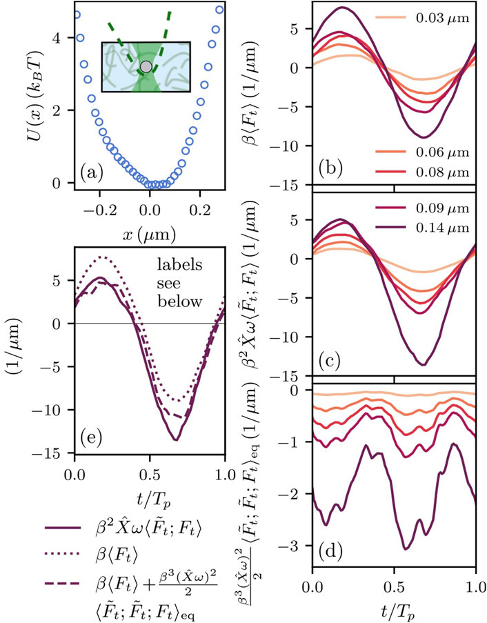
Figure 1. (a) Asymmetric optical potential
To apply the driving protocol, the sample cell is moved, whereas the optical trap remains stationary in our experiments. This is achieved using a piezo-driven stage, on which the sample is mounted and translated in an oscillating manner relative to the trap. In the fluid’s rest frame, this yields a periodic motion of the potential minimum
with the amplitude
Data analysis
With the protocol of Equation 3, Equation 2 takes, expanded to the second order, the form
where the tilde denotes the cosine transform, i.e.,
The cumulants in Equation 4 depend on time
Figure 1c shows the force covariance for the same parameters and color code. For small amplitude
Figure 1d shows the third cumulant of force for the same parameters and color code. We have here restricted to the equilibrium cumulant as it appears in Equation 4, multiplied by
Equation 4 states that in the shown range of amplitudes, the curves in Figure 1c are given by the sum of the curves in Figures 1b,d. For
To test this prediction systematically, we dissect the curves in Figures 1b–d into the contributions from harmonics with frequencies
where the coefficients
Results
Figure 2 shows the coefficients
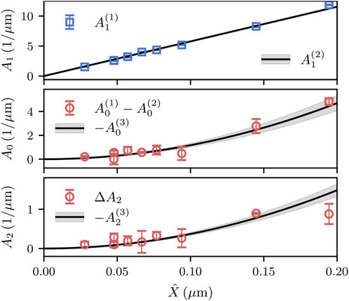
Figure 2. Coefficients
The center and lower panels in Figure 2 show the orders
As data in the top panel of Figure 2 grow linearly and those in the center and lower panels grow quadratically with
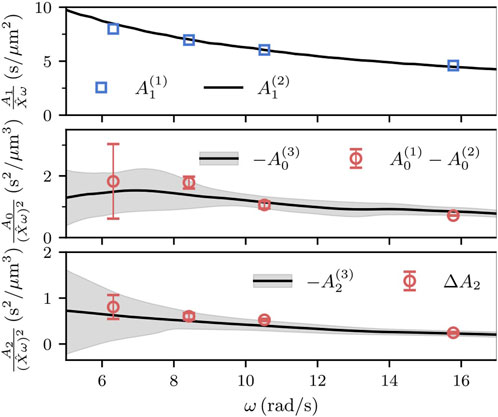
Figure 3. Coefficients
Figure 4 provides the final test of Equation 4, namely, the phases
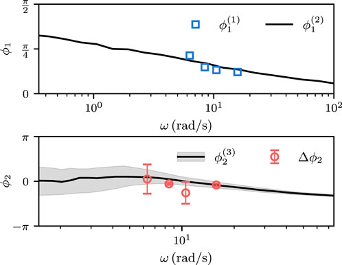
Figure 4. Phase angles
The lower panel shows the phase for
Conclusion
We presented and tested a nonequilibrium fluctuation expansion for a driven classical system, emphasizing the validity on various length scales. Indeed, such relations are necessary, e.g., for a systematic coarse graining of nonequilibrium systems. The identity is confirmed for experiments of a Brownian particle interacting with a complex surrounding. Future work can explore other systems and aim to clarify the relation to the mentioned fluctuation theorems [33, 41]. It is also important to investigate the use of Equation 2 for treating systems far away from equilibrium.
This project was funded by the Deutsche Forschungsgemeinschaft (DFG), Grant No. SFB 1432 (Project ID 425217212)—Project C05.
Data availability statement
The raw data supporting the conclusions of this article will be made available by the authors, without undue reservation.
Author contributions
JC: Writing – review and editing, Writing – original draft. KK: Writing – original draft, Writing – review and editing. CB: Writing – original draft, Writing – review and editing. MK: Writing – review and editing, Writing – original draft.
Funding
The author(s) declare that financial support was received for the research and/or publication of this article. This project was funded by the Deutsche Forschungsgemeinschaft (DFG), Grant No. SFB 1432 (Project ID 425217212)—Project C05. The authors acknowledge support by the Open Access Publication Funds of the Göttingen University.
Conflict of interest
The authors declare that the research was conducted in the absence of any commercial or financial relationships that could be construed as a potential conflict of interest.
Generative AI statement
The author(s) declare that no Generative AI was used in the creation of this manuscript.
Any alternative text (alt text) provided alongside figures in this article has been generated by Frontiers with the support of artificial intelligence and reasonable efforts have been made to ensure accuracy, including review by the authors wherever possible. If you identify any issues, please contact us.
Publisher’s note
All claims expressed in this article are solely those of the authors and do not necessarily represent those of their affiliated organizations, or those of the publisher, the editors and the reviewers. Any product that may be evaluated in this article, or claim that may be made by its manufacturer, is not guaranteed or endorsed by the publisher.
Supplementary material
The Supplementary Material for this article can be found online at: https://www.frontiersin.org/articles/10.3389/fphy.2025.1667224/full#supplementary-material
Footnotes
1The expansion in Equation 2 suggests the dimensionless expansion parameter
2ω is determined from the power spectral density, thus carrying an error depending on the length of the measurement.
3As the phases
References
1. Callen HB, Welton TA. Irreversibility and generalized noise. Phys Rev (1951) 83:34–40. doi:10.1103/physrev.83.34
2. Kubo R. The fluctuation-dissipation theorem. Rep Prog Phys (1966) 29:255–84. doi:10.1088/0034-4885/29/1/306
5. Rytov SM, Kravtsov IA, Tatarskii V. Principles of statistical radiophysics. Springer-Verlag (1987).
6. Hansen JP, McDonald IR. Theory of simple liquids: with applications to soft matter. Elsevier Science (2013).
7. Cugliandolo LF, Dean DS, Kurchan J. Fluctuation-dissipation theorems and entropy production in relaxational systems. Phys Rev Lett (1997) 79:2168–71. doi:10.1103/physrevlett.79.2168
8. Ruelle D. General linear response formula in statistical mechanics, and the fluctuation-dissipation theorem far from equilibrium. Phys Lett A (1998) 245:220–4. doi:10.1016/s0375-9601(98)00419-8
9. Crisanti A, Ritort F. Violation of the fluctuation–dissipation theorem in glassy systems: basic notions and the numerical evidence. J Phys A: Math Gen (2003) 36:R181–290. doi:10.1088/0305-4470/36/21/201
10. Harada T, Sasa S-I. Equality connecting energy dissipation with a violation of the fluctuation-response relation. Phys Rev Lett (2005) 95:130602. doi:10.1103/physrevlett.95.130602
11. Speck T, Seifert U. Restoring a fluctuation-dissipation theorem in a nonequilibrium steady state. EPL (2006) 74:391–6. doi:10.1209/epl/i2005-10549-4
12. Deutsch JM, Narayan O. Energy dissipation and fluctuation response for particles in fluids. Phys Rev E (2006) 74:026112. doi:10.1103/physreve.74.026112
13. Chetrite R, Falkovich G, Gawedzki K. Fluctuation relations in simple examples of non-equilibrium steady states. J Stat Mech (2008):P08005. doi:10.1088/1742-5468/2008/08/P08005
14. Marconi UMB, Puglisi A, Rondoni L, Vulpiani A. Fluctuation–dissipation: response theory in statistical physics. Phys Rep (2008) 461:111–95. doi:10.1016/j.physrep.2008.02.002
15. Saito K. Energy dissipation and fluctuation response in driven quantum langevin dynamics. Europhys Lett (2008) 83:50006. doi:10.1209/0295-5075/83/50006
16. Baiesi M, Maes C, Wynants B. Fluctuations and response of nonequilibrium states. Phys Rev Lett (2009) 103:010602. doi:10.1103/physrevlett.103.010602
17. Prost J, Joanny J-F, Parrondo JMR. Generalized fluctuation-dissipation theorem for steady-state systems. Phys Rev Lett (2009) 103:090601. doi:10.1103/physrevlett.103.090601
18. Harada T. Macroscopic expression connecting the rate of energy dissipation with the violation of the fluctuation response relation. Phys Rev E (2009) 79:030106. doi:10.1103/physreve.79.030106
19. Krüger M, Fuchs M. Fluctuation dissipation relations in stationary states of interacting brownian particles under shear. Phys Rev Lett (2009) 102:135701. doi:10.1103/physrevlett.102.135701
20. Seifert U, Speck T. Fluctuation-dissipation theorem in nonequilibrium steady states. EPL (2010) 89:10007. doi:10.1209/0295-5075/89/10007
21. Baiesi M, Maes C, Wynants B. The modified sutherland–einstein relation for diffusive non-equilibria. Proc R Soc A: Math Phys Eng Sci (2011) 467:2792–809. doi:10.1098/rspa.2011.0046
22. Cugliandolo LF. The effective temperature. J Phys A: Math Theor (2011) 44:483001. doi:10.1088/1751-8113/44/48/483001
23. Verley G, Chétrite R, Lacoste D. Modified fluctuation-dissipation theorem for general non-stationary states and application to the glauber–ising chain. J Stat Mech (2011):10025. doi:10.1088/1742-5468/2011/10/P10025
24. Altaner B, Polettini M, Esposito M. Fluctuation-dissipation relations far from equilibrium. Phys Rev Lett (2016) 117:180601. doi:10.1103/physrevlett.117.180601
25. Lippiello E, Baiesi M, Sarracino A. Nonequilibrium fluctuation-dissipation theorem and heat production. Phys Rev Lett (2014) 112:140602. doi:10.1103/physrevlett.112.140602
26. Wu W, Wang J. Generalized fluctuation-dissipation theorem for non-equilibrium spatially extended systems. Front Phys (2020) 8:567523. doi:10.3389/fphy.2020.567523
27. Caprini L. Generalized fluctuation–dissipation relations holding in non-equilibrium dynamics. J Stat Mech (2021):063202. doi:10.1088/1742-5468/abffd4
28. Baldovin M, Caprini L, Puglisi A, Sarracino A, Vulpiani A. In nonequilibrium thermodynamics and fluctuation kinetics: modern trends and open questions. Springer International Publishing (2022).
29. Johnsrud MK, Golestanian R, Generalized fluctuation dissipation relations for active field theories (2024), arXiv:2409.14977.
30. Kubo R. Statistical-mechanical theory of irreversible processes. I. General theory and simple applications to magnetic and conduction problems. J Phys Soc Jpn (1957) 12:570–86. doi:10.1143/jpsj.12.570
31. Bernard W, Callen HB. Irreversible thermodynamics of nonlinear processes and noise in driven systems. Rev Mod Phys (1959) 31:1017–44. doi:10.1103/revmodphys.31.1017
32. Efremov GF, Eksp Z. A fluctuation dissipation theorem for nonlinear media. Theor Fiz (1968) 55:2322.
33. Bochkov GN, Kuzovlev YE. Nonlinear fluctuation-dissipation relations and stochastic models in nonequilibrium thermodynamics. Phys A: Stat Mech Appl (1981) 106:443–79. doi:10.1016/0378-4371(81)90122-9
34. Stratonovich RL. Nonlinear nonequilibrium thermodynamics I: Linear and nonlinear fluctuation-dissipation theorems. Springer (1992).
35. Evans DJ, Morriss G. Statistical mechanics of nonequilibrium liquids. 2nd ed. Cambridge University Press (2008).
36. Fuchs M, Cates ME. Integration through transients for Brownian particles under steady shear. J Phys Condens Matter (2005) 17:S1681–96. doi:10.1088/0953-8984/17/20/003
37. Holsten T, Krüger M. Thermodynamic nonlinear response relation. Phys Rev E (2021) 103:032116. doi:10.1103/PhysRevE.103.032116
38. Oppenheim I. Nonlinear response and the approach to equilibrium. Prog Theor Phys Supp (1989) 99:369–81. doi:10.1143/ptps.99.369
39. Bouchaud J-P, Biroli G. Nonlinear susceptibility in glassy systems: a probe for cooperative dynamical length scales. Phys Rev B (2005) 72:064204. doi:10.1103/physrevb.72.064204
40. Lippiello E, Corberi F, Sarracino A, Zannetti M. Nonlinear response and fluctuation-dissipation relations. Phys Rev E (2008) 78:041120. doi:10.1103/physreve.78.041120
41. Andrieux D, Gaspard P. Quantum work relations and response theory. Phys Rev Lett (2008) 100:230404. doi:10.1103/physrevlett.100.230404
42. Lucarini V, Colangeli M. Beyond the linear fluctuation-dissipation theorem: the role of causality. J Stat Mech (2012):p05013. doi:10.1088/1742-5468/2012/05/P05013
43. Diezemann G. Nonlinear response theory for markov processes: simple models for glassy relaxation. Phys Rev E (2012) 85:051502. doi:10.1103/physreve.85.051502
44. Wang E, Heinz U. Generalized fluctuation-dissipation theorem for nonlinear response functions. Phys Rev D (2002) 66:025008. doi:10.1103/physrevd.66.025008
45. Andrieux D, Gaspard P. A fluctuation theorem for currents and non-linear response coefficients. J Stat Mech (2007):P02006. doi:10.1088/1742-5468/2007/02/P02006
46. Colangeli M, Maes C, Wynants B. A meaningful expansion around detailed balance. J Phys A: Math Theor (2011) 44:095001. doi:10.1088/1751-8113/44/9/095001
47. Basu U, Krüger M, Lazarescu A, Maes C. Frenetic aspects of second order response. Phys Chem Chem Phys (2015) 17:6653. doi:10.1039/C4CP04977B
48. Basu U, Helden L, Krüger M. Extrapolation to nonequilibrium from coarse-grained response theory. Phys Rev Lett (2018) 120:180604. doi:10.1103/PhysRevLett.120.180604
49. Maes C. Response theory: a trajectory-based approach. Front Phys (2020) 8:229. doi:10.3389/fphy.2020.00229
50. Caspers J, Krüger M. Nonlinear langevin functionals for a driven probe. J Chem Phys (2024) 161:124109. doi:10.1063/5.0227674
51. Helden L, Basu U, Krüger M, Bechinger C. Measurement of second-order response without perturbation. EPL (2016) 116:60003. doi:10.1209/0295-5075/116/60003
52. Maes C. On the second fluctuation–dissipation theorem for nonequilibrium baths. J Stat Phys (2014) 154:705–22. doi:10.1007/s10955-013-0904-8
53. Maes C. Frenesy: time-Symmetric dynamical activity in nonequilibria. Phys Rep (2020) 850:1–33. doi:10.1016/j.physrep.2020.01.002
54. Gomez-Solano JR, Petrosyan A, Ciliberto S, Chetrite R, Gawedzki K. Experimental verification of a modified fluctuation-dissipation relation for a micron-sized particle in a nonequilibrium steady state. Phys Rev Lett (2009) 103:040601. doi:10.1103/physrevlett.103.040601
55. Blickle V, Speck T, Lutz C, Seifert U, Bechinger C. Einstein relation generalized to nonequilibrium. Phys Rev Lett (2007) 98:210601. doi:10.1103/physrevlett.98.210601
56. Mehl J, Blickle V, Seifert U, Bechinger C. Experimental accessibility of generalized fluctuation-dissipation relations for nonequilibrium steady states. Phys Rev E (2010) 82:032401. doi:10.1103/physreve.82.032401
57. Gomez-Solano JR, Petrosyan A, Ciliberto S, Maes C. Fluctuations and response in a non-equilibrium micron-sized system. J Stat Mech (2011):P01008. doi:10.1088/1742-5468/2011/01/P01008
58. Bochkov GN, Kuzovlev YE. General theory of thermal fluctuations in nonlinear systems. Zh Eksp Teor Fiz (1977) 72:238.
59. Jarzynski C. Nonequilibrium equality for free energy differences. Phys Rev Lett (1997) 78:2690–3. doi:10.1103/physrevlett.78.2690
60. Crooks GE. Entropy production fluctuation theorem and the nonequilibrium work relation for free energy differences. Phys Rev E (1999) 60:2721–6. doi:10.1103/physreve.60.2721
61. Seifert U. Stochastic thermodynamics, fluctuation theorems and molecular machines. Rep Prog Phys (2012) 75:126001. doi:10.1088/0034-4885/75/12/126001
62. Caspers J, Krüger M. Identities for nonlinear memory kernels. Phys Rev E (2025) 112:024124. doi:10.1103/pzs6-l3ws
63. Maes C. Local detailed balance. Scipost Phys Lect Notes (2021) 32. doi:10.21468/scipostphyslectnotes.32
64. Cates ME, Candau SJ. Statics and dynamics of worm-like surfactant micelles. J Phys Condens Matter (1990) 2:6869–92. doi:10.1088/0953-8984/2/33/001
Keywords: fluctuation–dissipation theorem, nonequilibrium cumulants, Brownian probe particle, optical potential, nonlinear fluid, non-Markovian fluid, worm-like micelles, micellar fluid
Citation: Caspers J, Krishna Kumar K, Bechinger C and Krüger M (2025) Equilibrium trajectories quantify second-order violations of the fluctuation–dissipation theorem without the need for a model. Front. Phys. 13:1667224. doi: 10.3389/fphy.2025.1667224
Received: 16 July 2025; Accepted: 18 September 2025;
Published: 21 October 2025.
Edited by:
Andre P. Vieira, University of São Paulo, BrazilReviewed by:
Saravana Prakash Thirumuruganandham, SIT Health, EcuadorPedro Harunari, University of Luxembourg, Luxembourg
Copyright © 2025 Caspers, Krishna Kumar, Bechinger and Krüger. This is an open-access article distributed under the terms of the Creative Commons Attribution License (CC BY). The use, distribution or reproduction in other forums is permitted, provided the original author(s) and the copyright owner(s) are credited and that the original publication in this journal is cited, in accordance with accepted academic practice. No use, distribution or reproduction is permitted which does not comply with these terms.
*Correspondence: Juliana Caspers, ai5jYXNwZXJzQHRoZW9yaWUucGh5c2lrLnVuaS1nb2V0dGluZ2VuLmRl; Matthias Krüger, bWF0dGhpYXMua3J1Z2VyQHVuaS1nb2V0dGluZ2VuLmRl