Computation of Thickness and Mechanical Properties of Interconnected Structures: Accuracy, Deviations, and Approaches for Correction

Introduction

Lacking a detailed morphological and topological description of the microstructure, the structure-property relationship of open-pore materials, such as metal foams, elastomeric foams, or Nanoporous gold (NPG) is commonly described by the Gibson-Ashby scaling law, in which the solid fraction is the most important parameter characterizing the materials morphology (Gibson and Ashby, 1997; Ashby et al., 2000). During the last two decades, the morphological characterization and prediction of mechanical properties of open-pore materials gained increasing attention, thanks to the improving resolution of X-ray, FIB, and TEM micro-/nanotomography instruments, complemented by advancing image processing algorithms and computational modeling techniques. Tomography and FEM simulations on metal and elastomeric foams date back to Nieh et al. (1998), Nieh et al. (2000), and Kinney et al. (2001). A very detailed analysis of cell volume and strut length distributions, number of faces per cell, junctions coordination number and the shape of the most representative cells was carried out by Dillard et al. (2005) based on a 3D quantitative image analysis of open-cell nickel foams under tension and compression loading using X-ray microtomography.

First studies based on NPG were conducted by Rösner et al. (2007) using TEM on dealloyed gold leafs. Hu et al. (2016), Mangipudi et al. (2016), and (Ziehmer et al., 2016) analyzed NPG samples of larger volumes, obtained from focused ion beam (FIB) sectioning and scanning electron microscope (SEM) imaging. By these thorough works, a systematic analysis of the NPG morphology in terms of ligament size distribution and connectivity density has become possible for the first time. Because the ligaments are of nanoscale dimension, these investigations are all based on high-resolution SEM images for which techniques for an automated image processing are an asset. Hu et al. (2016) and Mangipudi et al. (2016) use the 3D Biggest Sphere Thickness algorithm by Hildebrand and Rüegsegger (1997) for the estimating the ligament size distribution of 3D volumes.

For the geometrical description of the ligaments in a NPG network, Pia and Delogu (2015) proposed a parabolic shape with a square cross-section connected in cubic nodes. The parameters for the parabolic shape and their statistical distribution were manually determined from 2D SEM images. Badwe et al. (2017) analyzed 2D SEM images using digital image analysis to obtain ligament size histograms that were fit to the Weibull distribution. To obtain the ligament size distribution, they apply the skeletonization and distance map transformation each onto the original binary SEM image, using the open-source software ImageJ. The multiplication of these two results yields the skeleton ascribed with the according diameter at each skeleton-point. Consistent with the results of Rösner et al. (2007) and Hu et al. (2016), the mean ligament distributions were reported to be nearly self-similar for the examined ligament sizes. Stuckner et al. (2017) present a Python package AQUAMI, which automatically analyzes microstructural features from micrographs. The approach is similar to the approach by Badwe et al. (2017), which was independently published, but has no need for manual calculation in ImageJ. The average diameter and diameter distribution of the morphologies in each phase is calculated using a medial axis transform and a distance transform. McCue et al. (2018) use AQUAMI to data-mine NPG 2D images of 28 published manuscripts, regarding mean ligament diameter, length, and solid phase fraction. They point out the difficulty and resulting systematic discrepancies when comparing results gained by different measuring approaches, ranging from manually measuring the thinnest part of the ligament, to computational estimations. Furthermore, as a minimum criterion for meaningful image analysis, they propose to use images with a minimum resolution of at least 10 pixels per ligament diameter, due to the otherwise reported errors.

In summary, two algorithms are found to be dominantly used in literature to estimate the ligament size distribution: The Thickness algorithm, which is able to analyze 3D volumes and the Euclidean distance transformation (EDT), which is applied for analyzing 2D SEM images by Badwe et al. (2017), Stuckner et al. (2017), and McCue et al. (2018). It calculates at each point of the structure the distance to the nearest background point. The Thickness algorithm by Hildebrand and Rüegsegger (1997) is implemented in image analysis programs, such as the open-software program Fiji by Schindelin et al. (2012). It calculates the local thickness at a point as the dimeter of the largest sphere, which is completely inside the structure and which contains the evaluated point. The mean thickness is calculated as the volume weighted average of the local thickness. The algorithm is commonly used to estimate the mean trabecular thickness of trabecular bone (Day et al., 2000; Almhdie-Imjabber et al., 2014), or other bone structures (Witkowska et al., 2014), because it is a powerful and fast volume-based algorithm. In the context of NPG the Thickness algorithm has been applied for analyzing 3D tomography data or voxel models by Hu et al. (2016), Mangipudi et al. (2016), Richert and Huber (2018), and Soyarslan et al. (2018a,b).

By the definition of Hildebrand and Rüegsegger (1997), the biggest sphere at a skeleton point p_skel does not need to be centered at this point. Liu et al. (2014) show for an object formed by two overlapping disks of different scales that the Thickness algorithm shows a bias toward the larger disk. They furthermore show that an equivalently working Smallest Sphere approach results in the same artifact, but in the opposite direction. The authors propose the definition of the thickness of a point p as the diameter of the maximum inscribed sphere whose circumference is farthest from p. Furthermore, for the skeleton, the property must be satisfied that the thickness at a skeleton point p_skel is the diameter of the biggest sphere centered at p_skel. They introduced also a star-line-based algorithm, where the thickness at an axial voxel is defined as the minimum-intercept of a straight line with the boundary. The minimum-intercept length measure is highly robust under small random shifts of axial voxels. One drawback of this thickness computation method lies in the increased computation time needed, because interpolated intensity values at multiple sample points have to be computed on individual star-lines for each axial voxel. For more details and other thickness approaches see also the literature cited by Liu et al. (2014). The tendency to overpredict the thickness of structures was also reported by Maier et al. (2017) for cartilage thickness, in comparison to other thickness estimation approaches. Such an overprediction is unproblematic when studying the self-similarity of structures, or when comparing mean values or distributions. However, for the prediction of mechanical properties using FEM, the correct diameter distribution along the ligament axis is crucial. Richert and Huber (2018) showed that the Thickness algorithm reaches its limits when being applied to typical shapes of NPG ligaments, due to the strongly varying diameter along the ligament axis. The resulting overestimation in ligament radius up to 30% has a strong impact on the predicted mechanical stiffness, which can deviate by a factor of more than two. In their conclusions, Richert and Huber (2018) mentioned the need for a correction method for tracing back an identified ligament shape to the corresponding true geometry, which could be based on inverse methods, such as optimization or machine learning. This important finding has been ignored by Soyarslan et al. (2018b) who used the diameter information as determined from the Thickness algorithm in their beam-FE model, without any local validation of the detected diameters or discussion of possible consequences for their mechanical prediction.

Further literature research revealed that there exists also a plugin in the open-software program Fiji of the 3D Euclidean distance transformation (EDT) by Ollion et al. (2013), among others, which seems to be unnoticed by groups working on the analysis of 3D data. As this algorithm computes the distance from a given voxel of the structure to the nearest background voxel, the extracted axis-to-surface distance will have the tendency to underpredict the ligament diameter for highly convex or concave ligament shapes. The reason for this is that the smallest distance is determined by the normal from the surface contour to an axis point, which is smaller compared to the diameter measured normal to the ligament axis. It his however unclear, how large the deviations are for the typical geometries found in open pore materials and how big their impact is on the mechanical properties in comparison to the results from the Thickness algorithm.

Motivated by these findings, this paper aims to lay a solid basis for error estimation and thickness correction for the different algorithms. The availability of a method for an accurate characterization represents a key element for producing data sets of high quality, consisting of pairs of structure information and related mechanical properties. As demonstrated by Huber (2018) for the topology term of the structure-property relationship, a larger number of such patterns is needed for deriving a fairly general representation using data mining and machine learning approaches. This is particularly an issue when pooling data from different sources, which make use of different algorithms.

Following a detailed investigation of the sources of over- and underestimation in the computed thickness data, approaches for the correction of data from the Thickness algorithm are proposed: A Smallest Ellipse algorithm, which resides in between the Biggest Sphere approach and the Smallest Sphere approach, and an artificial neural network approach. Similarly, an artificial neural network approach is proposed for the correction of data from the Euclidean distance transformation. The results clearly show that the artificial neural network is able to correct the over- and underpredicted thickness dependent on the position of the ligament axis. The drawback is that it is limited to the range of ligament shapes used during training. Recommendations are given in terms of generalization to asymmetric ligaments as a requirement for applications to larger structures of higher complexity.

Methodology

Previous analysis by Richert and Huber (2018) on actual NPG tomography data produced by Hu et al. (2016) revealed a diameter overestimation of the NPG structure by the Biggest Sphere Thickness algorithm by Hildebrand and Rüegsegger (1997), implemented in the open-source program Fiji by Schindelin et al. (2012), in the Thickness Plugin by Dougherty and Kunzelmann (2007). Richert and Huber (2018) mathematically calculated the influence on the overestimated ligament diameters on the mechanical stiffness for single parabolic ligaments, showing an overestimation by up to a factor of 8. These results clearly show the significance of the error to be expected as function of the ligament geometry, but it is unclear how strong this effect is reflected in the macroscopic properties of a Representative Volume Element (RVE). It can be argued that the macroscopic response of an interconnected structure could be less sensitive to local deviations in the ligament geometries. Furthermore, the amount and effect of possible underestimations by the distance transformation need to be investigated. An impression of the discrepancy between the two algorithms is obtained by analyzing the tomography data of Hu et al. (2016), shown in Figure 1. The Thickness (Th) and Euclidean distance transformation (EDT) information are consistently evaluated along the skeleton voxels. It can be seen that the determined averages of 400 nm (Th) and 308 nm (EDT) deviate significantly. It is therefore important to investigate each algorithm with respect to ligament shape and to propose correction methods, where needed.

FIGURE 1

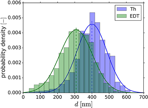
Figure 1. Ligament diameter distribution of NPG tomography with Thickness (Th) and Euclidean distance transformation (EDT) algorithm. The histograms are normalized to an area of one and fitted with the Gaussian distribution. Shifted distributions with average ligament diameter of 400 nm (Th) and 308 nm (EDT) are observed.

It should be noted that working with tomography data, several crucial image-processing steps are necessary beforehand, such as image noise filtering, brightness and contrast adjustment, registration and segmentation. For the latter, it is necessary to set a threshold value that decides if a voxel is attributed to the solid or to the pore space and the proper choice of this parameter is absolutely critical for all following steps. Commonly, this parameter is calibrated via the relative density of the material, which is independently measured. While this ensures that the tomography reflects the relative density of the material in average, this does not guarantee that local features are precisely detected. In case of the NPG-epoxy composite tomography data produced by Hu et al. (2016), specific settings in the FIB-SEM process made the ligaments easily distinguishable without interfering with the ligament network structure underneath the cross-section. In this case, the segmentation in Fiji using a single value gray-scale threshold for the image stack was thus applicable. An image processing error of ±2% in volume fraction was found by manually changing the image contrast, brightness and threshold value for the segmentation process for that data set (Hu, 2017).

This study focuses on analyzing the influence of the Thickness and EDT algorithm on NPG-like RVEs, which are based on known geometries. Emphasis is placed on providing data of sufficiently complex but well-defined 3D structures, for which the exact diameter information is known in each position along the ligament axis. To this end, ligaments with a smooth parabolic-spherical ligament shape as suggested by Richert and Huber (2018) are organized in a diamond structure. This topology is frequently used for mechanical modeling of 3D open pore materials (Nachtrab et al., 2011; Huber et al., 2014; Roschning and Huber, 2016; Jiao and Huber, 2017a,b; Huber, 2018). In contrast to the conventional FEM approaches, which are computational expensive, FEM beam models allow for fast computation even for large plastic deformation, which is a requirement for larger parameter studies of larger and more realistic RVEs. The drawback of this method is the underprediction of stiffness and strength, which needs to be compensated via a correction of the nodal mass (Huber et al., 2014; Roschning and Huber, 2016; Jiao and Huber, 2017b). An attractive alternative for the numerical simulation of foam-like materials is the Finite Cell Method (Parvizian et al., 2007; Düster et al., 2008, 2017). Recently, Gnegel et al. (2019) applied this approach for predicting the elastic-plastic deformation behavior of pure and polymer coated NPG based on the tomography data of Hu et al. (2016). In combination with experimental macroscopic compression data, it was possible to determine the elastic-plastic properties of the gold phase and of the polypyrrole coating of a few nanometer thickness. This requires reducing the explicitly modeled 3D structure to a sub-sample of the available tomography dataset such that the model could be computed in a reasonable time. Therefore, FEM beam models remain an attractive candidate for computing larger models.

For the sake of a systematic in-depth comparison of all methods under investigation, the geometries in this work are limited to symmetric shapes. Altogether, 16 idealized model geometries plus three additional validation geometries are generated covering the relevant range of ligament shapes from concave to convex. For each model geometry, a high-resolution voxel representation serves as basis for testing various approaches of thickness detection and correction. In addition to the assessment of the error in the determined geometry, the effect on the mechanical properties is computed for each structure and correction method using the FEM beam modeling approach developed in a series of previous works (Huber et al., 2014; Jiao and Huber, 2017a; Huber, 2018; Richert and Huber, 2018).

Motivated by the reported differences between the skeleton FEM beam model and the FEM solid model (Richert and Huber, 2018), FEM solid models are created via PCL scripting in MSC Patran, complementing the reference FEM beam models. The results will provide further insights into the differences between FEM beam and FEM solid models for various ligament shapes in terms of elastic and plastic deformation behavior. The results are also relevant for the further development of nodal corrections for more general ligament shapes as an extension to the simple ball-and-stick geometries investigated by Jiao and Huber (2017b).

Figure 2 gives an overview of the workflow applied in the following sections. Details on the individual approaches are provided at the beginning of each section. To mimic the FEM skeleton beam model building process from tomography data by Richert and Huber (2018), the RVE geometry information is scanned by a Python script with a defined voxel resolution. The output is a voxelized tiff stack, which is needed as input for the Skeletonize, AnalyzeSkeleton, Thickness and 3D Distance Map Plugin evaluations in Fiji (Lee et al., 1994; Dougherty and Kunzelmann, 2007; Arganda-Carreras et al., 2010; Ollion et al., 2013). The whole procedure of building the FEM skeleton beam model from tomography data is described in detail in the Appendix of Richert and Huber (2018). The simulation of the original FEM beam model vs. the FEM skeleton beam model created with the Thickness information will reveal the impact of the flawed diameter estimation on the mechanical behavior of the ligament network. This allows us also to individually analyze the errors originating from the voxel resolution, the skeletonization, and the ligament discretization on the macroscopic elastic-plastic response.

FIGURE 2

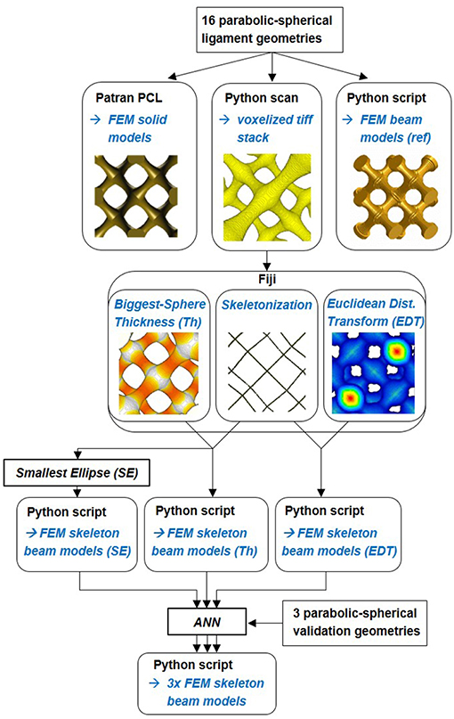
Figure 2. Workflow of the geometry computation and FEM model creation. 1st step: Reference FEM solid model, voxelized image stack, and reference FEM beam model are built. 2nd step: Skeletonization, Thickness estimation, and Euclidean distance transformation are done in Fiji. 3rd step: FEM skeleton beam models are built via python scripting with Thickness (Th), Euclidean distance transformation (EDT), and corrected diameters using the Smallest Ellipse (SE). 4th step: additional artificial neural network (ANN) correction approach.

After the analysis of the influencing parameters with regard to their effect on the geometry computation, the question arises, to what extend the error of each algorithm could be reduced in the aftermath. Concerning the Thickness algorithm we focus in this work on two different correction approaches. Geometrically it is clear why the Thickness algorithm overestimates the diameters of strongly varying ligament shapes as found in NPG. This is why a direct reconstruction approach is developed, opting for an ellipse as the final scanning volume. This so-called Smallest Ellipse (SE) algorithm resides in between the Biggest Sphere approach and the Smallest Sphere approach and is therefore a promising technique for efficiently balancing the thickness data between over and underprediction. A second correction approach is based on an artificial neural network (ANN), which efficiently allows for a global mapping from the measured overpredicted to the corrected ligament shapes. The ANN approach is also applied for correcting data from the EDT algorithm.

Reference FEM Models and Their Properties

Reference Geometry of the Unit Cell

To study the effect of the overestimation in the thickness and the quality of approaches for correction, 16 diamond unit cells are generated. By shifting the diamond structure proposed by Huber et al. (2014) by a quarter of a unit cell length in all three coordinate directions (Soyarslan et al., 2017), four ligaments with complete nodes at both ends are positioned in the center of the RVE. These core ligaments are later analyzed with respect to their thickness distribution by different algorithms, as they remain unaffected by cuts at the boundary of the RVE.

In what follows, the investigation of the mechanical behavior is limited to macroscopic compression, which is commonly used in experiments (Jin et al., 2009; Huber et al., 2014; Hu et al., 2016; Liu and Jin, 2017). The resulting macroscopic properties are only valid for this loading direction. Due to the inherent anisotropy in the diamond structure, the mechanical response can be different for compression, tension, and shear. The elastic properties though can be considered isotropic in tension and compression, because elastic properties per definition reflect small deformations. Furthermore, because of the perfect symmetry of the unit cell in x, y, and z-direction, isotropy in these directions is naturally given as long as the loading is consistently either tension or compression. Thus, the stress-strain curve will show perfect agreement for small strains, whereas with increasing strain, the stress-strain curves for tensile loading tends to rise faster compared to the curves for compression loading. Under tensile loading, the ligaments tend to align in loading direction (see Sun et al., 2013) and are able to bear higher loads compared to compression loading, where the ligaments deform like an s-shape due to bending (Huber et al., 2014). Therefore, the yield strength is slightly larger in tension than in compression and the difference is more pronounced for thin ligaments, because they align more easily in tensile direction like fibers. These mechanisms are demonstrated for two example structures G₁₁ and G₁₄ in Supplementary Section 2.3. For the scope of this work it is sufficient to concentrate on compression, because errors in the ligament geometry will be reflected similarly in all mechanical properties and loading scenarios. In what follows, we will investigate the errors in the thickness determination depending on the algorithm that is used and their correction. To this end, we use diamond structure consisting of identical ligaments with well-known geometry. Because of this replication, the macroscopic behavior of the structure gives an indication about the response of a single ligament that is part of a more complex network.

Variable ligament shapes are incorporated in form of a continuous parabolic-spherical shape introduced by Richert and Huber (2018), see Figure 10 therein. To incorporate also asymmetric ligament shapes observed by Richert and Huber (2018), the ends are defined by two different radii r_{end, l} and r_{end, r} for the left and right junction, respectively. The resulting gradient along the ligament with length l is included in Equation (1) through the parameter b. The locations x_{Q, l} and x_{Q, r} at which the parabolic shape transitions into the spherical parts of the ligament, are determined iteratively such that a smooth ligament with a tangential transition is achieved (see Richert and Huber, 2018).

$\begin{array}{ll}r\left(x\right)=\{\begin{array}{ll}\sqrt{r_{end,l}^2-{(l/2+x)}^2}\hfill & -l/2\le x<x_{Q,l}\hfill \\ a{x}^2+bx+c\hfill & x_{Q,l}\le x\le x_{Q,r}\hfill \\ \sqrt{r_{end,r}^2-{(l/2-x)}^2}\hfill & x_{Q,r}<x\le l/2\hfill \end{array}& (1)\end{array}$

The axial coordinate x has its origin in the mid of the ligament, such that the ligament mid radius is given by r_mid = c. For the in-depth study of the thickness determination and correction as well as their effect on the mechanical properties, the ligament shape is kept symmetric by setting b = 0. In this case, r_end = r_{end, l} = r_{end, r} and x_{Q, l} = − x_{Q, r}.

In what follows, the unit cell size a_UC is set to 1, i.e., all absolute lengths are given as fraction of the unit cell size. The 16 geometries are chosen to cover ratios of ligament mid to end radius r_mid/r_end from 0.5 to 1.25 in increments of 0.25. This is the relevant range of ligament shapes as identified from a 3D tomography of a NPG sample (Richert and Huber, 2018). As the second geometry parameter, the end radius was varied from r_end = 0.1 to 0.175 in increments of 0.025. Through the combination of these two parameters a large range of solid fractions is covered that exceeds the typical range of NPG samples from very low (φ_min ≈ 0.1) to very large values (φ_max ≈ 0.5). Based on the two chosen parameters r_mid and r_end, the parameter c in Equation (1) can be determined following Richert and Huber (2018).

Reference FEM Solid and Beam Models

Reference FEM beam and solid models are generated for all geometries defined in Table 1. A detailed description of how the reference FEM beam is created is given in Supplementary Section 1. The solid unit cells are built using PCL scripting in MSC Patran 2017 and, after Boolean operation on all ligament and junction volumes, are meshed in a single meshing operation with C3D10 three dimensional 10-node quadratic tetrahedron elements for (Abaqus, 2014). The number of elements range from 9,445 to 38,279 for structures with lowest (G₁₁) and highest solid fraction (G₄₄), respectively, with average element sizes of 0.05. The solid fractions given in Table 1 are obtained from the FEM solid model in Abaqus via the history output VOL. Examples for the most filigree structures with r_end = 0.1 are shown in Figure 3. Due to the small ligament diameter, these structures will show the highest sensitivity with respect to effects of voxel resolution, discretization, and the accuracy of the algorithms applied to these data.

TABLE 1

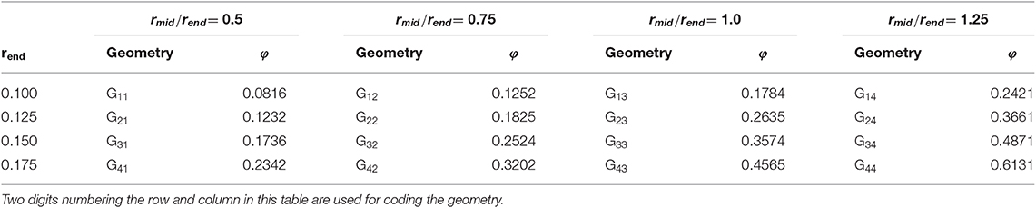
Table 1. Geometry parameters r_mid and r_end, describing the ligament shape, coding of the shapes from possible combinations and resulting solid fractions φ.

FIGURE 3

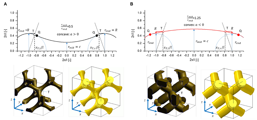
Figure 3. Plots of Equation (1) together with images of unit cells generated for the most filigree structures with r_end= 0.1: (A) Geometry G₁₁, r_mid/r_end= 0.5; (B) Geometry G₁₄, r_mid/r_end= 1.25.

In addition to the solid models that serve as common reference for all mechanical properties, FEM beam models with 20 beam elements per ligament of type B31 [two-node shear flexible Timoshenko beams in space; (Abaqus, 2014)] are built using the code developed by Huber (2018). The code is modified for assigning a variable ligament shape to the beam elements in dependence of their position relative to the mid of the ligaments.

For the mechanical properties, a Young's modulus of E_s = 80 GPa, a Poisson's ratio of ν = 0.42, a yield strength of σ_{y, s} = 500 MPa, and a work-hardening rate of E_T = 1,000 MPa are chosen. These parameters represent the mechanical behavior of the ligaments in NPG reasonably well (Huber et al., 2014; Hu et al., 2016; Roschning and Huber, 2016; Huber, 2018).

The translation of the ligament shape given in Equation (1) for a single ligament into a physical meaningful radius distribution for the interconnected structure is described in detail in Supplementary Section 2. Through the intersection of three convex ligaments, the actual size of the nodal mass increases to the value R, which is defined by the triple point—the point where the surfaces of three ligaments intersect. This surface point is closest to the center of the nodal mass. Therefore, all reference FEM beam models are based on the radius for the biggest sphere R, that fits in the nodal area. The corresponding radii are computed as distance from the center of the junction to the surface in direction of the triple point, which is found at an angle of 70.53° relative to the ligament axis. The value R is assigned to all elements positioned between the ligament end, which is the center of the nodal mass, to the axial position of the triple point T. This approach avoids case sensitivity and allows to compare the results from different models. All geometric parameters for the structures defined in Table 1 are provided in Supplementary Section 4, Supplementary Table 1. Supplementary Figure 6A shows that there is only a moderate effect in the macroscopic Young's modulus. For most ligaments, the stiffening is below 10%. However, for the yield strength shown in Supplementary Figure 6B, the incorporation of R becomes relevant for cylindrical and convex shaped ligaments, for which a strength increase by up to 20% and 40%, respectively, is achieved.

Boundary Conditions

For a finite model size, the choice of the boundary conditions can significantly influence the material response significantly. Miehe and Koch (2002) showed for shearing of a composite microstructure modeled with 2D solid elements that prescribed displacement boundary conditions lead to a stiffer response compared to periodic boundary conditions. Diebels and Steeb (2002) showed that boundary layers of rotations form under simple shear of a foam leading to a size effect. In this study, we investigate the effect of errors in ligament geometry on macroscopic properties and effects of boundary conditions should be avoided. Therefore, the chosen boundary conditions emulate an infinite periodic microstructure. Due to the perfect symmetry of the diamond structure, all simulations can be based on one unit cell with prescribed displacement and rotation boundary conditions, for details see Supplementary Section 1.2. For the FEM beam model, this approach is equivalent to periodic boundary conditions, while it significantly simplifies the meshing of a 3D FEM solid model.

The displacement boundary conditions impose the known deformation behavior of the structure on all surface nodes using ^*EQUATION in Abaqus. To this end, nodes on planes x = 0, y = 0, and z = 0 are set to zero displacement normal to the corresponding plane. Nodes in the planes at coordinate x = 1, y = 1, and z = 1 are set to remain in a plane that is controlled by a dummy node. All nodes on the mid planes are forced to move half the displacement of the corresponding nodes in the plane at coordinate 1. Finally, in the beam models, all rotational degrees of freedom are set to zero for all surface nodes. As no displacement boundary conditions are applied to the five internal junction nodes within the RVE, these nodes are allowed to move and rotate without any constraint. Nevertheless, they behave identically to the nodes at the boundaries, which have their rotational degrees of freedom fixed, and accomplish a full periodicity of the stress and deformation field results. This indicated the correctness of the chosen boundary conditions being equivalent to periodic boundary conditions. More details are given in Supplementary Section 1.2 (see Supplementary Figures 2, 3).

For elastic computations, a compression strain of 1% is applied on the dummy node of plane z = 1; for predicting elastic-plastic stress-strain behavior, the structure is compressed by 20% strain using large deformation theory (NLGEOM) with a start increment of 0.001. The Young's modulus is always determined from the first loading increment.

For geometries G₁₁ and G₁₄ (r_end = 0.1, r_mid/r_end = 0.5 and r_mid/r_end = 1.25, respectively), a size study with RVEs of increasing model size confirmed that the chosen displacement boundary conditions yield results identical to periodic boundary conditions, both being independent of the model size. The results are presented in Supplementary Section 1.2. As shown in Supplementary Figure 3, the computations with simple symmetry conditions, as used e.g., by Huber et al. (2014), asymptotically approach this value with increasing model size (see also the size study in the Appendix of Huber, 2018). For applying the displacement boundary conditions in the solid model, a search tolerance of 1% of the unit cell allows collecting enough FE nodes, which are sufficiently close to the position of the corresponding surface nodes of the FEM beam model.

Figure 4 shows contour plots for the corresponding FEM solid and beam models at a deformation in the elastic-plastic transition. Elements exceeding the yield stress of 500 MPa are colored in gray. They represent the distribution of the plastic zones, which are in good agreement for the solid model and the corresponding beam model for the convex ligament shape G₁₄, as can be seen from Figures 4C,D. However, for structure G₁₁ with concave ligaments shown in Figure 4A, the plastic zones are organized in the FEM solid model along the tension and compression side in the thin regions of the ligaments and cross the junction volume in the middle into the neighboring ligament. Due to the kinematics implemented in the FE beam elements, the FEM beam model in Figure 4B cannot capture this complex deformation and localizes the plastic strains in elements in the transition region from the ligament to the nodal mass.

FIGURE 4

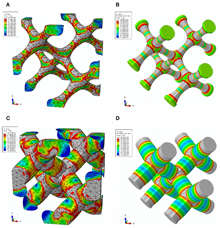
Figure 4. Localization of plastic yield (elements in gray color) during loading after entering the plastic regime for (A) solid model of structure G₁₁; (B) beam model structure G₁₁; (C) solid model of structure G₁₄; (D) beam model of structure G₁₄.

Reference Macroscopic Mechanical Properties

In the following section, the results obtained from the FEM beam model and the FEM solid model are presented for the reference geometries defined in Table 1. This serves two goals. The first goal is to precisely determine the differences between the macroscopic properties of the FEM beam model relative to the FEM solid model of the very same geometry for all ligament geometries. For all further investigations, the FEM beam models serve as reference for the FEM skeleton beam models derived from the voxel models. This allows to clearly separate potential effects from different sources, such as the different behavior of FEM beam and solid models, the thickness algorithms (section FEM Skeleton Beam Models), and the quality assessment of the developed correction methods (section Methods for Thickness Correction).

The macroscopic properties Young's modulus E and the yield strength σ_y are derived from engineering stress and strain measures (see Supplementary Section 1.2, subsection Macroscopic Evaluation). Complete sets of the resulting mechanical properties for the structures defined in Table 1 are provided in form of absolute values in Supplementary Section 4, Supplementary Tables 2–4. An overview of the macroscopic mechanical properties predicted by the reference FEM beam model ($E^{(ref)},{\sigma }_y^{(ref)}$) normalized to the corresponding values of the reference FEM solid model (E, σ_y) is given in Figure 5. The shaded regions indicate solid fractions that are out of the range of NPG (Liu and Jin, 2017; Soyarslan et al., 2018a). It should be noted that a direct comparison with NPG samples via the solid fraction is not possible, because a significant percentage of solid fraction can exist in form of dangling ligaments, whereas our diamond structure is fully connected. Therefore, the larger range of solid fractions in this theoretical work can be useful for covering the relevant ligament shapes determined by Richert and Huber (2018).

FIGURE 5

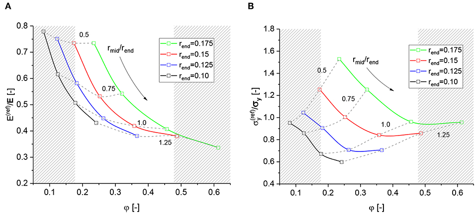
Figure 5. Overview for predicted macroscopic properties from reference FEM beam models normalized to the results from the referenced FEM solid models: (A) Macroscopic Young's modulus; (B) Macroscopic yield strength at 1% plastic strain.

Figure 5A confirms that the FEM beam model generally underpredicts the macroscopic Young's modulus relative to the solid model, which is due to the well-known effect from increased lever length (Huber et al., 2014; Roschning and Huber, 2016). The FEM beam model is more compliant compared to the solid model, because the full distance from the mid of the element to the ligament end, i.e., the half ligament length l/2, is available for bending deformation, independent of the ligament thickness. In contrast to this, the nodal mass in the solid model reduces the lever length available for bending of the ligament depending on the size of the nodal mass relative to the ligament radius. The node is stiffened-up and deformation is moved into the transition zone from the ligament to the nodal mass. For more details, we refer to Huber et al. (2014) and Roschning and Huber (2016). Jiao and Huber (2017b) carried out a study on the effect of the nodal mass for a ball-and-stick model and suggested a nodal corrected beam model to compensate for the softening in the beam model by adjusting the radii and the Young's modulus of the elements in the nodal region.

There is a clear trend toward the stiffness of the solid model for decreasing ratio r_mid/r_end, which goes along with a decreasing solid fraction. This means that the more concave the ligament is, the closer the macroscopic mechanical stiffness is to that of the FEM solid model. Therefore, concave ligaments require less nodal correction to raise the stiffness by about 30% (r_mid/r_end = 0.5) or 80% (r_mid/r_end = 0.75), while cylindrical and convex ligaments require an additional stiffening by more than a factor of 2. This disproves an application of a single “stiffness intensity factor” as proposed by Soyarslan et al. (2018b) independent of the local ligament shape and solid fraction φ.

In contrast to the elastic behavior, the effect in the macroscopic strength, computed at 1% plastic strain, depends strongly on the specific ligament shape (see Figure 5B). In average, the yield strength predicted by the FEM beam model is comparable to that of the FEM solid model. However, for specific ligament shapes the ratio of the yield strength ranges from 0.6 to 1.6. An example is shown in Figures 4A,B. From the contour plots for both types of models it can be deduced that for concave ligament shapes, the plastic zone in the FEM solid model, Figure 4A, is distributed over a larger volume extending from one ligament via the nodal mass into the neighbor ligament. In contrast to this, for the FEM beam model shown in Figure 4B, the plastic deformation localizes in elements located in the transition zone from the ligament to the nodal mass. Therefore, the levers and resulting bending moments causing plastic deformation are longer in the solid model, effectively reducing its mechanical strength. This can explain the unexpected high strength of the FEM beam model for specific geometries.

Based on the good agreement of the yield strength averaged over all geometries, one could argue that a structure that contains a large range of ligament shapes does not require a nodal correction for the mechanical strength. This surprising result has important consequences for the interpretation of stress-strain curves predicted from FEM beam models derived from skeletonized structural data, because the elastic and plastic properties need to be treated differently.

FEM Skeleton Beam Models

The FEM skeleton beam model building approach of Richert and Huber (2018) is based on tomography data sets of real NPG provided by Hu et al. (2016). The common problem for this and similar works (Mangipudi et al., 2016; Soyarslan et al., 2018b) is that the desired thickness information normal to the ligament axis is not easily available. The 16 model geometries, defined in section Reference Geometry of the Unit Cell, enable us to systematically study the different sources of over- and underprediction and to qualify proposed correction methods. Furthermore, the sensitivity with respect to the voxel resolution, the skeletonization, and the discretization of the ligaments is studied.

RVE Size and Voxelization

To mimic the procedure according to the analysis of tomography data, a Python script is used to scan the reference RVEs for given ligament geometries. This scan produces a black (pore) and white (gold) tiff-stack in the chosen voxel resolution. Details on the tomography of the FEM beam models via parallel processing are provided in Supplementary Section 3. The tiff files of the 16 model geometries are available for download as the Data Sheet 2.zip folder of the Supplementary Material. Details of the files are provided in Supplementary Section 5. The code is validated using the open visualization tool Ovito by Stukowski (2010) confirming that the solid fraction of the voxelized model is below 1% error. To avoid boundary issues during the skeletonization and thickness analysis, as discussed by Richert and Huber (2018), a larger RVE of size 3 × 3 × 3 unit cells is used, similar to Soyarslan et al. (2018b). However, for the voxelization, the scan-box edge length around the mid-point is limited to 1.5 times of the unit cell size a_UC, so that on all sides exactly one additional ligament (0.25 of one unit cell) is connected to the center unit cell. The skeletonization is carried out on the resulting RVE of size 1.5 in the open-source software Fiji (Schindelin et al., 2012) with the BoneJ Plugin (Doube et al., 2010) Skeletonize 3D based on the thinning algorithm by Lee et al. (1994). The diameter estimation is carried out with the BoneJ Plugin Thickness (Dougherty and Kunzelmann, 2007) based on the Biggest Sphere algorithm by Hildebrand and Rüegsegger (1997) and the 3D Mathematical Morphology (TANGO) Plugin operation 3D Distance Transform by Ollion et al. (2013). The skeleton forms the beam element axis and the thickness data is used to calculate the section radii of the beam elements. For the FEM skeleton beam model building, only the data within the volume of the center unit cell is used. For further details about the procedure (see the Appendix of Richert and Huber, 2018).

The geometry G₁₁ with the smallest diameter was chosen to determine the accuracy as function of the voxel resolution. This most filigree structure with r_end = 0.1 and r_mid/r_end = 0.5 is shown in Figure 6A. Due to the small ligament diameter, it has the highest sensitivity with respect to effects of voxel resolution and beam discretization. The structure was scanned with 60, 100, 200, and 300 voxels per unit cell edge length N_v/a_UC (see Figure 6), yielding volume fractions of 9.2, 9.4, 8.0, 7.9%, showing a dependence on the voxel resolution. With the unit cell edge length a_UC = 1, one voxel has an edge length of 1/60 (0.0167), 1/100 (0.01), 1/200 (0.005), and 1/300 (0.0033) for the different resolutions, respectively. The smallest radius of the structure is 0.05 in the middle of the ligament. With the lowest resolution of 60 voxels per unit cell edge length, this results in only three voxels making up the ligament radius. With the resolution of 100 voxels shown in Figure 6B, the proposed minimum quality of 10 voxels per ligament diameter proposed by McCue et al. (2018) is met. The unsatisfying quality of the 60 voxels resolution leads to steps in the beam diameters and an uneven replication of the ligament profile, as visible in Figure 6A. As a consequence, local narrow neckings are averaged out, which leads to a stiffening of the mechanical response. In contrast, the 200 and 300 voxels resolutions show a satisfying quality of the surface (see Figures 6C,D).

FIGURE 6

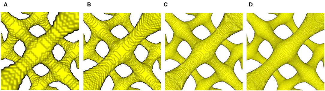
Figure 6. Zoom into center-junction region of most slender geometry G₁₁ scanned with four different voxel resolutions of (A) 60 voxels; (B) 100 voxels; (C) 200 voxels; (D) 300 voxels per unit cell edge length N_v/a_UC.

Skeletonization and Beam Discretization

When analyzing the effect of the different voxel resolutions on the mechanical behavior of the FEM skeleton beam models, the skeletonization, and originating from that, the discretization of the beam elements are further sources of errors. The skeleton of the structure is the one-voxel-wide centerline. It is achieved by surface thinning, as implemented in Fiji. Richert and Huber (2018) discuss different discretization approaches, where the most accurate approach appears to be to construct the beam axis as the connection between the centers of neighboring voxels (1 V/E). However, due to the discrete cubic size of a voxel, this can lead to harsh direction changes of up to 90° between two beam elements (zigzag). Especially for curved ligaments, as found in actual NPG tomography data, this has a great effect. This zigzag skeleton path results in a more compliant mechanical behavior, as shown by Richert and Huber (2018). The other approach is to average over a certain number of voxels. An approach of on average five voxels was tested by Richert and Huber (2018). This solves the issue with the skeleton zigzag on the one hand, but results in a lower number of beam elements per ligament on the other hand and, due to this, the ligament shape may be badly represented. Neckings are averaged out and the macroscopic stiffness and strength is probably overestimated. This is a similar effect as if using a low voxel resolution.

A new approach is introduced in this paper, were the skeleton voxels are fit by a Bezier function. This results in a smooth line, with the start- and end-node being fixed in their position. The Bezier fit is not forced to go exactly through the individual skeleton points of the ligament, so no overshoots arise, as is would be the case for a spline fit. The Bezier approach has the additional advantage that the desired number of equidistant beam elements per ligament can be chosen in dependent of the length and skeleton voxel number of the current ligament. For assuring comparability with the reference FEM beam model, 20 two-node shear flexible Timoshenko beam elements in space (B31) are used (see section Reference FEM Solid and Beam Models). For the boundary conditions (see section Boundary Conditions).

The models for the different discretization approaches based on the Thickness data are shown in Figure 7. The diamond structures analyzed in this paper have initially a straight ligament axis (Figure 7A). By using the discretization of one voxel per beam element (1 V/E) on a 60 voxels scanned structure, kinks are clearly visible in Figure 7B as tilted elements. Also for the 200 voxels scan resolution, the 1 V/E discretization shows kinks (see Figure 7C). This phenomenon is not avoidable due to the discrete voxel size, shape and orientation of the ligaments in space, even for the ideal geometries used in this work. This problem is solved via the newly introduced Bezier fit, which shows nicely aligned beam elements (see Figure 7D). Besides the discretization issues, the diameter overestimation through the Thickness algorithm is clearly visible in all three FEM skeleton beam models (Figures 7B–D), when compared to the reference geometry presented in Figure 7A.

FIGURE 7

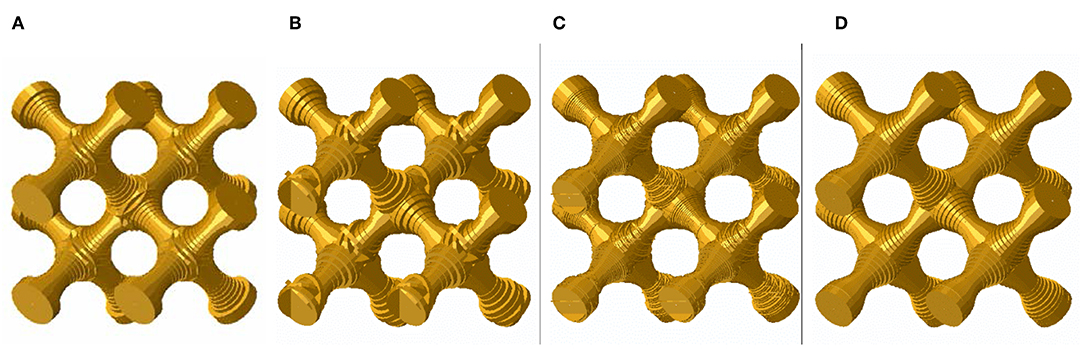
Figure 7. FEM beam models of concave ligament geometry G₁₁: (A) reference FEM beam model; FEM skeleton beam models based on Thickness data with voxel resolution and discretization of (B) 60 V and 1 V/E; (C) 200 V and 1 V/E, (D) 200 V and Bezier representation of the skeleton line.

The FEM skeleton beam model was built from the four different voxel resolutions of the geometry G₁₁ based on the Thickness diameter estimation algorithms. Furthermore, the two different discretization approaches with either each voxel being represented by one beam element (1 V/E), or a Bezier fit (Bez 20 E/L) are applied to the skeleton and diameter data. The results for the Young's modulus are displayed in Figure 8. The values are fit to a simple hyperbolic function $E^{(Th)}=k/(N_v/a_{UC})+E_{\infty }^{(Th)}$, where the parameter $E_{\infty }^{(Th)}$ approximates the Young's modulus for a model with infinite number of voxels N_v/a_UC = ∞, as 590 MPa and 580 MPa for Bezier and 1 V/E discretization, respectively. The percentage deviation from those values is inscribed. The focus is here solely set on the effect of the voxel resolution and the two different beam element discretizations. The deviations to the reference beam model stemming from the diameter estimations are addressed in sections Thickness Analysis and Effect on Mechanical Properties.

FIGURE 8

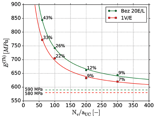
Figure 8. Macroscopic mechanical behavior of the FEM skeleton beam models build from different voxel resolution scans using two different beam element discretization approaches: one skeleton voxel per beam element (1 V/E); Bezier fit of the skeleton points and diameters with 20 elements per ligament (Bez 20 E/L). The values are fit to a simple hyperbolic function $E^{(Th)}=\frac{k}{(N_v/a_{UC})}+E_{\infty }^{(Th)}$. The parameter $E_{\infty }^{(Th)}$ approximates the values for an infinite number of voxels N_v/a_UC, being 590 and 580 MPa for Bezier and 1 V/E discretization, respectively. The percentage deviation from those values is inscribed.

Overall, the 1 VE models show slightly lower Young's modulus values than the Bezier models, and also lower deviations to its asymptotic value of 580 MPa at N_v/a_UC = ∞. As the skeleton is straight in the reference geometry, the effect of the increased compliance caused by the kinks in the ligament axis with the 1 VE discretization is small. For the lowest voxel resolution (60 V) the stiffness is overpredicted by up to 43% while for higher resolution, the accuracy increases. The Young's modulus of the models with a resolution of 200 voxels shows around 10% remaining difference to the predicted value at N_v/a_UC = ∞. Further refinement slowly increases the accuracy, but rapidly increases the computational time. Thus, all further computations will use the voxel resolution of 200 voxels per unit cell edge length N_v/a_UC with the Bezier fit to ensure comparability to the reference structures created with 20 elements per ligament. The remaining uncertainty in the prediction of the mechanical properties is up to 12% due to the voxel resolution and beam element discretization. The resulting voxel edge length of 1/200 (0.005) defines the achievable accuracy limit for the geometrical characterization in the following sections.

Thickness Analysis

This section discusses the geometry derived with the Thickness algorithm (Th) and the Euclidean distance transformation (EDT) from the voxel scan of the underlying reference geometries, given in Table 1. Figure 9A shows the mean-radii 〈r^(.)〉 obtained from averaging over all 20 elements of a ligament normalized by the mean-radius of the reference geometry 〈r^(ref)〉. It can be seen that the deviation of 〈r^(.)〉/〈r^(ref)〉 increases with increasing concavity, independent of the end radius r_end and algorithm used. For the Thickness algorithm, the largest value of 1.2 is comparable to the results of Richert and Huber (2018), where values up to 1.3 have been reported using the mathematically exact ligament geometry as reference. It could be argued that the deviation of 20% in the geometry is still acceptable. However, as showed by Richert and Huber (2018), this causes serious overpredictions in the mechanical stiffness of the ligament by a factor of two. As expected, the data from the EDT show an underprediction for increasing concavity, but the relative deviations are significantly smaller compared to Thickness algorithm.

FIGURE 9

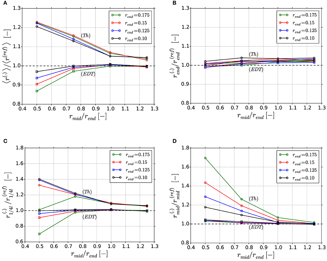
Figure 9. Ratio of computed ligament radii: (A) Ratio of average radius 〈r^(.)〉/〈r^(ref)〉; (B) Ratio of local radius $r_{end}^{(.)}/r_{end}^{(ref)}$; (C) Ratio of local radius $r_{1/4l}^{(.)}/r_{1/4l}^{(ref)}$; (D) Ratio of local radius $r_{mid}^{(.)}/r_{mid}^{(ref)}$. The superscript (.) corresponds to Thickness (Th) or Euclidean distance transform (EDT).

The advantage of the object-oriented-programming is that it enables to locally analyze parameters of individual ligaments at specific positions. Figures 9B–D show selected results for the effect on the local thickness determined in the end, quarter, and middle position of the ligament, respectively. From this series, the strength and weaknesses of each algorithm can discussed. In the overall comparison, the EDT algorithm is of superior accuracy. At the mid and end position, where the tangent of the ligament shape is flat, the diameter is determined with high accuracy. Only in the transition from end to mid position, represented by the quarter positions in Figure 9C, the expected underprediction can be seen in the EDT data. In the worst case that represents the largest diameter change, i.e., structure G₄₁, the deviation is −30%.

For the Thickness algorithm, the local overestimation of the r_mid value increasingly depends also on the absolute radius of the ligament end, the more concave the ligament is. This is a result of the following mechanism: The Thickness algorithm propagates the sizes of the nodal region into the ligament region. Firstly, all skeleton points inside the nodal sphere are assigned with this value R_node ≥ r_end, forming a nodal plateau of constant radius. Secondly, from there the ligament shape assumes a smooth transition from R_node to r_mid. However, in the extreme case of a very thick ligament, the two nodal spheres can even overlap in the mid position of the ligament. This would lead to an extension of the plateau over the whole ligament length. Due to this, the determined radius in the mid-point $r_{mid}^{(Th)}$ can take all possible values from $r_{mid}^{(ref)}$ to R_node.

In the following, we will investigate the impact of the determined geometries on the macroscopic mechanical properties. The question will be addressed in how far the averaged data or the local effects in the geometrical characterization are relevant in terms of the mechanical behavior.

Effect on Mechanical Properties

In section Thickness Analysis, the deviations for the average and local thicknesses are determined for the 16 reference RVEs. Because the diameter enters the moment of inertia by a power of four in the stiffness calculation, the overestimation of the Young's modulus and yield strength is expected to be even higher. To quantify this effect, 16 FEM skeleton beam models are built from the 200 voxel resolution scans (section RVE Size and Voxelization), with a Bezier curve fit to the skeleton axis (section Skeletonization and Beam Discretization). In Figures 10A,B, the macroscopic Young's modulus E and the yield strength σ_y, respectively, obtained from the FEM skeleton beam model are compared to the values from the corresponding reference FEM beam model.

FIGURE 10

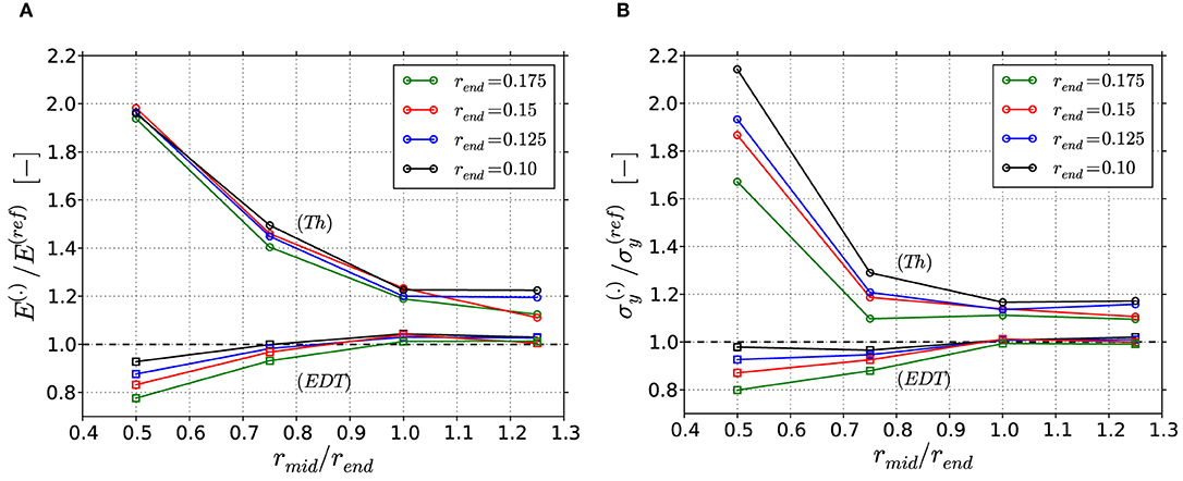
Figure 10. Results of the macroscopic mechanical properties for the FEM skeleton beam models based on the Thickness (Th) algorithm or Euclidean distance transform (EDT), normalized to the results from the reference FEM beam models: (A) Young's modulus E and (B) yield strength σ_y. The superscript (.) corresponds to (Th) or (EDT).

The factor of overestimation of the Young's modulus for the Thickness algorithm, presented in Figure 10A, is similar for structures with same ratio r_mid/r_end, independent of the absolute r_end value. Strongly concave structures show the highest deviations by up to a factor of 2. Tending toward cylindrical and convex structures, the deviation decreases to a factor of 1.2. The trend in the yield strength data in Figure 10B is similar, showing highest overestimations at strongly concave ligaments. With decreasing concavity, the decay is however more emphasized. Furthermore, stronger variations for different r_end values are observed, especially for the concave ligaments. There, smaller r_end values show higher overestimation, ranging from 1.68 to 2.15. The higher sensitivity of the yield strength is caused by the circumstance that the onset of plastic deformation results from the combination of weakest cross-section and applied bending moment, which again depends on the lever acting on this cross-section. In contrast to this, the elastic deformations spread over the whole ligaments and into the junction volumes and are therefore less sensitive to the local geometry (Huber et al., 2014).

It should be noted that cylindrical and convex ligaments show overall the lowest overestimation, which is still about 20% for both macroscopic properties. This is astonishing, as one might imagine that a cylindrical ligament should be perfectly reproduced by the Thickness algorithm. However, this is only true for a cylindrical ligament of infinite length. For the interconnected structure, which contains junction volumes that are larger than the cylindrical ligaments, the overestimation in mechanical properties is due to the mechanism discussed in section Thickness Analysis.

In line with the findings from the geometric analysis presented in Figure 9, the predicted deviations in the macroscopic mechanical properties for the EDT data are much smaller compared those obtained for the Thickness algorithm. The results can be considered accurate for cylindrical and convex shapes while for concave shapes the stiffness and strength are reduced up to 20%. If this is acceptable, the EDT can be used without further correction. It should be noted that stronger concavities or asymmetries as well as non-circular cross-sections can further increase these deviations also for the EDT.

Methods for Thickness Correction

Due to the impact on the mechanical response, we present in the following sections possible correction approaches for both thickness algorithms. The high sensitivity of the mechanical properties on the geometric characterization justifies to use the predicted Young's modulus and yield strength throughout these sections as the relevant measure for the assessment of the quality of each approach.

Smallest Ellipse Approach

Coming from the Biggest Sphere Thickness approach by Hildebrand and Rüegsegger (1997), the idea is to compensate its systematic trend of overestimation by the opposing equivalent, which is the Smallest Sphere approach, discussed by Liu et al. (2014). Between these two extremes, a Smallest Ellipse (SE) approach can be considered, as schematically presented in Figure 11. As input data, the coordinates of the medial axis and the respective Thickness values are used. Each point x along the axis located in a smallest ellipse inscribed into the Thickness data r^(Th), is assigned with the value of the ellipse major axis as the radius r^(SE). The ellipse allows to incorporate some flexibility in the range of radius assignment near the point under investigation. To this end, the linear eccentricity e of the ellipse was determined independently of the geometries defined in Table 1. Approximately 800 ligament geometries were created, reproducing the range of ligament geometries detected by Richert and Huber (2018), including asymmetric ligament shapes. A linear eccentricity of e = 0.75 produced the lowest errors.

FIGURE 11

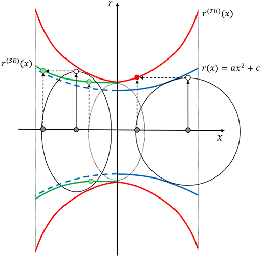
Figure 11. Schematic of the Thickness Biggest Sphere (Th, right half) and Smallest Ellipse (SE, left half) approach sketched in an exemplary ligament section with r(x). Each point x located in a Smallest Ellipse fitted to the Thickness data r^(Th), is assigned with the value of the major axis as the radius r^(SE). The linear eccentricity of the ellipse is fixed to e =0.75.

The obvious drawback of the proposed Smallest Ellipse approach is that the minimum diameter of a ligament is bound to the minimum Biggest Sphere Thickness value. This can be seen in Figure 11, where in the center of the ligament a gap between the minimum radius of the original reference geometry and the reconstructed radius remains. In the nodal areas, the Biggest Sphere Thickness value represents the upper limit, which is correctly reproduced. The algorithm is robust since it does not require any assumption on a model function, parameter bounds, and parameter start values and works for symmetric and asymmetric ligament shapes.

The correction of the geometries via the Smallest Ellipse approach lead to an overall improvement in the predicted macroscopic mechanical properties (see Figure 12). The previously observed overestimation from 1.2 to 2.0 based on the Thickness data (see Figure 10A) is now reduced to an almost constant value between 1.1 and 1.25, i.e., the concave ligaments are most improved. As discussed before, the yield strength shows some stronger sensitivity to the different ligament shape parameters, while the overall improvement is comparable to that of the Young's modulus. In summary, the reconstruction of the ligament shape with the simple Smallest Ellipse approach represents a substantial improvement in comparison to the Thickness data, although some geometrical inaccuracies remain in the thinner region.

FIGURE 12

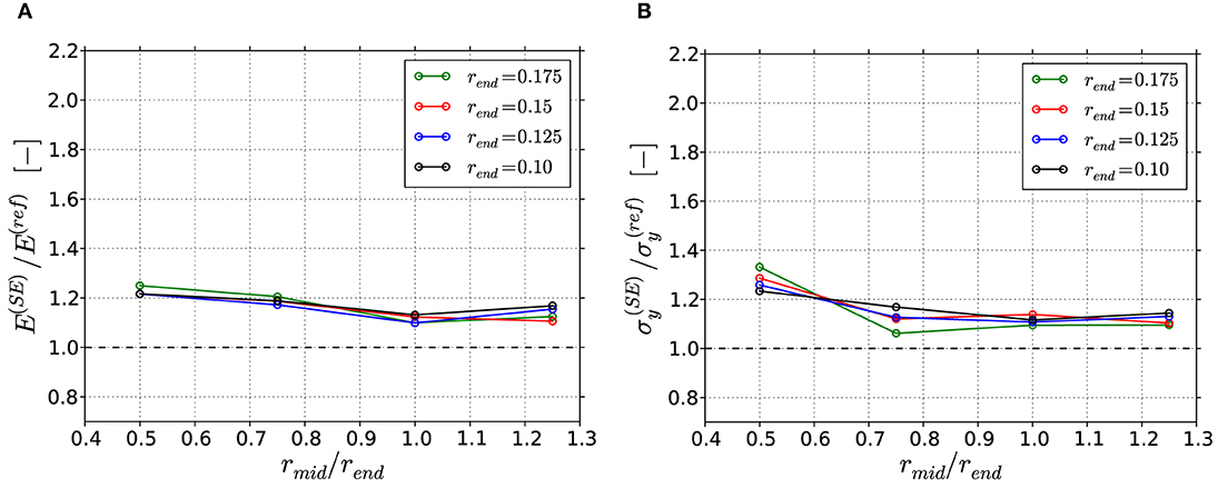
Figure 12. Results of Smallest Ellipse (SE) corrected FEM skeleton beam models normalized to the results from the reference FEM beam models: (A) Macroscopic Young's modulus; (B) Macroscopic yield strength at 1% plastic strain.

Artificial Neural Network Correction Approach

In contrast to the Smallest Ellipse approach, which does not require an assumption with regard to the ligament geometry, computational methods, such as optimization strategies or artificial neural networks can be applied for reconstruction of the original ligament shape. In our case, the ligament shape is limited to symmetric-parabolic shapes, which in principle allows applying both strategies in a straightforward manner. Apart from the drawback of restricting the generality to a certain class of ligament shapes included in the assumed model function, this has the advantage of dealing with the ligament as a whole dataset. Optimization strategies require parameter bounds, parameter start values of the model function. They are furthermore computationally demanding, because the parameter identification must be carried out individually and independently for each ligament. Therefore, we focus on the development of an artificial neural network (ANN).

For details on the ANNs, we refer to Huber (2018) and the literature cited there. For the training of the ANN, the 16 symmetric ligament geometries are used, defined in Table 1. Pattern files are written in the following style: The input vector X consists according to Equation (2) of the radii computed for all elements along the ligament skeleton, normalized by their average, in the form $r^{(.)}(x_i)/\langle r^{(.)}\rangle$, where (.) can be set to any of the three algorithms, namely (Th), (SE), or (EDT). This set of data represents the shape of the ligament from one end to the other end as measured by the corresponding algorithm.

As one further input value, the normalized position 2x_i/l is given, for which the correction factor shall be determined. The output vector Y consists according to Equation (3) of just one value, which is the correct radius divided by the radius determined from the algorithm $r^{(ref)}(x_i)/r^{(.)}(x_i)$ at the position x_i. Because an ANN represents a continuous approximation of the presented data, it is very difficult to predict the steps contained in r^(ref) as shown in Figure 4. Therefore, the prediction of the output is limited to the positions within the triple points. Per ligament, 14 patterns are created, which are related to the 14 element radii for which the correct radius needs to be computed. Each ANN consists of four layers with 21 neurons at the input layer, 15 and 10 neurons in the two hidden layers, and 1 neuron for the output layer and is trained for 10,000 epochs. The resulting mean squared training and validation errors are $MS{E}_T(Th)=2.37·10^{-5}$ and $MS{E}_V(Th)=1.87·10^{-4}$; $MS{E}_T(SE)=8.82·10^{-6}$ and $MS{E}_V(SE)=8.44·10^{-5}$; $MS{E}_T(EDT)=1.73·10^{-5}$ and $MS{E}_V(EDT)=1.89·10^{-4}$; respectively.

$\begin{array}{ll}\text{X}=\left\{\frac{r^{(.)}(x_1)}{\langle r^{(.)}\rangle },\frac{r^{(.)}(x_2)}{\langle r^{(.)}\rangle },\dots ,\frac{r^{(.)}(x_{20})}{\langle r^{(.)}\rangle },\frac{2x_i}{l}\right\}& (2)\end{array}$

$\begin{array}{ll}\text{Y}=\left\{\frac{r^{(ref)}(x_i)}{r^{(.)}(x_i)}\right\}& (3)\end{array}$

Indicated by the very low training and validation error, the reconstruction of the correct ligament shape seems to be a simple task for the ANN. The ANNs are able to determine the original ligament radius within one voxel accuracy, independent by which algorithm the input data are provided.

To validate the generalization capability of the trained ANNs, three new validation geometries are generated within the range of the existing 16 geometries. They are defined with r_end = 0.1375 and r_mid/r_end = [0.625, 0.875, 1.125]. The geometries of the three validation examples are shown in Figure 13. The degree of the remaining deviations is illustrated by 1 voxel- (±0.5 v) and 2 voxel-wide (±1 v) bands. The radii determined along the ligaments is within or very close to the 2-voxel wide band range for all three validation geometries and three ANN types. This corresponds to plus-minus one voxel, which is the limit for the accuracy defined by the voxel resolution. Only for the corrected Thickness data of strongly concave ligament in Figure 13A, the determined values are far outside the 2-voxel wide band.

FIGURE 13

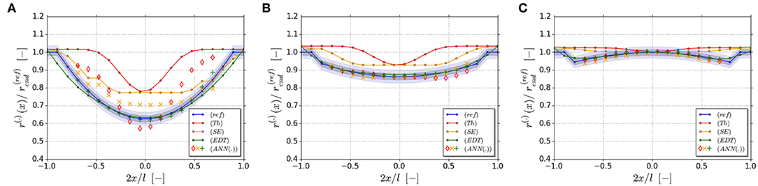
Figure 13. Validation cases including the correct geometry r^(ref), the Thickness result r^(Th), the Smallest Ellipse result r^(SE), the EDT result r^(EDT), and the ANN-reconstructed geometries r^(ANN(Th)), r^(ANN(SE)), r^(ANN(EDT)) for r_end = 0.1375. The degree of the deviations is illustrated by 1 voxel- (±0.5 v) and 2 voxel-wide (±1 v) bands: (A) r_mid/r_end = 0.625; (B) r_mid/r_end = 0.875; (C) r_mid/r_end = 1.125.

If the Thickness data are pre-processed with the Smallest Ellipse algorithm, the accuracy improves significantly also for this difficult case. The ANN is now able to achieve accuracies, which are within the theoretical resolution limit of the voxel discretization and comparable to the results of the EDT (Figures 13A–C). This results from the capability of the ANN to memorize the relationship between ligament shapes and their corrections as whole and smoothly interpolate this relationship for untrained geometries. Due to this, the ANN approach has superior performance compared to the local Smallest Ellipse approach, discussed in the previous section, which cannot fully recover the information in the thinnest part of the ligament. The drawback is however that this method is so far limited to symmetric ligaments. For further evaluations of actual tomography data in the parameter space of $r_{sym}^{*}$ and $r_{asym}^{*}$, as found by Richert and Huber (2018), the incorporation of a linear gradient according to Equation (1) is required. With this, asymmetric ligaments can be represented, as they occur with high probability in real NPG. Motivated by the promising results presented in this section, such an extension will be scope of future work.

As for the resulting mechanical behavior, very small deviations of maximum 10% are observed for the 16 trained geometries for both Young's modulus and yield strength. Also the three additional validation examples are well-predicted by the ANN with the very same accuracy, supposed the Thickness data are improved by the Smallest Ellipse approach before feeding the data to the ANN. It is remarkable that, despite some remaining error in the geometry reconstruction, resulting errors in the mechanical properties are negligible. The reason for this is that the ANN in average determines the ligament shape correctly with perhaps some small over- and under-predictions in different regions of the ligament. In contrast to that, the Thickness algorithm and the reconstruction via the Smallest Ellipse approach systematically overestimate the geometry and therefore the mechanical properties are biased to higher values.

Application To Experimental Tomography Data

To test the methods presented in section Methods for Thickness Correction beyond the 16 idealized diamond structures, the NPG tomography data set of Hu et al. (2016) is used, which stems from a nanoporous gold sample with nominally 400 nm average ligament diameter. Three FEM skeleton beam models are generated based on the Thickness, EDT and furthermore Smallest Ellipse corrected data of the NPG tomography, as described in section FEM Skeleton Beam Models. The ANN approach is not applicable in its present form, as it requires an extension toward more general shapes. The mesh of the reference Solid model consisting of 10-node tetrahedral elements (C3D10) was provided by Hu et al. (2016). For both types of models, symmetry boundary conditions are used and a compressive loading in z-direction is applied. In this way, the results give an additional insight about the effect for a more commonly used boundary condition and a realistic, aperiodic microstructure. The resulting macroscopic stress-strain behaviors are plotted in Figure 14; the inserts clearly show the differences in the resulting beam models relative to the solid model, where the black line shows the traced outline of the solid model.

FIGURE 14

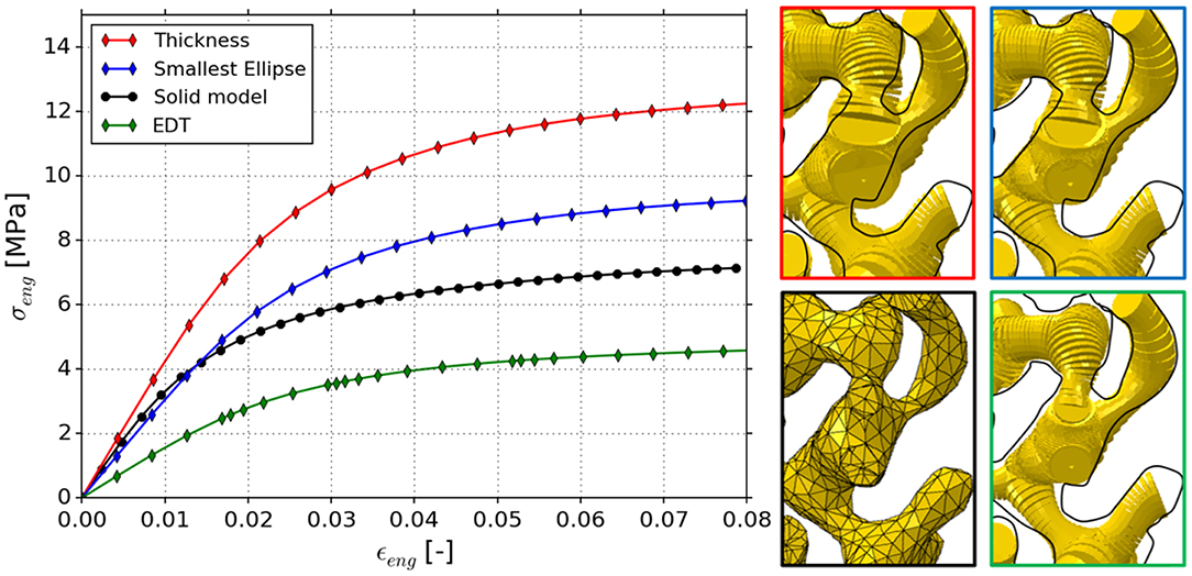
Figure 14. Stress strain curves of NPG tomography of Hu et al. (2016) modeled as FEM solid model and predictions from FEM skeleton beam models based on Thickness, Smallest Ellipse, and EDT diameter information. Inserts show regions of interest for comparison of the determined geometries.

The macroscopic Young's moduli and yield strengths at 1% plastic strain are computed as 432 and 10.0 MPa (Thickness); 310 and 7.5 MPa (Smallest Ellipse); 160 and 3.7 MPa (EDT), respectively. For comparison, the Young's modulus and yield strength of the FEM solid model was computed as 370 and 5.5 MPa. Consistent with the trend observed for the idealized diamond structures, the model based on Thickness and EDT diameter information show the highest and lowest values, respectively. From the idealized diamond structures, we computed ratios (Thickness/EDT) in the average diameter ranging from 1.05 (highest convexity) to 1.4 (highest concavity). The corresponding ratios in the predicted mechanical properties are ranging from 1.2 to 2.5 (Young's modulus) and 1.2 to 2.7 (yield strength). For the NPG tomography, the ligament diameter distribution resulting from the Thickness and EDT algorithms showed a ratio in the average ligament diameter of 1.3 (see section Methodology and Figure 1). As shown in Figure 14, the (Thickness/EDT) ratio computed for the macroscopic mechanical properties are 2.7 (Young's modulus) and 2.7 (yield strength). Therefore, geometry and property ratios for the real material are close to or above the upper limits found for the idealized diamond structures. This is reasonable, because the diamond structure exhibits straight skeleton lines and symmetric ligament profiles while the skeleton paths in the NPG sample are more randomized and ligament profiles are strongly asymmetric, as reported by Richert and Huber (2018). Therefore, the ligaments show additional gradients along their axis—such gradients are found to be the source of error in both algorithms, Thickness and EDT.

Furthermore, the resulting Young's modulus of the EDT beam model is only 43% of the solid model. This confirms the expectation by Richert and Huber (2018) that the FEM Solid model should be stiffer and stronger than the FEM skeleton beam model, as in the latter, the stiffening and strengthening effect of the nodal mass (Jiao and Huber, 2017b) is not yet accounted for.

Conclusions and Outlook

While the accurate determination of the thickness of geometrical features from 2D images is straight forward, the situation changes dramatically for 3D structures. Various algorithms exist, but each has its specific drawbacks regarding implementation, computational cost, or accuracy. The Thickness algorithm by Hildebrand and Rüegsegger (1997) is the most commonly used algorithm. This is usually done without an assessment of the error, because information about the correct thickness of the structures under investigation is not available. A study by Richert and Huber (2018) of typical ligament shapes identified from 3D FIB tomography data of NPG revealed that the error in the measured geometry can reach values up to 30%. The overestimated thickness data lead to an overestimation of the mechanical stiffness by a factor of two and more. Although an implementation of the 3D Euclidean distance transformation (EDT) is for example available in the Plugin TANGO, this algorithm has so far not been used in 3D analysis. In contrast to the Thickness algorithm, it tends to underpredict the diameter for curved shapes. A first comparison of both algorithms with tomography data of NPG revealed a difference in the computed average ligament diameter of 30%. This and the detailed results obtained on the local radii for the different algorithms highlight how important it is to understand the individual algorithm used and what the produced data represent in relation to the measure of interest. This is particularly an issue when pooling data from various sources making use of different algorithms.

To provide RVEs with well-defined geometries, this work is based on idealized model structures consisting of ligaments with circular cross-sections and smooth parabolic-spherical shape, organized in a diamond structure. Sixteen high-resolution voxel models and finite element models are provided, covering the relevant shapes from concave to convex ligaments. These models serve as reference for the error assessment for both, the determined geometry and the elastic-plastic mechanical properties along the thickness determination and correction chain. Furthermore, the provided test structures can be used for validation of any newly developed algorithm for the determination or correction of thickness information from voxel data.

To decouple this study from the known effect that FEM beam models show a more compliant and less strong macroscopic stress-strain behavior compared to FEM solid models, the differences in both properties are computed for each geometry. As expected, the FEM beam model is more compliant compared to the FEM solid model. The data show an increasing deviation for increasing mid to end radius ratio while the ligament size has only a marginal effect. In contrast to this, the yield strength distributes below and above those of the FEM solid model. This surprising result leads to the conclusion that the stress-strain curve computed by Richert and Huber (2018) must not necessarily fall below the curve predicted by the FEM solid model, after the geometry is corrected, because a newly developed nodal correction for these ligament shapes may not necessarily increase the strength.

An investigation of the sensitivity with regard to the voxel resolution revealed that the predicted mechanical stiffness is significantly overestimated with decreasing voxel number. For the most filigree structures and a resolution of 60 voxels per unit cell length, the error reaches up to 30% in comparison to a resolution of 300 voxels. Increasing the resolution to 200 voxels reduces the error to 3%.

Applying the Thickness algorithm to the data with 200 voxels resolution yielded largest overestimations of 20% in the average radius and 70% in the radius in the middle of the ligament. The impact on the Young's modulus and yield strength is up to 100% overestimation for concave shapes. This is not as high as predicted in the single ligament study by Richert and Huber (2018), but is still inacceptable. The Euclidean distance transformation resulted in an underprediction in the macroscopic mechanical properties of up to 20% for concave ligaments.

In view of these results, two approaches for correction of the computed thickness are proposed. A Smallest Ellipse correction approach, which could be interpreted as counterpart of the Biggest Sphere Thickness algorithm, allows reducing the error in Young's modulus to 20% and in yield strength to 30% for all ligament shapes. Secondly, using patterns consisting of estimated thickness information from Thickness, Smallest Ellipse, Euclidean distance transformation algorithm, and original ligament shapes, artificial neural networks were trained. It could be shown that the accuracies achieved for most cases are within a few voxels. The resulting deviations in the mechanical properties are within few percent, even for untrained validation patterns. This demonstrates the big potential of ANNs to accurately approximate complex non-linear relationships as whole. Even a correct reconstruction is possible for data for which the input information is incomplete in terms of the original ligament shape. However, relative to the ANN corrected Thickness data, the accuracy can be significantly increased by presenting the data from the Smallest Ellipse algorithm. This shows that it is advisable to reduce the complexity of the problem as far as possible by using existing algorithms or estimates, even if they are of limited accuracy. Such strategies have been successfully applied before and the outcome of this work emphasizes once more the importance of incorporation of a priori knowledge in the preparation of the ANN definition and pattern generation when high accuracy is a requirement. This is particularly important for solving highly non-linear and complex inverse problems (Huber and Tsakmakis, 1999, 2001; Tyulyukovskiy and Huber, 2006).

An obvious drawback of the ANN approach is that it must be trained for the parameter space of possible shapes to be identified. This means that for the evaluation of tomography data in the parameter space of $r_{sym}^{*}$ and $r_{asym}^{*}$, as found by Richert and Huber (2018), requires an expansion by a linear gradient along the ligament axis or the incorporation of even more general shapes. In addition, the results of the Thickness and EDT algorithms should be critically evaluated with respect to effects from non-circular cross-sections that might occur in real samples.

Thus, future research should be directed toward approaches that provide sufficient geometrical accuracy for a large range of possible ligament geometries, where the accuracy should always be evaluated in view of the predicted mechanical properties.

Finally, the Thickness, Smallest Ellipse, and EDT algorithms are applied to the experimental NPG tomography data set of Hu et al. (2016). The average diameters and predicted stress-strain curves consistently showed Thickness to EDT ratios at the upper limit of the range computed for the idealized diamond structures. This is consistent with the finding that gradients in the ligament diameter along the axis are responsible for systematic over- and underestimation by the algorithms. Obviously, this effect is enhanced by the random nature and strong asymmetry of real ligaments. Furthermore, the stress-strain curve of the solid model lies in between the Thickness and EDT prediction. While the overprediction based on Thickness data confirms the result reported by Richert and Huber (2018), the EDT curve being significantly below the result of the FEM solid model now opens the perspective for an implementation of a physically meaningful nodal correction in the FEM beam model.

Author Contributions

CR and NH conceptualized, designed the study, and wrote and revised the manuscript. NH created the geometries, FEM solid and FEM beam models, and coded the Python scripts for voxel scanning. CR analyzed the voxel scans, carried out the FEM skeleton beam models. AO developed the Smallest Ellipse approach and carried out the thickness correction using this method. CR developed the ANN for thickness correction, analyzed the errors of all methods in terms of geometry and mechanical properties.

Funding

This work was funded by the Deutsche Forschungsgemeinschaft (DFG, German Research Foundation)—Projektnummer 192346071—SFB 986.

Conflict of Interest

The authors declare that the research was conducted in the absence of any commercial or financial relationships that could be construed as a potential conflict of interest.

Acknowledgments

Kaixiong Hu and Erica T. Lilleodden are acknowledged for making the FIB tomography data set and the FEM solid model of NPG available.

Supplementary Material

The Supplementary Material for this article can be found online at: https://www.frontiersin.org/articles/10.3389/fmats.2019.00327/full#supplementary-material

References

Abaqus (2014). Theory Manual. Providence, RI: Dassault Systèmes.

Google Scholar

Almhdie-Imjabber, A., Hambli, R., Touvier, J., Rozenbaum, O., Lespessailles, E., and Jennane, R. (2014). Mechanical assessment of trabecular bone stiffness using hybrid skeleton and finite element analysis. Comput. Methods Biomech. Biomed. Eng. 4, 352–359. doi: 10.1080/21681163.2014.944355

CrossRef Full Text | Google Scholar

Arganda-Carreras, I., Fernández-González, R., Muñoz-Barrutia, A., and Ortiz-De-Solorzano, C. (2010). 3D reconstruction of histological sections: application to mammary gland tissue. Microsc. Res. Tech. 73, 1019–1029. doi: 10.1002/jemt.20829

PubMed Abstract | CrossRef Full Text | Google Scholar

Ashby, M., Evans, T., Fleck, N. A., Hutchinson, J., Wadley, H., and Gibson, L. J. (2000). Metal Foams: A Design Guide. Oxford: Butterworth-Heinemann.

Google Scholar

Badwe, N., Chen, X., and Sieradzki, K. (2017). Mechanical properties of nanoporous gold in tension. Acta. Mater. 129, 251–258. doi: 10.1016/j.actamat.2017.02.040

CrossRef Full Text | Google Scholar

Day, J. S., Ding, M., Odgaard, A., Sumner, D. R., Hvid, I., and Weinans, H. (2000). Parallel plate model for trabecular bone exhibits volume fraction-dependent bias. Bone 27, 715–720. doi: 10.1016/S8756-3282(00)00371-9

PubMed Abstract | CrossRef Full Text | Google Scholar

Diebels, S., and Steeb, H. (2002). The size effect in foams and its theoretical and numerical investigation. Proc. R. Soc. Lond. A 458, 2869–2883. doi: 10.1098/rspa.2002.0991

CrossRef Full Text | Google Scholar

Dillard, T., N'guyen, F., Maire, E., Salvo, L., Forest, S., Bienvenu, Y., et al. (2005). 3D quantitative image analysis of open-cell nickel foams under tension and compression loading using X-ray microtomography. Philos. Mag. 85, 2147–2175. doi: 10.1080/14786430412331331916

CrossRef Full Text | Google Scholar

Doube, M., Klosowski, M. M., Arganda-Carreras, I., Cordelières, F. P., Dougherty, R. P., Jackson, J. S., et al. (2010). BoneJ: free and extensible bone image analysis in ImageJ. Bone 47, 1076–1079. doi: 10.1016/j.bone.2010.08.023

PubMed Abstract | CrossRef Full Text | Google Scholar

Dougherty, R., and Kunzelmann, K.-H. (2007). Computing local thickness of 3D structures with ImageJ. MAM 13, 1678–1679. doi: 10.1017/S1431927607074430

CrossRef Full Text | Google Scholar

Düster, A., Parvizian, J., Yang, Z., and Rank, E. (2008). The finite cell method for three-dimensional problems of solid mechanics. Comput. Methods Appl. Mech. Eng. 197, 3768–3782. doi: 10.1016/j.cma.2008.02.036

CrossRef Full Text | Google Scholar

Düster, A., Rank, E., and Szabó, B. A. (2017). “The p-version of the finite element and finite cell methods,” in Encyclopedia of Computational Mechanics Second Edition, eds E. Stein, R. de Borst, and T. J. R. Hughes (Chichester; Hoboken, NJ: John Wiley and Sons, Ltd.), 1–35. doi: 10.1002/9781119176817.ecm2003g

CrossRef Full Text | Google Scholar

Gibson, L. J., and Ashby, M. F. (1997). Cellular Solids. Cambridge: Cambridge University Press.

PubMed Abstract | Google Scholar

Gnegel, S., Li, J., Mameka, N., Huber, N., and Düster, A. (2019). Numerical investigation of polymer coated nanoporous gold. Materials 12:2178. doi: 10.3390/ma12132178

PubMed Abstract | CrossRef Full Text | Google Scholar

Hildebrand, T., and Rüegsegger, P. (1997). A new method for the model-independent assessment of thickness in three-dimensional images. J. Microsc. 185, 67–75. doi: 10.1046/j.1365-2818.1997.1340694.x

CrossRef Full Text | Google Scholar

Hu, K. (2017). Micromechanical and three-dimensional microstructural characterization of nanoporous gold-epoxy composites (dissertation). Hamburg: Hamburg University of Technology, Germany.

Google Scholar

Hu, K., Ziehmer, M., Wang, K., and Lilleodden, E. T. (2016). Nanoporous gold: 3D structural analyses of representative volumes and their implications on scaling relations of mechanical behaviour. Philos. Mag. 96, 3322–3335. doi: 10.1080/14786435.2016.1222087

CrossRef Full Text | Google Scholar

Huber, N. (2018). Connections between topology and macroscopic mechanical properties of three-dimensional open-pore materials. Front. Mater. 5:5801. doi: 10.3389/fmats.2018.00069

CrossRef Full Text | Google Scholar

Huber, N., and Tsakmakis, C. (1999). Determination of constitutive properties from spherical indentation data using neural networks. Part I: the case of pure kinematic hardening in plasticity laws. J. Mech. Phys. Solids 47, 1569–1588. doi: 10.1016/S0022-5096(98)00109-4

CrossRef Full Text | Google Scholar

Huber, N., and Tsakmakis, C. (2001). A neural network tool for identifying the material parameters of a finite deformation viscoplasticity model with static recovery. Comput. Methods Appl. Mech. Eng. 191, 353–384. doi: 10.1016/S0045-7825(01)00278-X

CrossRef Full Text | Google Scholar

Huber, N., Viswanath, R. N., Mameka, N., Markmann, J., and Weißmüller, J. (2014). Scaling laws of nanoporous metals under uniaxial compression. Acta. Mater. 67, 252–265. doi: 10.1016/j.actamat.2013.12.003

CrossRef Full Text | Google Scholar

Jiao, J., and Huber, N. (2017a). Deformation mechanisms in nanoporous metals: effect of ligament shape and disorder. Comput. Mater. Sci. 127, 194–203. doi: 10.1016/j.commatsci.2016.10.035

CrossRef Full Text | Google Scholar

Jiao, J., and Huber, N. (2017b). Effect of nodal mass on macroscopic mechanical properties of nanoporous metals. Int. J. Mech. Sci. 134, 234–243. doi: 10.1016/j.ijmecsci.2017.10.011

CrossRef Full Text | Google Scholar

Jin, H.-J., Kurmanaeva, L., Schmauch, J., Rösner, H., Ivanisenko, Y., and Weissmüller, J. (2009). Deforming nanoporous metal: role of lattice coherency. Acta. Mater. 57, 2665–2672. doi: 10.1016/j.actamat.2009.02.017

CrossRef Full Text | Google Scholar

Kinney, J. H., Marshall, G. W., Marshall, S. J., and Haupt, D. L. (2001). Three-dimensional imaging of large compressive deformations in elastomeric foams. J. Appl. Polym. Sci. 80, 1746–1755. doi: 10.1002/app.1269

CrossRef Full Text | Google Scholar

Lee, T. C., Kashyap, R. L., and Chu, C. N. (1994). Building skeleton models via 3-D medial surface axis thinning algorithms. CVGIP Models Image Proc. 56, 462–478. doi: 10.1006/cgip.1994.1042

CrossRef Full Text | Google Scholar

Liu, L.-Z., and Jin, H.-J. (2017). Scaling equation for the elastic modulus of nanoporous gold with “fixed” network connectivity. Appl. Phys. Lett. 110:211902. doi: 10.1063/1.4984108

CrossRef Full Text | Google Scholar

Liu, Y., Jin, D., Li, C., Janz, K. F., Burns, T. L., Torner, J. C., et al. (2014). A robust algorithm for thickness computation at low resolution and its application to in vivo trabecular bone CT imaging. IEEE Trans. Bio-med. Eng. 61, 2057–2069. doi: 10.1109/TBME.2014.2313564

PubMed Abstract | CrossRef Full Text | Google Scholar

Maier, J., Black, M., Bonaretti, S., Bier, B., Eskofier, B., Choi, J.-H., et al. (2017). Comparison of different approaches for measuring tibial cartilage thickness. J. Integr. Bioinform. 14, 1–10. doi: 10.1515/jib-2017-0015

PubMed Abstract | CrossRef Full Text | Google Scholar

Mangipudi, K. R., Epler, E., and Volkert, C. A. (2016). Topology-dependent scaling laws for the stiffness and strength of nanoporous gold. Acta Mater. 119, 115–122. doi: 10.1016/j.actamat.2016.08.012

CrossRef Full Text | Google Scholar

McCue, I., Stuckner, J., Murayama, M., and Demkowicz, M. J. (2018). Gaining new insights into nanoporous gold by mining and analysis of published images. Sci. Rep. 8:6761. doi: 10.1038/s41598-018-25122-3

PubMed Abstract | CrossRef Full Text | Google Scholar

Miehe, C., and Koch, A. (2002). Computational micro-to-macro transitions of discretized microstructures undergoing small strains. Arch. Appl. Mech. 72, 300–317. doi: 10.1007/s00419-002-0212-2

CrossRef Full Text | Google Scholar

Nachtrab, S., Kapfer, S., Arns, C. H., Madadi, M., Mecke, K., and Schröder-Turk, G. (2011). Morphology and linear-elastic moduli of random network solids. Adv. Mater. 23:2633. doi: 10.1002/adma.201004094

PubMed Abstract | CrossRef Full Text | Google Scholar

Nieh, T., Kinney, J., Wadsworth, J., and Ladd, A. (1998). Morphology and elastic properties of aluminum foams produced by a casting technique. Script. Mater. 38, 1487–1494. doi: 10.1016/S1359-6462(98)00090-6

CrossRef Full Text | Google Scholar

Nieh, T. G., Higashi, K., and Wadsworth, J. (2000). Effect of cell morphology on the compressive properties of open-cell aluminum foams. Mater. Sci. Eng. A 283, 105–110. doi: 10.1016/S0921-5093(00)00623-7

CrossRef Full Text | Google Scholar

Ollion, J., Cochennec, J., Loll, F., Escudé, C., and Boudier, T. (2013). TANGO: a generic tool for high-throughput 3D image analysis for studying nuclear organization. Bioinformatics 29, 1840–1841. doi: 10.1093/bioinformatics/btt276

PubMed Abstract | CrossRef Full Text | Google Scholar

Parvizian, J., Düster, A., and Rank, E. (2007). Finite cell method. Comput. Mech. 41, 121–133. doi: 10.1007/s00466-007-0173-y

CrossRef Full Text | Google Scholar

Pia, G., and Delogu, F. (2015). Nanoporous au: statistical analysis of morphological features and evaluation of their influence on the elastic deformation behavior by phenomenological modeling. Acta Mater. 85, 250–260. doi: 10.1016/j.actamat.2014.11.040

CrossRef Full Text | Google Scholar

Richert, C., and Huber, N. (2018). Skeletonization, geometrical analysis, and finite element modeling of nanoporous gold based on 3d tomography data. Metals 8:282. doi: 10.3390/met8040282

CrossRef Full Text | Google Scholar

Roschning, B., and Huber, N. (2016). Scaling laws of nanoporous gold under uniaxial compression: effects of structural disorder on the solid fraction, elastic poisson's ratio, young's modulus and yield strength. J. Mech. Phys. Solids 92, 55–71. doi: 10.1016/j.jmps.2016.02.018

CrossRef Full Text | Google Scholar

Rösner, H., Parida, S., Kramer, D., Volkert, C. A., and Weissmüller, J. (2007). Reconstructing a nanoporous metal in three dimensions: an electron tomography study of dealloyed gold leaf. Adv. Eng. Mater. 9, 535–541. doi: 10.1002/adem.200700063

CrossRef Full Text | Google Scholar

Schindelin, J., Arganda-Carreras, I., Frise, E., Kaynig, V., Longair, M., Pietzsch, T., et al. (2012). Fiji: an open-source platform for biological-image analysis. Nat. Methods 9, 676–682. doi: 10.1038/nmeth.2019

PubMed Abstract | CrossRef Full Text | Google Scholar

Soyarslan, C., Argeso, H., and Bargmann, S. (2018b). Skeletonization-based beam finite element models for stochastic bicontinuous materials: application to simulations of nanoporous gold. J. Mater. Res. 33, 3371–3382. doi: 10.1557/jmr.2018.244

CrossRef Full Text | Google Scholar

Soyarslan, C., Bargmann, S., Pradas, M., and Weissmüller, J. (2018a). 3D stochastic bicontinuous microstructures: generation, topology and elasticity. Acta Mater. 149, 326–340. doi: 10.1016/j.actamat.2018.01.005

CrossRef Full Text | Google Scholar

Soyarslan, C., Husser, E., and Bargmann, S. (2017). Effect of surface elasticity on the elastic response of nanoporous gold. J. Nanomech. Micromech. 7:4017013. doi: 10.1061/(ASCE)NM.2153-5477.0000126

CrossRef Full Text | Google Scholar

Stuckner, J., Frei, K., McCue, I., Demkowicz, M. J., and Murayama, M. (2017). AQUAMI: an open source python package and GUI for theautomatic quantitative analysis of morphologically complex multiphase materials. Comput. Mater. Sci. 139, 320–329. doi: 10.1016/j.commatsci.2017.08.012

CrossRef Full Text | Google Scholar

Stukowski, A. (2010). Visualization and analysis of atomistic simulation data with OVITO - the open visualization tool. Model. Simul. Mater. Sci. Eng. 18:015012. doi: 10.1088/0965-0393/18/1/015012

CrossRef Full Text | Google Scholar

Sun, X.-Y., Xu, G.-K., Li, X., Feng, X.-Q., and Gao, H. (2013). Mechanical properties and scaling laws of nanoporous gold. J. Appl. Phys. 113:023505. doi: 10.1063/1.4774246

CrossRef Full Text | Google Scholar

Tyulyukovskiy, E., and Huber, N. (2006). Identification of viscoplastic material parameters from spherical indentation data: part I. Neural Netw. J. Mater. Res. 21, 664–676. doi: 10.1557/jmr.2006.0076

CrossRef Full Text | Google Scholar

Witkowska, A., Alibhai, A., Hughes, C., Price, J., Klisch, K., Sturrock, C. J., et al. (2014). Computed tomography analysis of guinea pig bone: architecture, bone thickness and dimensions throughout development. PeerJ 2:e615. doi: 10.7717/peerj.615

PubMed Abstract | CrossRef Full Text | Google Scholar

Ziehmer, M., Hu, K., Wang, K., and Lilleodden, E. T. (2016). A principle curvatures analysis of the isothermal evolution of nanoporous gold: quantifying the characteristic length-scales. Acta Mater. 120, 24–31. doi: 10.1016/j.actamat.2016.08.028

CrossRef Full Text | Google Scholar