Strain localization and shear band propagation in ductile materials

1. Introduction

When a ductile material is brought to an extreme strain state through a uniform loading process, the deformation may start to localize into thin and planar bands, often arranged in regular lattice patterns. This phenomenon is quite common and occurs in many materials over a broad range of scales: from the kilometric scale in the earth crust (Kirby, 1985), down to the nanoscale in metallic glass (Yang et al., 2005), see the examples, reported in Figure 1.

FIGURE 1

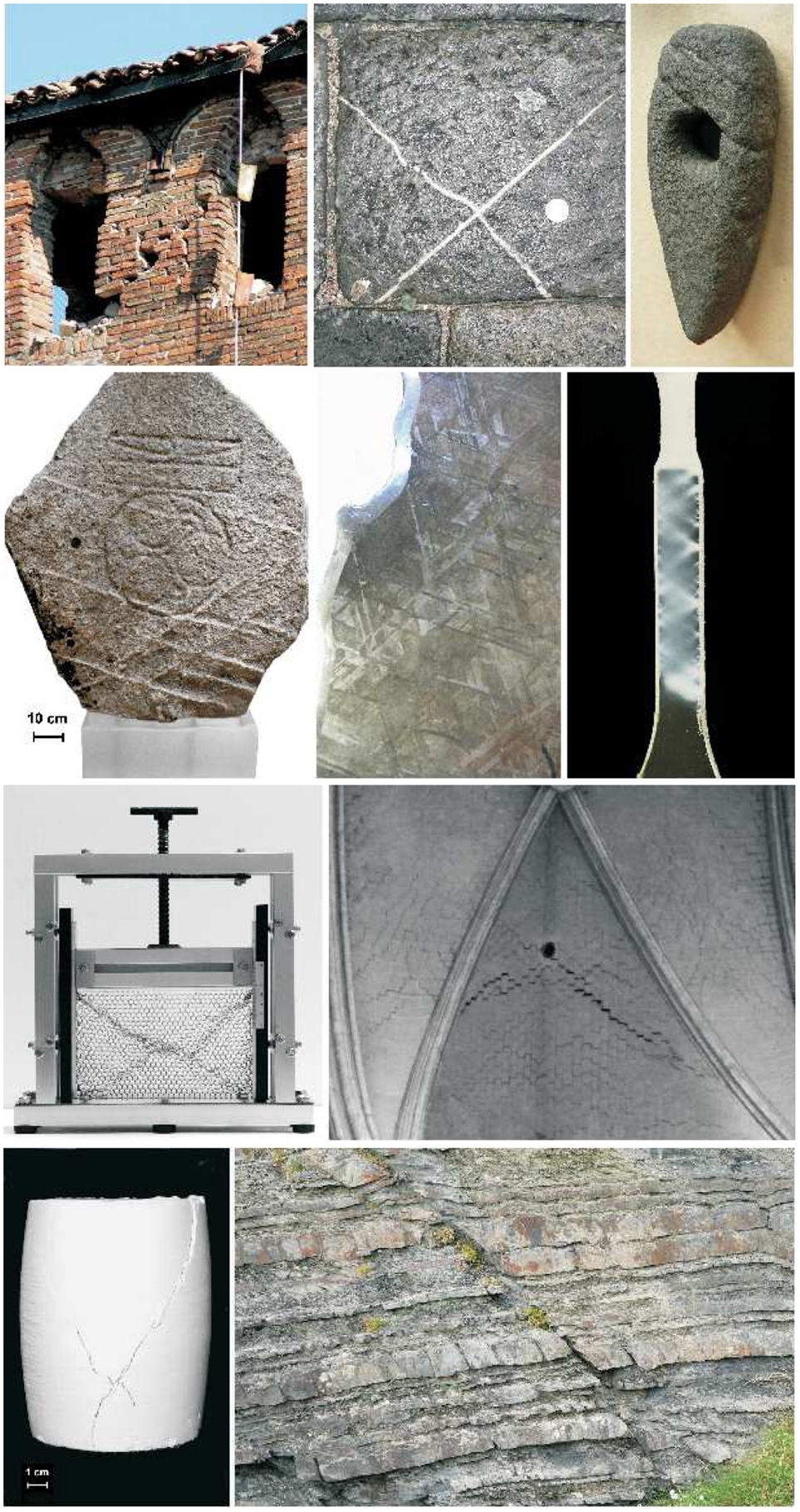
Figure 1. Examples of strain localization. From left to right, starting from the upper part: A merlon in the Finale Emilia castle failed (during the Emilia earthquake on May 20, 2012) in compression with a typical “X-shaped” deformation band pattern (bricks are to be understood here as the microstructure of a composite material). A sedimentary rock with the signature of an “X-shaped” localization band (infiltrated with a different mineral after formation). A stone axe from a British Island (Museum of Edinburgh) evidencing two parallel localization bands and another at a different orientation. A runestone (Museum of Edinburgh) with several localized deformation bands, forming angles of approximately 45° between each other. A polished and etched section of an iron meteorite showing several alternate bands of kamacite and taenite. Deformation bands in a strip of unplasticized poly(vinyl chloride) (uPVC) pulled in tension and eventually evolving into a necking. An initially regular hexagonal disposition of drinking straws subject to uniform uniaxial strain has evolved into an “X-shaped” localization pattern. A fracture prevails on a regularly distributed network of cracks in a vault of the Amiens dome. “X-shaped” localization bands in a kaolin sample subject to vertical compression and lateral confining pressure. A thin, isolated localization band in a sedimentary layered rock (Silurian formation near Aberystwyth).

After localization, unloading typically¹ occurs in the material outside the bands, while strain quickly evolves inside, possibly leading to final fracture (as in the examples shown in Figure 2, where the crack lattice is the signature of the initial shear band network²) or to a progressive accumulation of deformation bands (as, for instance, in the case of the drinking straws, or of the iron meteorite, or of the uPVC sample shown in Figure 1, or in the well-known case of granular materials, where fracture is usually absent and localization bands are made up of material at a different relative density, Gajo et al., 2004).

FIGURE 2

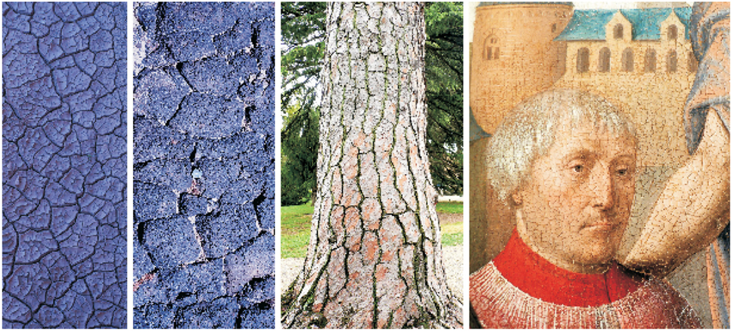
Figure 2. Regular patterns of localized cracks as the signature of strain localization lattices. From left to right: Dried mud; Lava cracked during solidification (near Amboy crater); Bark of a maritime pine (Pinus pinaster); Cracks in a detail of a painting by J. Provost (“Saint Jean-Baptiste,” Valenciennes, Musée des Beaux Arts).

It follows from the above discussion that as strain localization represents a prelude to failure of ductile materials, its mechanical understanding paves the way to the innovative use of materials in extreme mechanical conditions. For this reason, shear bands have been the focus of a thorough research effort. In particular, research initiated with pioneering works by Hill (1962), Nadai (1950), Mandel (1962), Prager (1954), Rice (1977), Thomas (1961), and developed – from theoretical point of view – into two principal directions, namely, the dissection of the specific constitutive features responsible for strain localization in different materials (for instance, as related to the microstructure, Danas and Ponte Castaneda, 2012; Bacigalupo and Gambarotta, 2013; Tvergaard, 2014) and the struggle for the overcoming of difficulties connected with numerical approaches [reviews have been given by Needleman and Tvergaard (1983) and Petryk (1997)]. Although these problems are still not exhausted, surprisingly, the most important questions have only marginally been approached and are therefore still awaiting explanation. These are as follows: (i) Why are shear bands a preferred mode of failure for ductile materials? (ii) Why do shear bands propagate rectilinearly under mode II, while cracks do not? (iii) How does a shear band interact with a crack or with a rigid inclusion? (iv) Does a stress concentration exist at a shear band tip? (v) How does a shear band behave under dynamic conditions?

The only systematic³ attempt to solve these problems seems to have been a series of works by Bigoni and co-workers, based on the perturbative approach to shear bands (Bigoni and Capuani, 2002, 2005; Piccolroaz et al., 2006; Argani et al., 2013, 2014). In fact, problems (i), (ii), and (iv) were addressed in Bigoni and Dal Corso (2008) and Dal Corso and Bigoni (2010), problem (iii) in Bigoni et al. (2008), Dal Corso et al. (2008), and Dal Corso and Bigoni (2009), and (v) in Bigoni and Capuani (2005).

The purpose of the present article is to present a model of a shear band as a zero-thickness interface and to rigorously motivate this as the asymptotic behavior of a thin layer of material, which is extremely compliant in shear (Section 2). Once the shear band model has been developed, it is used (in Section 3) to demonstrate two of the above-listed open problems, namely (ii) that a shear band grows rectilinearly under mode II remote loading in a material deformed near to failure and (iv) to estimate the stress concentration at the shear band tip. In particular, a pre-existing shear band is considered to lie in a matrix as a thin zone of material with properties identical to the matrix, but lower yield stress. This is an imperfection, which remains neutral until the yield is reached in the shear band⁴. The present model is based on an imperfection approach and shares similarities to that pursued by Abeyaratne and Triantafyllidis (1981) and Hutchinson and Tvergaard (1981), so that it is essentially different from a perturbative approach, in which the perturbation is imposed at a certain stage of a uniform deformation process⁵.

2. Asymptotic Model for a Thin Layer of Highly Compliant Material Embedded in a Solid

A shear band, inside a solid block of dimension H, is modeled as a thin layer of material (of semi-thickness h, with h/H ≪ 1) yielding at a uniaxial stress ${\mathrm{\sigma }}_Y^{\left(s\right)},$ which is lower than that of the surrounding matrix ${\mathrm{\sigma }}_Y^{\left(m\right)},$ Figure 3. Except for the yield stress, the material inside and outside the layer is described by the same elastoplastic model, namely, a von Mises plasticity with associated flow rule and linear hardening, defined through the elastic constants, denoted by the Young modulus E and Poisson’s ratio v, and the plastic modulus E_p, see Figure 3B.

FIGURE 3

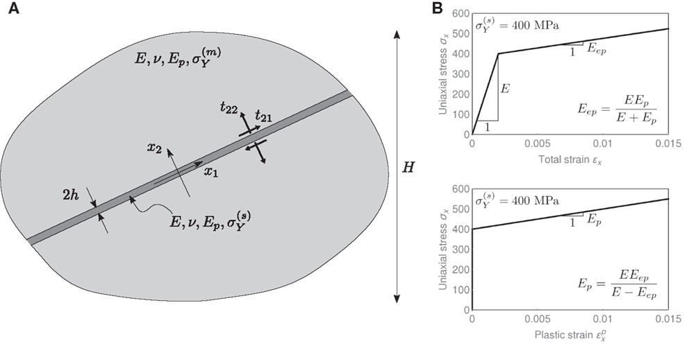
Figure 3. (A) A shear band inside a ductile material modeled as a thin layer of highly compliant material (E_ep/E ≪ 1) embedded in a material block characterized by a dimension H, such that h/H ≪ 1; both materials obey the same von Mises plasticity model represented by the uniaxial stress behavior reported in (B), but having a different yield stress (lower inside than outside the shear band).

At the initial yielding, the material inside the layer [characterized by a low hardening modulus E_ep = EE_p/(E + Ep)] is much more compliant than the material outside (characterized by an elastic isotropic response E).

For h/H ≪ 1, the transmission conditions across the layer imply the continuity of the tractions, t = [t₂₁, t₂₂]^T, which can be expressed in the asymptotic form

$〚t_{21}〛=O\left(h\right),〚t_{22}〛=O\left(h\right),$ (1)

where 〚⋅〛 denotes the jump operator.

The jump in displacements, 〚u〛 = [〚u₁〛, 〚u₂〛]^T, across the layer is related to the tractions at its boundaries through the asymptotic relations (Mishuris et al., 2013; Sonato et al., 2015)

$t_{21}\left(〚u_1〛,〚u_2〛\right)=\frac{E_p\sqrt{3{〚u_1〛}^2+4{〚u_2〛}^2}+6h{\mathrm{\sigma }}_Y^{\left(s\right)}}{\left(3E+2\left(1+\mathrm{\nu }\right)E_p\right)\sqrt{3{〚u_1〛}^2+4{〚u_2〛}^2}}\frac{E〚u_1〛}{2h}+O\left(h\right),$ (2)

$t_{22}\left(〚u_1〛,〚u_2〛\right)=\frac{\left(E+2\left(1-\mathrm{\nu }\right)E_p\right)\sqrt{3{〚u_1〛}^2+4{〚u_2〛}^2}+\mathrm{\hspace{0.17em}8}h\left(1-\mathrm{2\nu }\right){\mathrm{\sigma }}_Y^{\left(s\right)}}{\left(1-\mathrm{2\nu }\right)\left(3E+2\left(1+\mathrm{\nu }\right)E_p\right)\sqrt{3{〚u_1〛}^2+4{〚u_2〛}^2}}\frac{E〚u_2〛}{2h}+O\left(h\right),$ (3)

involving the semi-thickness h of the shear band, which enters the formulation as a constitutive parameter for the zero-thickness interface model and introduces a length scale. Note that, by neglecting the remainder O(h), equations (2) and (3) define non-linear relationships between tractions and jump in displacements.

The time derivative of equations (2) and (3) yields the following asymptotic relation between incremental quantities

$\dot{t}\sim \left[\frac{1}{h}{\mathit{K}}_{-1}+{\mathit{K}}_0\left(〚u_1〛,〚u_2〛\right)\right]〚\dot{\mathit{u}}〛,$ (4)

where the two stiffness matrices K₋₁ and K₀ are given by

${\mathit{K}}_{-1}=\frac{E}{2\left(3E+2\left(1+\mathrm{\nu }\right)E_p\right)}\left[\begin{array}{cc}\hfill E_p\hfill & \hfill 0\hfill \\ \hfill 0\hfill & \hfill \frac{E+2\left(1-\mathrm{\nu }\right)E_p}{1-\mathrm{2\nu }}\hfill \end{array}\right],$ (5)

${\mathit{K}}_0=\frac{12E{\mathrm{\sigma }}_Y^{\left(s\right)}}{\left(3E+2\left(1+\mathrm{\nu }\right)E_p\right){\left(3{〚u_1〛}^2+4{〚u_2〛}^2\right)}^{3/2}}\times \left[\begin{array}{cc}\hfill {〚u_2〛}^2\hfill & \hfill -〚u_1〛〚u_2〛\hfill \\ \hfill -〚u_1〛〚u_2〛\hfill & \hfill {〚u_1〛}^2\hfill \end{array}\right],$ (6)

Assuming now a perfectly plastic behavior, E_p = 0, in the limit h/H → 0 the condition

$〚u_2〛=0$ (7)

is obtained, so that the incremental transmission conditions equation (4) can be approximated to the leading order as

$\dot{\mathit{t}}\sim \frac{1}{h}{\mathit{K}}_{-1}〚\dot{\mathit{u}}〛.$ (8)

Therefore, when the material inside the layer is close to the perfect plasticity condition, the incremental conditions assume the limit value

${\dot{t}}_{21}=0,〚{\dot{u}}_2〛=0,$ (9)

which, together with the incremental version of equation (1)₂, namely,

$〚{\dot{t}}_{22}〛=0,$ (10)

correspond to the incremental boundary conditions proposed in Bigoni and Dal Corso (2008) to define a pre-existing shear band of null thickness.

The limit relations, equations (9) and (10), motivate the use of the imperfect interface approach (Bigoni et al., 1998; Antipov et al., 2001; Mishuris, 2001, 2004; Mishuris and Kuhn, 2001; Mishuris and Ochsner, 2005, 2007) for the modeling of shear band growth in a ductile material. A computational model, in which the shear bands are modeled as interfaces, is presented in the next section.

3. Numerical Simulations

Two-dimensional plane-strain finite element simulations are presented to show the effectiveness of the above-described asymptotic model for a thin and highly compliant layer in modeling a shear band embedded in a ductile material. Specifically, we will show that the model predicts rectilinear propagation of a shear band under simple shear boundary conditions and it allows the investigation of the stress concentration at the shear band tip.

The geometry and material properties of the model are shown in Figure 4, where a rectangular block of edges H and L ≥ H is subject to boundary conditions consistent with a simple shear deformation, so that the lower edge of the square domain is clamped, the vertical displacements are constrained along the vertical edges and along the upper edge, where a constant horizontal displacement u₁ is prescribed. The domain is made of a ductile material and contains a thin (h/H ≪ 1) and highly compliant (E_ep/E ≪ 1) layer of length H/2 and thickness 2h = 0.01 mm, which models a shear band. The material constitutive behavior is described by an elastoplastic model based on linear isotropic elasticity (E = 200000 MPa, v = 0.3) and von Mises plasticity with linear hardening (the plastic modulus is denoted by E_p). The uniaxial yield stress ${\mathrm{\sigma }}_Y^{\left(m\right)}$ for the matrix material is equal to 500 MPa, whereas the layer is characterized by a lower yield stress, namely, ${\mathrm{\sigma }}_Y^{\left(s\right)}=400\mathrm{\hspace{0.17em}MPa}.$

FIGURE 4

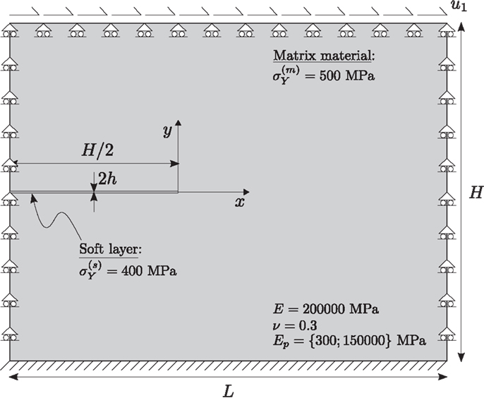
Figure 4. Geometry of the model, material properties, and boundary conditions (which would correspond to a simple shear deformation in the absence of the shear band). The horizontal displacement u₁ is prescribed at the upper edge of the domain.

The layer remains neutral until yielding, but, starting from that stress level, it becomes a material inhomogeneity, being more compliant (because its response is characterized by E_ep) than the matrix (still in the elastic regime and thus characterized by E). The layer can be representative of a pre-existing shear band and can be treated with the zero-thickness interface model, equations (2) and (3). This zero-thickness interface was implemented in the ABAQUS finite element software⁶ through cohesive elements, equipped with the traction-separation laws, equations (2) and (3), by means of the user subroutine UMAT. An interface, embedded into the cohesive elements, is characterized by two dimensions: a geometrical and a constitutive thickness. The latter, 2h, exactly corresponds to the constitutive thickness involved in the model for the interface equations (2) and (3), while the former, denoted by 2h_g, is related to the mesh dimension in a way that the results become independent of this parameter, in the sense that a mesh refinement yields results converging to a well-defined solution.

We consider two situations. In the first, we assume that the plastic modulus is E_p = 150000 MPa (both inside and outside the shear band), so that the material is in a state far from a shear band instability (represented by loss of ellipticity of the tangent constitutive operator, occurring at E_p = 0) when at yield. In the second, we assume that the material is prone to a shear band instability, though still in the elliptic regime, so that E_p (both inside and outside the shear band) is selected to be “sufficiently small”, namely, E_p = 300 MPa. The pre-existing shear band is therefore employed as an imperfection triggering shear strain localization when the material is still inside the region, but close to the boundary, of ellipticity.

3.1. Description of the Numerical Model

With reference to a square block (L = H = 10 mm) containing a pre-existing shear band with constitutive thickness h = 0.005 mm, three different meshes were used, differing in the geometrical thickness of the interface representing the pre-existing shear band (see Figure 5 where the shear band is highlighted with a black line), namely, h_g = {0.05; 0.005; 0.0005} mm corresponding to coarse, fine, and ultra-fine meshes.

FIGURE 5

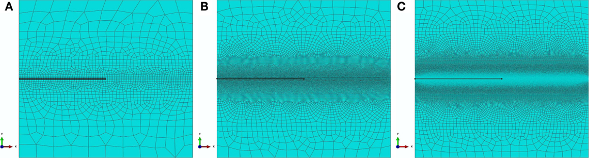
Figure 5. The three meshes used in the analysis to simulate a shear band (highlighted in black) in a square solid block (L = H = 10 mm). The shear band is represented in the three cases as an interface with the same constitutive thickness h = 0.005 mm, but with decreasing geometric thickness h_g; (A) coarse mesh (1918 nodes, 1874 elements, h_g = 0.05 mm); (B) fine mesh (32,079 nodes, 31,973 elements, h_g = 0.005 mm); (C) ultra-fine mesh (1,488,156 nodes, 1,487,866 elements, h_g = 0.0005 mm).

The three meshes were generated automatically using the mesh generator available in ABAQUS. In order to have increasing mesh refinement from the exterior (upper and lower parts) to the interior (central part) of the domain, where the shear band is located, and to ensure the appropriate element shape and size according to the geometrical thickness 2h_g, the domain was partitioned into rectangular subdomains with increasing mesh seeding from the exterior to the interior. Afterwards, the meshes were generated by employing a free meshing technique with quadrilateral elements and the advancing front algorithm.

The interface that models the shear band is discretized using 4-node two-dimensional cohesive elements (COH2D4), while the matrix material is modeled using 4-node bilinear, reduced integration with hourglass control (CPE4R).

It is important to note that the constitutive thickness used for traction-separation response is always equal to the actual size of the shear band h = 0.005 mm, whereas the geometric thickness h_g, defining the height of the cohesive elements, is different for the three different meshes. Consequently, all the three meshes used in the simulations correspond to the same problem in terms of both material properties and geometrical dimensions (although the geometric size of the interface is different), so that the results have to be, and indeed will be shown to be, mesh independent⁷.

3.2. Numerical Results

Results (obtained using the fine mesh, Figure 5B) in terms of the shear stress component σ₁₂ at different stages of a deformation process for the boundary value problem sketched in Figure 4 are reported in Figures 6 and 7.

FIGURE 6

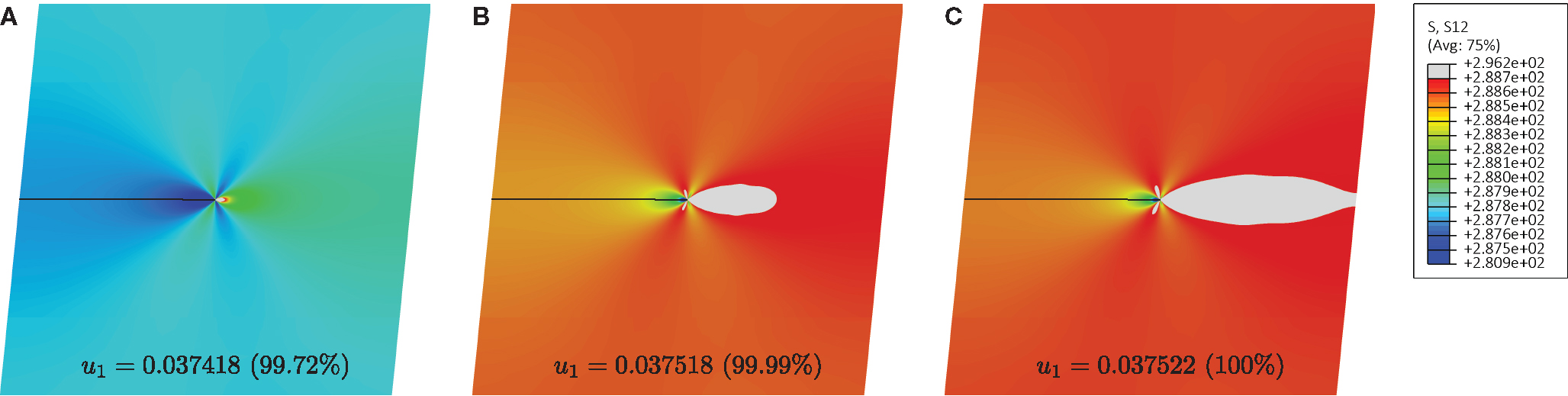
Figure 6. Contour plots of the shear stress σ₁₂ for the case of material far from shear band instability (E_p = 150000 MPa). The gray region corresponds to the material at yielding ${\mathrm{\sigma }}_{12}\ge 500/\sqrt{3}\hspace{0.17em}=\mathrm{\hspace{0.17em}288}.68\mathrm{\hspace{0.17em}MPa}\mathrm{.}$ Three different stages of deformation are shown, corresponding to a prescribed displacement at the upper edge of the square domain u₁ = 0.037418 mm (A), u₁ = 0.037518 mm (B), u₁ = 0.037522 mm (C). The displacements in the figures are amplified by a deformation scale factor of 25 and the percentages refer to the final displacement.

FIGURE 7

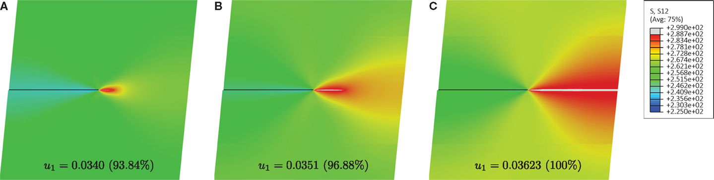
Figure 7. Contour plots of the shear stress σ₁₂ for the case of material close to shear band instability (E_p = 300 MPa). The gray region corresponds to the material at yielding ${\mathrm{\sigma }}_{12}\ge 500/\sqrt{3}.$ Three different stages of deformation are shown, corresponding to a prescribed displacement at the upper edge of the square domain u₁ = 0.0340 mm (A), u₁ = 0.0351 mm (B), u₁ = 0.03623 mm (C). The displacements in the figures are amplified by a deformation scale factor of 27.

In particular, Figure 6 refers to a matrix with high plastic modulus, E_p = 150000 MPa, so that the material is far from the shear band formation threshold. The upper limit of the contour levels was set to the value ${\mathrm{\sigma }}_{12}=500/\sqrt{3}\simeq 288.68\mathrm{\hspace{0.17em}MPa},$ corresponding to the yielding stress of the matrix material. As a result, the gray zone in the figure represents the material at yielding, whereas the material outside the gray zone is still in the elastic regime. Three stages of deformation are shown, corresponding to: the initial yielding of the matrix material (left), the yielding zone occupying approximately one-half of the space between the shear band tip and the right edge of the domain (center), and the yielding completely linking the tip of the shear band to the boundary (right). Note that the shear band, playing the role of a material imperfection, produces a stress concentration at its tip. However, the region of high stress level rapidly grows and diffuses in the whole domain. At the final stage, shown in Figure 6C, almost all the matrix material is close to yielding.

Figure 7 refers to a matrix with low plastic modulus, E_p = 300 MPa, so that the material is close (but still in the elliptic regime) to the shear band formation threshold (E_p = 0). Three stages of deformation are shown, from the condition of initial yielding of the matrix material near the shear band tip (left), to an intermediate condition (center), and finally to the complete yielding of a narrow zone connecting the shear band tip to the right boundary (right). In this case, where the material is prone to shear band localization, the zone of high stress level departs from the shear band tip and propagates toward the right. This propagation occurs in a highly concentrated narrow layer, rectilinear, and parallel to the pre-existing shear band. At the final stage of deformation, shown in Figure 7C, the layer of localized shear has reached the boundary of the block.

Results in terms of the shear strain component γ₁₂, for both cases of material far from, and close to shear band instability are reported in Figures 8 and 9, respectively. In particular, Figure 8 shows contour plots of the shear deformation γ₁₂ for the case of a material far from the shear band instability (E_p = 150000 MPa) at the same three stages of deformation as those reported in Figure 6. Although the tip of the shear band acts as a strain raiser, the contour plots show that the level of shear deformation is high and remains diffused in the whole domain.

FIGURE 8

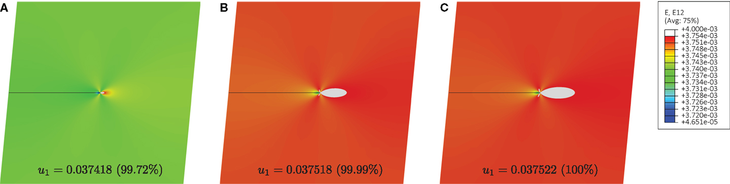
Figure 8. Contour plots of the shear deformation γ₁₂ for the case of material far from shear band instability (E_p = 150000 MPa). Three different stages of deformation are shown, corresponding to a prescribed displacement at the upper edge of the square domain u₁ = 0.037418 mm (A), u₁ = 0.037518 mm (B), u₁ = 0.037522 mm (C). The displacements in the figures are amplified by a deformation scale factor of 25.

FIGURE 9

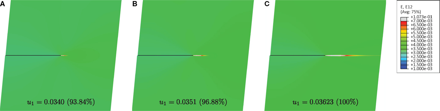
Figure 9. Contour plots of the shear deformation γ₁₂ for the case of material close to shear band instability (E_p = 300 MPa). Three different stages of deformation are shown, corresponding to a prescribed displacement at the upper edge of the square domain u₁ = 0.0340 mm (A), u₁ = 0.0351 mm (B), u₁ = 0.03623 mm (C). The displacements in the figures are amplified by a deformation scale factor of 27.

Figure 9 shows contour plots of the shear deformation γ₁₂ for the case of a material close to the shear band instability (E_p = 300 MPa), at the same three stages of deformation as those reported in Figure 7. It is noted that the shear deformation is localized along a rectilinear path ahead of the shear band tip, confirming results that will be reported later with the perturbation approach (Section 4).

The shear deformation γ₁₂ and the shear stress σ₁₂ along the x-axis containing the pre-existing shear band for the case of a material close to strain localization, E_p = 300 MPa, are shown in Figure 10, upper and lower parts, respectively. Results are reported for the three meshes, coarse, fine and ultra-fine (Figure 5) and at the same three stages of deformation as those shown in Figures 7 and 9. The results appear to be mesh independent, meaning that the solution converges as the mesh is more and more refined.

FIGURE 10

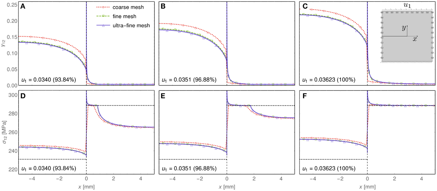
Figure 10. Shear deformation γ₁₂ (A–C) and shear stress σ₁₂ (D–F) along the x-axis containing the pre-existing shear band for the case of a material close to a shear band instability E_p = 300 MPa. The black dotted line, in the bottom part of the figure, indicates the yield stress level, lower inside the pre-existing shear band than that in the outer domain. Three different stages of deformation are shown, corresponding to a prescribed displacement at the upper edge of the square domain u₁ = 0.0340 mm (left), u₁ = 0.0351 mm (center), u₁ = 0.03623 mm (right).

The deformation process reported in Figures 7, 9, and 10 can be described as follows. After an initial homogeneous elastic deformation (not shown in the figure), in which the shear band remains neutral (since it shares the same elastic properties with the matrix material), the stress level reaches ${\mathrm{\sigma }}_{12}=400/\sqrt{3}\simeq 230.9\mathrm{\hspace{0.17em}MPa},$ corresponding to the yielding of the material inside the shear band. Starting from this point, the pre-existing shear band is activated, which is confirmed by a high shear deformation γ₁₂ and a stress level above the yield stress inside the layer, −5 mm < x < 0 (left part of Figure 10). The activated shear band induces a strain localization and a stress concentration at its tip, thus generating a zone of material at yield, which propagates to the right (central part of Figure 10) until collapse (right part of Figure 10).

In order to appreciate the strain and stress concentration at the shear band tip, a magnification of the results shown in Figure 10 in the region −0.2 mm < x < 0.2 mm is presented in Figure 11. Due to the strong localization produced by the shear band, only the ultra-fine mesh is able to capture accurately the strain and stress raising (blue solid curve), whereas the coarse and fine meshes smooth over the strain and stress levels (red dotted and green dashed curves, respectively). The necessity of an ultra-fine mesh to capture details of the stress/strain fields is well-known in computational fracture mechanics, where special elements (quarter-point or extended elements) have been introduced to avoid the use of these ultra-fine meshes at corner points.

FIGURE 11

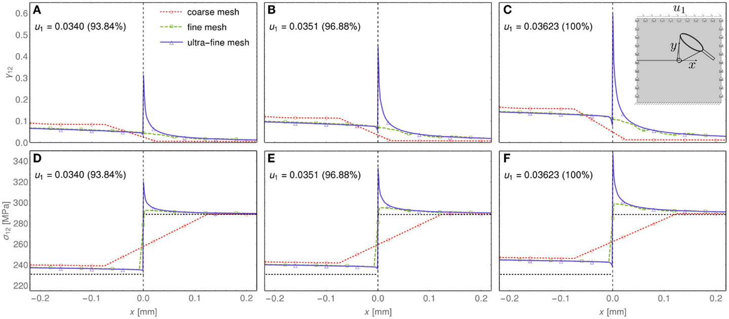
Figure 11. Shear and stress concentration at the shear band tip. Shear deformation γ₁₂ (A–C) and shear stress σ₁₂ (D–F) along the x-axis containing the pre-existing shear band for the case of a material close to a shear band instability E_p = 300 MPa. Three different stages of deformation are shown, corresponding to a prescribed displacement at the upper edge of the square domain u₁ = 0.0340 mm (left), u₁ = 0.0351 mm (center), u₁ = 0.03623 mm (right).

For the purpose of a comparison with an independent and fully numerical representation of the shear band, a finite element simulation was also performed, using standard continuum elements (CPE4R) instead of cohesive elements (COH2D4) inside the layer. This simulation is important to assess the validity of the asymptotic model of the layer presented in Section 2. In this simulation, reported in Figure 12, the layer representing the shear band is a “true” layer of a given and finite thickness, thus influencing the results (while these are independent of the geometrical thickness 2h_g of the cohesive elements, when the constitutive thickness 2h is the same). Therefore, only the fine mesh, shown in Figure 5B, was used, as it corresponds to the correct size of the shear band. The coarse mesh (Figure 5A) and the ultra-fine mesh (Figure 5C) would obviously produce different results, corresponding, respectively, to a thicker or thinner layer. Results pertaining to the asymptotic model, implemented into the traction-separation law for the cohesive elements COH2D4, are also reported in the figure (red solid curve) and are spot-on with the results obtained with a fully numerical solution employing standard continuum elements CPE4R (blue dashed curve).

FIGURE 12

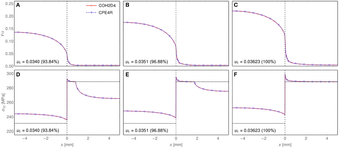
Figure 12. Results of simulations performed with different idealizations for the shear band: zero-thickness model (discretized with cohesive elements, COH2D4) versus a true layer description (discretized with CPE4R elements). Shear deformation γ₁₂ (A–C) and shear stress σ₁₂ (D–F) along the horizontal line y = 0 containing the pre-existing shear band for the case of a material close to a shear band instability E_p = 300 MPa. Three different stages of deformation are shown, corresponding to a prescribed displacement at the upper edge of the square domain u₁ = 0.0340 mm (left), u₁ = 0.0351 mm (center), u₁ = 0.03623 mm (right).

A mesh of the same size as that previously called “fine” was used to perform a simulation of a rectangular block (H = 10 mm, L = 4 H = 40 mm) made up of a material close to shear band instability (E_p = 300 MPa) and containing a shear band (of length H/2 = 5 mm and constitutive thickness 2h = 0.01 mm). Results are presented in Figure 13. In parts (Figures 13A,B) (the latter is a detail of part Figure 13A) of this figure the overall response curve is shown of the block in terms of average shear stress ${\overline{\sigma }}_{12}=T/L$ (T denotes the total shear reaction force at the upper edge of the block) and average shear strain ${\overline{\gamma }}_{12}=u_1/H.$ In part (Figure 13C) of the figure contour plots of the shear deformation γ₁₂ are reported at different stages of deformation. It is clear that the deformation is highly focused along a rectilinear path emanating from the shear band tip, thus demonstrating the tendency of the shear band toward rectilinear propagation under shear loading.

FIGURE 13

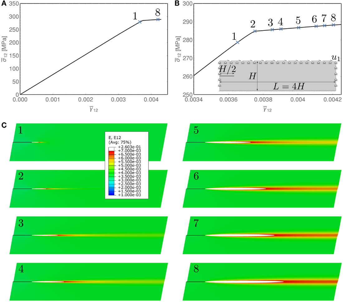
Figure 13. Results for a rectangular domain (L = 40 mm, H = 10 mm) of material close to shear band instability (E_p = 300 MPa) and containing a pre-existing shear band (of length H/2 = 5 mm and constitutive thickness 2h = 0.01 mm). (A) Overall response curve of the block in terms of average shear stress ${\overline{\sigma }}_{12}=T/L,$ where T is the total shear reaction force at the upper edge of the block, and average shear strain ${\overline{\gamma }}_{12}=u_1/H.$(B) Magnification of the overall response curve ${\overline{\sigma }}_{12}-{\overline{\gamma }}_{12}$ around the stress level corresponding to the yielding of the shear band. (C) Contour plots of the shear deformation γ₁₂ at different stages of deformation, corresponding to the points along the overall response curve shown in (B) of the figure. The deformation is highly focused along a rectilinear path emanating from the shear band tip. The displacements in the figures are amplified by a deformation scale factor of 50.

Finally, the incremental shear strain (divided by the mean incremental shear strain) has been reported along the x-axis in Figure 14, at the two stages of deformation considered in Figure 10 and referred there as (Figures 10A,C). These results, which have been obtained with the fine mesh, show that a strong incremental strain concentration develops at the shear band tip and becomes qualitatively similar to the square-root singularity found in the perturbative approach.

FIGURE 14

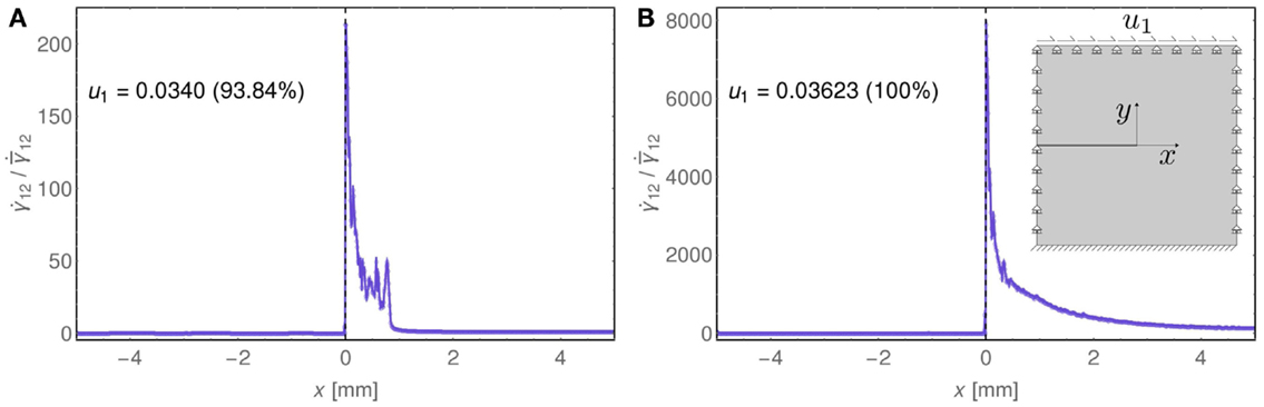
Figure 14. The incremental shear strain ${\dot{\gamma }}_{12}$ (divided by the mean incremental shear strain ${\dot{\overline{\gamma }}}_{12}$) along the x-axis at the two stages of deformation, (A) u₁ = 0. 0340 mm and (B) u₁ = 0. 03623 mm, reported in Figure 10 and labeled there as (Figures 10A,C). It is clear that a strong strain concentration develops at the tip of the shear band, which becomes similar to the square-root singularity that is found with the perturbative approach (Section 4 and Figure 16).

4. The Perturbative Versus the Imperfection Approach

With the perturbative approach, a perturbing agent acts at a certain stage of uniform strain of an infinite body, while the material is subject to a uniform prestress. Here, the perturbing agent is a pre-existing shear band, modeled as a planar slip surface, emerging at a certain stage of a deformation path (Bigoni and Dal Corso, 2008), in contrast with the imperfection approach in which the imperfection is present from the beginning of the loading.

With reference to a x₁ − x₂ coordinate system (inclined at 45° with respect to the principal prestress axes x_I – x_II), where the incremental stress ${ṫ}_{\mathit{ij}}$ and incremental strain ${\dot{\epsilon }}_{\mathit{ij}}$ are defined (i, j = 1, 2), the incremental orthotropic response under plane-strain conditions $\left({\dot{\epsilon }}_{i3}=0\right)$ for incompressible materials $\left({\dot{\epsilon }}_{11}+{\dot{\epsilon }}_{22}=0\right)$ can be expressed through the following constitutive equations (Bigoni, 2012)⁸.

${ṫ}_{11}=\mathrm{2\mu }{\dot{\epsilon }}_{11}+ṗ,{ṫ}_{22}=-\mathrm{2\mu }{\dot{\epsilon }}_{11}+ṗ,{ṫ}_{12}={\mu }_{\ast }{\dot{\gamma }}_{12},$ (11)

where $ṗ$ is the incremental in-plane mean stress, while μ and μ_∗ describe the incremental shear stiffness, respectively, parallel and inclined at 45° with respect to prestress axes.

The assumption of a specific constitutive model leads to the definition of the incremental stiffness moduli μ and μ_*. With reference to the J₂-deformation theory of plasticity (Bigoni and Dal Corso, 2008), particularly suited to model the plastic branch of the constitutive response of ductile metals, the in-plane deviatoric stress can be written as

$t_I-t_{\mathit{II}}=k{\mathrm{\epsilon }}_I|{\mathrm{\epsilon }}_I{|}^{\left(N-1\right)}.$ (12)

In equation (12), k represents a stiffness coefficient and N ∈ (0, 1] is the strain hardening exponent, describing perfect plasticity (null hardening) in the limit N → 0 and linear elasticity in the limit N → 1. For the J₂-deformation theory, the relation between the two incremental shear stiffness moduli can be obtained as

${\mu }_{\ast }=N\mu ,$ (13)

so that a very compliant response under shear (μ_∗ ≪ μ) is described in the limit of perfect plasticity N → 0.

The perturbative approach (Bigoni and Dal Corso, 2008) can now be exploited to investigate the growth of a shear band within a solid. To this purpose, an incremental boundary value problem is formulated for an infinite solid, containing a zero-thickness pre-existing shear band of finite length 2l parallel to the x₁ axis (see Figure 15) and loaded at infinity through a uniform shear deformation ${\dot{\gamma }}_{12}^{\infty }.$

FIGURE 15

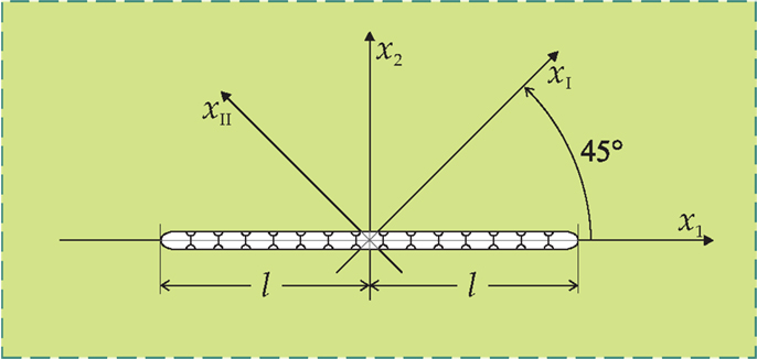
Figure 15. A perturbative approach to shear band growth: a pre-existing shear band, modeled as a planar slip surface, acts at a certain stage of uniform deformation of an infinite body obeying the J₂-deformation theory of plasticity.

The incremental boundary conditions introduced by the presence of a pre-existing shear band can be described by the following equations:

${ṫ}_{21}\left(x_1,0^{\pm }\right)=0,〚{ṫ}_{22}\left(x_1,0\right)〛=0,〚{\dot{u}}_2\left(x_1,0\right)〛=0,\forall \left|x_1\right|<l.$ (14)

A stream function ψ(x₁, x₂) is now introduced, automatically satisfying the incompressibility condition and defining the incremental displacements ${\dot{u}}_j$ as ${\dot{u}}_1={\mathrm{\psi }}_{,2},$ and ${\dot{u}}_2=-{\mathrm{\psi }}_{,1}.$ The incremental boundary value problem is therefore solved as the sum of ψ°(x₁, x₂), solution of the incremental homogeneous problem, and ψ^p(x₁, x₂), solution of the incremental perturbed problem.

The incremental solution is reported in Figure 16 for a low hardening exponent, N = 0.01, as a contour plot (left) and as a graph (along the x₁-axis, right) of the incremental shear deformation ${\dot{\gamma }}_{12}$ (divided by the applied remote shear ${\dot{\gamma }}_{12}^{\infty }$). Note that, similarly to the crack tip fields in fracture mechanics, the incremental stress and deformation display square-root singularities at the tips of the pre-existing shear band. Evaluation of the solution obtained from the perturbative approach analytically confirms the conclusions drawn from the imperfection approach (see the numerical simulations reported in Figures 9 and 13), in particular:

• It can be noted from Figure 16 (left) that the incremental deformation is highly focused along the x₁ direction, confirming that the shear band grows rectilinearly;

• The blow-up of the incremental deformation observed in the numerical simulations near the shear band tip (Figure 14) is substantiated by the theoretical square-root singularity found in the incremental solution (Figure 16, right).

We finally remark that, although the tendency toward rectilinear propagation of a shear band has been substantiated through the use of a von Mises plastic material, substantial changes are not expected when a different yield criterion (for instance, pressure-sensitive as Drucker–Prager) is employed.

FIGURE 16

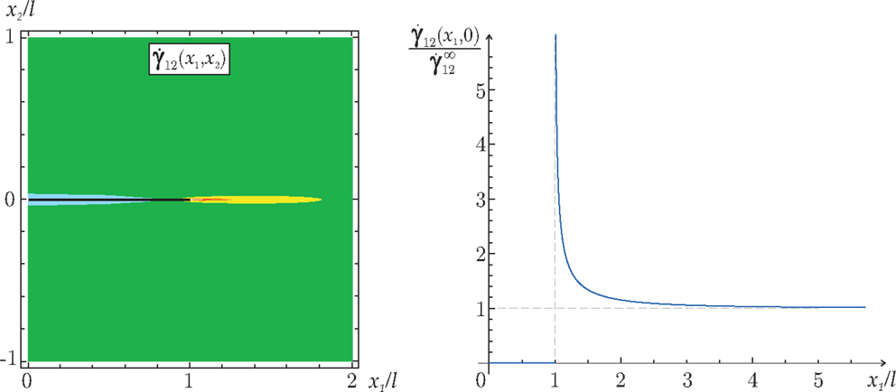
Figure 16. Incremental shear strain near a shear band obtained through the perturbative approach: level sets (left) and behavior along the x₁-axis (right).

5. Conclusion

Two models of shear band have been described, one in which the shear band is an imperfection embedded in a material and another in which the shear band is a perturbation, which emerges during a homogeneous deformation of an infinite material. These two models explain how shear bands tend toward a rectilinear propagation under continuous shear loading, a feature not observed for fracture trajectories in brittle materials. This result can be stated in different words pointing out that, while crack propagation occurs following a maximum tensile stress criterion, a shear band grows according to a maximum Mises stress, a behavior representing a basic micromechanism of failure for ductile materials. The developed models show also a strong stress concentration at the shear band tip, which strongly concur to shear band growth.

Conflict of Interest Statement

The authors declare that the research was conducted in the absence of any commercial or financial relationships that could be construed as a potential conflict of interest.

Acknowledgments

DB, NB, and FDC gratefully acknowledge financial support from the ERC Advanced Grant “Instabilities and non-local multiscale modeling of materials” FP7-PEOPLE-IDEAS-ERC-2013-AdG (2014-2019). AP thanks financial support from the FP7-PEOPLE-2013-CIG grant PCIG13-GA-2013-618375-MeMic.

Footnotes

1. ^For granular materials, there are cases in which unloading occurs inside the shear band, as shown by Gajo et al. (2004).
2. ^The proposed explanation for the crack patterns shown in Figure 2 relies on the fact that the fracture network has formed during the plastic evolution of a ductile homogeneously deformed material. Other explanations may be related to bonding of an external layer to a rigid substrate (Peron et al., 2013), or to surface instability (Destrade and Merodio, 2011; Boulogne et al., 2015), or to instabilities occurring during shear (Destrade et al., 2008; Ciarletta et al., 2013).
3. ^Special problems of shear band propagation in geological materials have been addressed by Puzrin and Germanovich (2005) and Rice (1973).
4. ^A different approach to investigate shear band evolution is based on the exploitation of phase-field models (Zheng and Li, 2009), which has been often used for brittle fracture propagation (Miehe et al., 2010).
5. ^To highlight the differences and the analogies between the two approaches, the incremental strain field induced by the emergence of a shear band of finite length (modeled as a sliding surface) is determined for a J₂-deformation theory material and compared with finite element simulations in which the shear band is modeled as a zero-thickness layer of compliant material.
6. ^ABAQUS Standard Ver. 6.13 has been used, available on the AMD Opteron cluster Stimulus at UniTN.
7. ^Note that, in the case of null hardening, mesh dependency may occur in the simulation of shear banding nucleation and propagation (Needleman, 1988; Loret and Prevost, 1991, 1993). This numerical issue can be avoided by improving classical inelastic models through the introduction of characteristic length-scales (Lapovok et al., 2009; Dal Corso and Willis, 2011).
8. ^Note that the notation used here differs from that adopted in Bigoni and Dal Corso (2008), where the principal axes are denoted by x₁ and x₂ and the system inclined at 45° is denoted by ${\widehat{x}}_1$ and ${\widehat{x}}_2$.

References

Abeyaratne, R., and Triantafyllidis, N. (1981). On the emergence of shear bands in plane strain. Int. J. Solids Struct. 17, 1113–1134. doi: 10.1016/0020-7683(81)90092-5

Pubmed Abstract | Pubmed Full Text | CrossRef Full Text | Google Scholar

Antipov, Y. A., Avila-Pozos, O., Kolaczkowski, S. T., and Movchan, A. B. (2001). Mathematical model of delamination cracks on imperfect interfaces. Int. J. Solids Struct. 38, 6665–6697. doi:10.1016/S0020-7683(01)00027-0

CrossRef Full Text | Google Scholar

Argani, L., Bigoni, D., Capuani, D., and Movchan, N. V. (2014). Cones of localized shear strain in incompressible elasticity with prestress: Green’s function and integral representations. Proc. Math. Phys. Eng. Sci. 470, 20140423. doi:10.1098/rspa.2014.0423

Pubmed Abstract | Pubmed Full Text | CrossRef Full Text | Google Scholar

Argani, L., Bigoni, D., and Mishuris, G. (2013). Dislocations and inclusions in prestressed metals. Proc. R. Soc. A 469, 20120752. doi:10.1098/rspa.2012.0752

CrossRef Full Text | Google Scholar

Bacigalupo, A., and Gambarotta, L. (2013). A multi-scale strain-localization analysis of a layered strip with debonding interfaces. Int. J. Solids Struct. 50, 2061–2077. doi:10.1016/j.ijsolstr.2013.03.006

CrossRef Full Text | Google Scholar

Bigoni, D. (2012). Nonlinear Solid Mechanics Bifurcation Theory and Material Instability. New York: Cambridge University Press.

Google Scholar

Bigoni, D., and Capuani, D. (2002). Green’s function for incremental nonlinear elasticity: shear bands and boundary integral formulation. J. Mech. Phys. Solids 50, 471–500. doi:10.1016/S0022-5096(01)00090-4

Pubmed Abstract | Pubmed Full Text | CrossRef Full Text | Google Scholar

Bigoni, D., and Capuani, D. (2005). Time-harmonic Green’s function and boundary integral formulation for incremental nonlinear elasticity: dynamics of wave patterns and shear bands. J. Mech. Phys. Solids 53, 1163–1187. doi:10.1016/j.jmps.2004.11.007

CrossRef Full Text | Google Scholar

Bigoni, D., and Dal Corso, F. (2008). The unrestrainable growth of a shear band in a prestressed material. Proc. R. Soc. A 464, 2365–2390. doi:10.1098/rspa.2008.0029

CrossRef Full Text | Google Scholar

Bigoni, D., Dal Corso, F., and Gei, M. (2008). The stress concentration near a rigid line inclusion in a prestressed, elastic material. Part II. Implications on shear band nucleation, growth and energy release rate. J. Mech. Phys. Solids 56, 839–857. doi:10.1016/j.jmps.2007.07.003

CrossRef Full Text | Google Scholar

Bigoni, D., Serkov, S. K., Movchan, A. B., and Valentini, M. (1998). Asymptotic models of dilute composites with imperfectly bonded inclusions. Int. J. Solids Struct. 35, 3239–3258. doi:10.1016/S0020-7683(97)00366-1

CrossRef Full Text | Google Scholar

Boulogne, F., Giorgiutti-Dauphine, F., and Pauchard, L. (2015). Surface patterns in drying films of silica colloidal dispersions. Soft Matter 11, 102. doi:10.1039/c4sm02106a

Pubmed Abstract | Pubmed Full Text | CrossRef Full Text | Google Scholar

Ciarletta, P., Destrade, M., and Gower, A. L. (2013). Shear instability in skin tissue. Q. J. Mech. Appl. Math. 66, 273–288. doi:10.1097/TA.0b013e3182092e66

Pubmed Abstract | Pubmed Full Text | CrossRef Full Text | Google Scholar

Dal Corso, F., and Bigoni, D. (2009). The interactions between shear bands and rigid lamellar inclusions in a ductile metal matrix. Proc. R. Soc. A 465, 143–163. doi:10.1098/rspa.2008.0242

CrossRef Full Text | Google Scholar

Dal Corso, F., and Bigoni, D. (2010). Growth of slip surfaces and line inclusions along shear bands in a softening material. Int. J. Fract. 166, 225–237. doi:10.1007/s10704-010-9534-1

CrossRef Full Text | Google Scholar

Dal Corso, F., Bigoni, D., and Gei, M. (2008). The stress concentration near a rigid line inclusion in a prestressed, elastic material. Part I. Full field solution and asymptotics. J. Mech. Phys. Solids 56, 815–838. doi:10.1016/j.jmps.2007.07.002

CrossRef Full Text | Google Scholar

Dal Corso, F., and Willis, J. R. (2011). Stability of strain-gradient plastic materials. J. Mech. Phys. Solids 59, 1251–1267. doi:10.1016/j.jmps.2011.01.014

CrossRef Full Text | Google Scholar

Danas, K., and Ponte Castaneda, P. (2012). Influence of the Lode parameter and the stress triaxiality on the failure of elasto-plastic porous materials. Int. J. Solids Struct. 49, 1325–1342. doi:10.1016/j.ijsolstr.2012.02.006

CrossRef Full Text | Google Scholar

Destrade, M., Gilchrist, M., Prikazchikov, D., and Saccomandi, G. (2008). Surface instability of sheared soft tissues. J. Biomech. Eng. 130, 061007. doi:10.1115/1.2979869

Pubmed Abstract | Pubmed Full Text | CrossRef Full Text | Google Scholar

Destrade, M., and Merodio, J. (2011). Compression instabilities of tissues with localized strain softening. Int. J. Appl. Mech. 3, 69–83. doi:10.1142/S1758825111000877

CrossRef Full Text | Google Scholar

Gajo, A., Bigoni, D., and Muir Wood, D. (2004). Multiple shear band development and related instabilities in granular materials. J. Mech. Phys. Solids 52, 2683–2724. doi:10.1016/j.jmps.2004.05.010

CrossRef Full Text | Google Scholar

Hill, R. (1962). Acceleration waves in solids. J. Mech. Phys. Solids 10, 1–16. doi:10.1016/0022-5096(62)90024-8

CrossRef Full Text | Google Scholar

Hutchinson, J. W., and Tvergaard, V. (1981). Shear band formation in plane strain. Int. J. Solids Struct. 17, 451–470. doi:10.1111/j.1365-2818.2009.03250.x

Pubmed Abstract | Pubmed Full Text | CrossRef Full Text | Google Scholar

Kirby, S. H. (1985). Rock mechanics observations pertinent to the rheology of the continental lithosphere and the localization of strain along shear zones. Tectonophysics 119, 1–27. doi:10.1016/0040-1951(85)90030-7

CrossRef Full Text | Google Scholar

Lapovok, R., Toth, L. S., Molinari, A., and Estrina, Y. (2009). Strain localisation patterns under equal-channel angular pressing. J. Mech. Phys. Solids 57, 122–136. doi:10.1016/j.jmps.2008.09.012

CrossRef Full Text | Google Scholar

Loret, B., and Prevost, J. H. (1991). On the existence of solutions in layered elasto-(visco-)plastic solids with negative hardening. Eur. J. Mech. A Solids 10, 575–586.

Google Scholar

Loret, B., and Prevost, J. H. (1993). On the occurrence of unloading in 1D elasto- (visco-)plastic structures with softening. Eur. J. Mech. Solids 12, 757–772.

Google Scholar

Mandel, J. (1962). Ondes plastiques dans un milieu indéfini à trois dimensions. J. Mécanique 1, 3–30.

Google Scholar

Miehe, C., Hofacker, M., and Welschinger, F. (2010). A phase field model for rate-independent crack propagation: robust algorithmic implementation based on operator splits. Comput. Methods Appl. Mech. Eng. 199, 2765–2778. doi:10.1016/j.cma.2010.04.011

CrossRef Full Text | Google Scholar

Mishuris, G. (2001). Interface crack and nonideal interface concept (Mode III). Int. J. Fract. 107, 279–296. doi:10.1023/A:1007664911208

CrossRef Full Text | Google Scholar

Mishuris, G. (2004). Imperfect transmission conditions for a thin weakly compressible interface. 2D problems. Arch. Mech. 56, 103–115.

Google Scholar

Mishuris, G., and Kuhn, G. (2001). Asymptotic behaviour of the elastic solution near the tip of a crack situated at a nonideal interface. Z. Angew. Math. Mech. 81, 811–826. doi:10.1002/1521-4001(200112)81:12<811::AID-ZAMM811>3.0.CO;2-I

CrossRef Full Text | Google Scholar

Mishuris, G., Miszuris, W., Ochsner, A. and Piccolroaz, A. (2013). “Transmission conditions for thin elasto-plastic pressure-dependent interphases,” in Plasticity of Pressure-Sensitive Materials, eds H. Altenbach and A. Ochsner (Berlin: Springer-Verlag), 205–251.

Google Scholar

Mishuris, G., and Ochsner, A. (2005). Transmission conditions for a soft elasto-plastic interphase between two elastic materials. Plane Strain State. Arch. Mech. 57, 157–169.

Google Scholar

Mishuris, G., and Ochsner, A. (2007). 2D modelling of a thin elasto-plastic interphase between two different materials: plane strain case. Compos. Struct. 80, 361–372. doi:10.1016/j.compstruct.2006.05.017

CrossRef Full Text | Google Scholar

Nadai, A. (1950). Theory of Flow and Fracture of Solids. New York, NY: McGraw-Hill.

Google Scholar

Needleman, A. (1988). Material rate dependence and mesh sensitivity in localization problems. Comput. Methods Appl. Mech. Eng. 67, 69–75. doi:10.1016/0045-7825(88)90069-2

CrossRef Full Text | Google Scholar

Needleman, A., and Tvergaard, V. (1983). “Finite element analysis of localization in plasticity”, in Finite Elements: Special Problems in Solid Mechanics, Vol. V, eds J. T. Oden and G. F. Carey (Englewood Cliffs: Prentice-Hall), 94–157.

Google Scholar

Peron, H., Laloui, L., Hu, L. B., and Hueckel, T. (2013). Formation of drying crack patterns in soils: a deterministic approach. Acta Geotech. 8, 215–221. doi:10.1007/s11440-012-0184-5

CrossRef Full Text | Google Scholar

Petryk, H. (1997). Plastic instability: criteria and computational approaches. Arch. Comput. Meth. Eng. 4, 111–151. doi:10.1007/BF03020127

CrossRef Full Text | Google Scholar

Piccolroaz, A., Bigoni, D., and Willis, J. R. (2006). A dynamical interpretation of flutter instability in a continuous medium. J. Mech. Phys. Solids 54, 2391–2417. doi:10.1016/j.jmps.2006.05.005

CrossRef Full Text | Google Scholar

Prager, W. (1954). “Discontinuous fields of plastic stress and flow,” in 2nd Nat. Congr. Appl. Mech (Ann Arbor, MI: ASME), 21–32.

Google Scholar

Puzrin, A. M., and Germanovich, L. N. (2005). The growth of shear bands in the catastrophic failure of soils. Proc. R. Soc. A 461, 1199–1228. doi:10.1098/rspa.2004.1378

CrossRef Full Text | Google Scholar

Rice, J. R. (1973). “The initiation and growth of shear bands,” in Plasticity and Soil Mechanics, ed. A. C. Palmer (Cambridge: Cambridge University Engineering Department), 263.

Google Scholar

Rice, J. R. (1977). “The localization of plastic deformation,” in Theoretical and Applied Mechanics, ed. W. T. Koiter (Amsterdam: North-Holland Publishing Co.), 207.

Google Scholar

Sonato, M., Piccolroaz, A., Miszuris, W., and Mishuris, G. (2015). General transmission conditions for thin elasto-plastic pressure-dependent interphase between dissimilar materials. Int. J. Solids Struct. doi:10.1016/j.ijsolstr.2015.03.009

CrossRef Full Text | Google Scholar

Thomas, T. Y. (1961). Plastic Flows and Fracture of Solids. New York, NY: Academic Press.

Google Scholar

Tvergaard, V. (2014). Bifurcation into a localized mode from non-uniform periodic deformations around a periodic pattern of voids. J. Mech. Phys. Solids 69, 112–122. doi:10.1016/j.jmps.2014.05.002

CrossRef Full Text | Google Scholar

Yang, B., Morrison, M. L., Liaw, P. K., Buchanan, R. A., Wang, G., Liu, C. T., et al. (2005). Dynamic evolution of nanoscale shear bands in a bulk-metallic glass. Appl. Phys. Lett. 86, 141904. doi:10.1063/1.1891302

CrossRef Full Text | Google Scholar

Zheng, G. P., and Li, M. (2009). Mesoscopic theory of shear banding and crack propagation in metallic glasses. Phys. Rev. B 80, 104201. doi:10.1103/PhysRevB.80.104201

CrossRef Full Text | Google Scholar