Identification of Grout Sleeve Joint Defect in Prefabricated Structures Using Deep Learning

Introduction

In recent years, prefabricated structures have been widely used in construction, and grout sleeves are the most widely used connection type in these structures. Usually, the special grout used in these connections has good fluidity, early and high strength, and micro-expansion. However, most of these sleeves have complicated internal structures and complicated construction procedures, and this often leads to joint defects during the construction process. The underfilling of sleeve grouting is one of the typical defects that are seen in these connections. Such defects will seriously affect the mechanical properties of the joints and eventually affect the bearing capacity and seismic performance of the overall structure (Zhu et al., 2019). Conveniently and effectively detecting the fullness of sleeve grouting has always been a difficult problem in prefabricated concrete buildings. The ultrasonic wave method (Feng et al., 2020), the impact-echo method (Chou, 2019), the X-ray CT method (Zelelew et al., 2013; Gao et al., 2017), the damped vibration method (Zhu et al., 2018), the X-ray method (du Plessis and Boshoff, 2019), and the embedded wire-drawing method (Gao et al., 2019) are relatively mature detection technologies, but they are expensive and labor intensive, which means they are not conducive to the full detection of sleeve grouting. Because such defects are typically local, traditional global-based non-destructive dynamic testing methods also face great challenges when used with complex structures, because these technologies are unable to obtain effective local feature information from global dynamical data (Yoon et al., 2010). Moreover, with the increasing complexity of these connections, the influences of the different parts will increase, which will lead to these methods being unable to effectively extract feature information.

As a subset of machine learning in artificial intelligence (AI), deep learning involves networks that are capable of learning without supervision from original data. Deep learning technology has the potential to provide a new identification method in a case such as this because it can autonomously learn highly abstract features from original data.

Deep learning has enabled many practical applications of machine learning, and by extension the overall field of AI. An increasing number of researchers have tried to apply deep learning to identification problems in the field of civil engineering. LeCun et al. (1989) developed the first deep convolutional neural network (DCNN) to realize handwritten postcode identification (LeNet-5), using back propagation (BP), a supervised training algorithm. Cha et al. (2017) proposed a crack detection method for concrete structures based on a convolutional neural network (CNN) that used crack photographs taken under different conditions (such as different photo sizes, light sources, and shadows) for testing. Dorafshan et al. (2018) compared the performance of commonly used edge detectors and DCNNs in crack detection in concrete structures and proposed a method combining a DCNN and edge detectors that can reduce residual noise. Xu et al. (2019) proposed a fast region-CNN (R-CNN) method for identifying and locating multiple types of seismic damage to damaged reinforced concrete columns from images. The image data sets were established through on-site imaging, and these were expanded using a data-enhancement method. Based on fast R-CNN, Beckman et al. (2019) proposed a method for detecting concrete layer damage and studied the influence of the distance between the specimen and the sensor on the recognition accuracy. Chen et al. (2019) built a four-camera vision system that can obtain visual information about targets, including static objects and a dynamic concrete-filled steel tube specimen. Tang et al. (2019) presented a dynamic real-time detection method for examining surface deformation and full-field strain in recycled aggregate concrete-filled steel tubular columns. Mathematical models were proposed that combined the four-ocular visual coordinates and point-cloud matching.

Abdeljaber et al. (2018) presented an enhanced CNN-based approach which only needs two measurement sets for structural damage detection. Dorafshan and Azari (2020) proposed one-dimensional CNN which can successfully detect the subsurface defects of cement overlay bridge using impact echo data. Li et al. (2018) proposed a damage- identification method for bridges based on a CNN. The acceleration time-history responses from nine measuring points in a simply supported beam were used as input data to train and test the CNN, and the effects of different excitation sizes and different noise environments on the CNN identification results were analyzed. Xie et al. (2018) proposed a bridge damage-identification method based on a stacked noise-reduction autoencoder. The damage features of the bridge's acceleration response were extracted using multiple autoencoders, and the softmax function was used to identify bridge damage. Zhao (2019) proposed a blade damage-recognition method based on CNN, selecting a residual neural network (ResNet) as the basic model structure, and combined a batch gradient descent algorithm with CNN to improve learning efficiency. Lin et al. (2017) proposed a damage-recognition method based on CNN that automatically extracts features from time-domain response data from the structure. A numerical test of a simply supported Euler–Bernoulli beam was designed, and the CNN was trained and tested using the response time history of the beam under different working conditions. Abdeljaber et al. (2017) developed a structural-damage-recognition system based on a one-dimensional CNN that integrated feature extraction and classification into a complete learning module, thereby realizing vibration-based damage detection and real-time damage location.

Pathirage et al. (2018) proposed a deep learning network based on autoencoders that can identify structural damage through vibration responses. The natural frequency, vibration mode, and other vibration characteristics were taken as inputs, and structural damage was the output. Lee et al. (2018) compared DNNs with different hidden layers, activation functions, and optimization algorithms, and tested the performance of different combinations. Khodabandehlou et al. (2019) established an 11-layer, two-dimensional CNN that can extract features from the acceleration response time history of a structure, making it possible to classify bridge damage using acceleration measurements. Duan et al. (2019) proposed a bridge damage detection method based on CNN. The acceleration response time history and Fourier spectrum were compared as a training data set for the CNN. Gulgec et al. (2019) trained and compared 50 CNNs with different learning rates, convolutional layers, and fully connected layers, and finally proposed a CNN approach for structural damage detection and localization. Wang et al. (2019) proposed a dual-path network composed of a ResNet and a densely connected convolutional network. A spatial time-frequency data set was established using multi-dimensional vibration signals, and different railway events were classified by monitoring data that contained environmental noise. Kim and Sim (2019) proposed a framework composed of a fast R-CNN and a region-suggestion network based on deep learning that can automatically extract peaks in frequency-domain pattern recognition. Tang et al. (2020) presented an overview of recognition and localization methods for vision-based fruit-picking robots. Yu et al. (2019) proposed a deep CNN-based method for the identification of damages in buildings. The proposed method can automatically extract high-level features from raw signals in time domain, and the performance of the method is verified by a five-level benchmark building. Avci et al. (2020) introduced the recent applications of deep learning methods which is used in vibration-based structural damage detection in the area of civil structures.

Convolutional neural networks have been widely recognized as powerful tools to deal with problems such as image identification. Identification methods based on image processing need to collect response images as input data. While it is usually difficult to collect images of defects in an actual prefabricated structure, acceleration response data can be obtained from such a structure relatively easily. However, effectively utilizing this sensing data for structural response modeling to identify defects remains a challenge.

In this paper, we propose an approach for sleeve joint defect identification in prefabricated frame structures using a CNN with a customized architecture. The proposed method is verified by dynamic tests of a half-scaled, two-floor prefabricated concrete frame structure. Structural acceleration response sensing data are taken as input samples. The existence of defects, and their location and degree, are identified, and the accuracy is evaluated using a confusion matrix (Thongkam et al., 2008).

Materials and Methods

Grout Sleeve Connection

For prefabricated concrete structures, grout sleeves are the most widely used rebar connection type. As shown in Figure 1, a full grouting sleeve connection mainly includes three parts: a sleeve, ribbed steel bar, and grout. In this paper, the material used for the sleeve was nodular cast iron and the ribbed steel bar was made from steel with a standard value of yield strength of 400 MPa and a modulus of elasticity of 200 GPa. The rebar diameter was 12 mm. According to the Technical Specification for Precast Concrete Structures, the outer and inner diameters of the sleeve were set as 44 and 34 mm, respectively, and the length was set as 250 mm (China Institute of Building Standard Design and Research, 2014). The grout was made from cement as the basic material, and this was mixed with fine aggregate, a concrete admixture, and other materials. After stirring with water, this mixture had good fluidity, early and high strength, and micro-expansion.

FIGURE 1

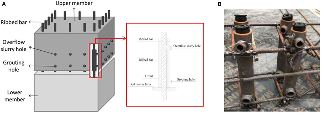
Figure 1. Full grouting sleeve connection. (A) Schematic diagram. (B) Physical diagram.

To form the joints, two steel bars were inserted into the sleeve, one from each end. The upper and lower longitudinal ribs extended into the sleeve by 120 and 110 mm, respectively. The special grout was then poured in via the grouting hole and flowed out from the overflow slurry hole until the sleeve was filled. In this situation, the hardened grout grips both the steel bar and the sleeve, and due to its micro-expansion and high strength characteristics, the positive force between the sleeve and the steel bar is strengthened (Zheng et al., 2015).

The construction of a full grouting sleeve is very complicated, and during the construction process, sleeve defects, such as grout leakage, eccentricity of the steel bars, incomplete fill of grout, and peeling of the grout from the connecting members are usually inevitable. Grout sleeve bond failure is a typical but undesirable failure mode in grout sleeve joints. Grout sleeve defects will seriously affect the mechanical properties of the joint, becoming a potential risk to the structure. Figure 2 shows an incomplete fill of grout sleeve defect caused in on-site construction, and it is the most common defect type in actual engineering.

FIGURE 2

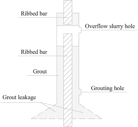
Figure 2. Incomplete fill of grout sleeve defect caused in on-site construction.

CNN-Based Defect Identification Method

This study presents a defect identification method for prefabricated concrete structures based on a deep convolutional neural network. This network can directly extract defect features from the dynamic response of the fabricated concrete structure. An overview of the proposed method is shown in Figure 3 and is described briefly as follows: (1) An experiment is conducted to obtain acceleration response data for the fabricated concrete structure; (2) the collected dynamic response data are preprocessed, data sets (training, validation and test sets) are established, and the samples are labeled; (3) a deep CNN, as shown in Figure 4, is trained on the training data set; (4) the loss of validation during the training process was calculated for each epoch to test whether it is over fitting; (5) the test set is used to verify the feasibility and accuracy of the CNN; (6) Defect location and degree were identified.

FIGURE 3

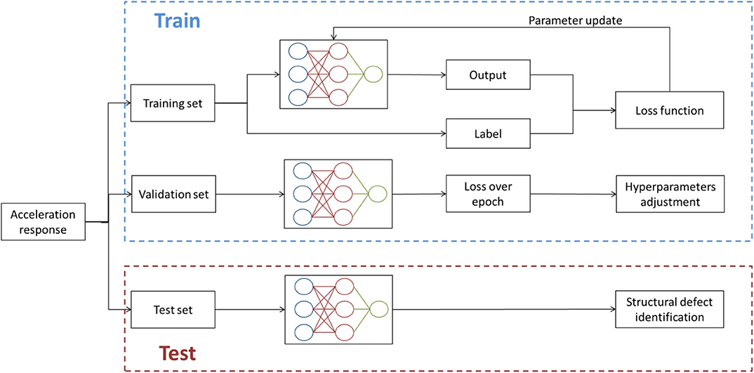
Figure 3. The process of structural defect identification based on a CNN. Here, defect probability represents that the output was mapped into a probability distribution in the range [0, 1] through the Softmax function.

FIGURE 4

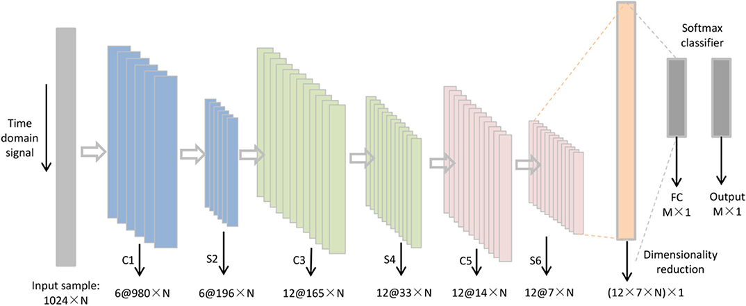
Figure 4. Basic framework of the CNN. Here, C represents a convolution layer, S represents a pooling layer, FC represents the fully connected layer, N represents the number of nodes in the input sample, and M represents the number of nodes in the output.

The deep learning network is established based on LeNet-5 (LeCun et al., 1989), a CNN that is famous for its simple structure and high efficiency. The Matlab toolkit DeepLearnToolbox was employed to establish the proposed CNN architecture. DeepLearnToolbox is the most widely used deep learning toolkit in Matlab, and the CNN in this toolkit was built by Rasmus Berg Palm on the basis of LeNet-5. In a recognition test of the Modified National Institute of Standards and Technology database, an error rate of 1.22% was obtained. The proposed deep CNN basic framework is shown in Figure 4. It can be seen that the CNN consisted of an input layer, three alternating convolutional and pooling layers, a fully connected layer, and an output layer. The components of the CNN and the selection of the activation function and optimization algorithm are described in the next sections.

Convolution Layer

The convolution layer is the core of the CNN, and its purpose is to use a convolution kernel to extract signal features. Generally, convolution is a mathematical operation on two real variable functions. The convolution expression of functions x and w can be calculated as

$\begin{array}{ll}s(t)=\int x(a)\times w(t-a)da& (1)\end{array}$

The discrete form of this convolution operation can be defined as

$\begin{array}{ll}s(t)=(x*w)(t)=\sum x(a)w(t-a)& (2)\end{array}$

In general, the first parameter in the convolution operation is called the input, the second parameter is called the convolution kernel, and the output is called a feature map. According to the convolution expression, each element in the output is obtained by the weighted addition of the elements of the corresponding block in the input, and the weight value is determined by the convolution kernel. The convolution kernel therefore plays the role of filtering or feature extraction in the convolution. Convolutional layers have powerful feature-learning capabilities. In general, deep networks can continuously and iteratively extract higher-level features from the features of the underlying network.

Activation Function

Generally, a convolutional layer is followed by a non-linear activation function. The activation function maps the linear input data into non-linear features through its own non-linear features, and the features obtained in the convolutional layer are filtered. Common non-linear functions in convolutional neural networks include the sigmoid, tanh, softsign, and ReLU functions (Zhou and Mi, 2017). Generally, the performance of the ReLU function is considered best. In this study, the defect identification accuracies obtained using tanh and ReLU functions with different learning rates of 0.005, 0.01, 0.02, and 0.05 were compared using experimentally obtained sensing acceleration response data. The results are shown in Table 1, and these show that the identification accuracy of the tanh function in this example is significantly better than that of the ReLU function. Therefore, the tanh function was selected as the activation function of the convolutional layer in the CNN. An expression for the tanh function is shown in Equation (3).

$\begin{array}{ll}y=\frac{e^x-e^{-x}}{e^x+e^{-x}}& (3)\end{array}$

TABLE 1

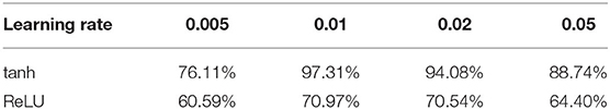
Table 1. Identification accuracy for tanh and ReLU activation functions with different learning rates.

Pooling Layer

Pooling is mainly used to filter redundant features and reduce the number of parameters, avoiding over-fitting. There are two common pooling operations: maximum pooling and average pooling. Maximum pooling takes the maximum value of each pooling window and average pooling takes the average value of each pooling window. In this work, the average pooling method was used. The average pooling operation is shown in Figure 5.

FIGURE 5

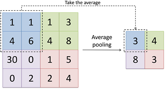
Figure 5. The average pooling operation.

Fully Connected Layer and Softmax Classifier

The fully connected layer is connected to all the activations in the previous layer. In this work, all the elements in the feature map of pooling layer S6 were processed into an M-dimensional column vector, multiplied by weighting coefficients, and added with corresponding offsets. The softmax function was then used to calculate the final output of the CNN. The softmax function can be expressed as

$\begin{array}{ll}{S}_i=\frac{e^{V_i}}{{\displaystyle \sum _{i=1}^C}{e}^{V_i}}& (4)\end{array}$

where S_i is the probability that the current input is the i-th category, e is Euler's number, V_i is the i-th output of the previous output unit, and C is the total number of categories. As shown in Equation (4), the softmax classifier maps the output of the previous output unit to the interval (0, 1), and this represents the relative probabilities of different categories so that the input samples can be classified according to their probability.

Batch Gradient Descent Algorithm

In the calculation process of the backpropagation algorithm, the parameters in the CNN need to be optimized to minimize the cost function to obtain an optimal solution. In this work, a cross-entropy cost function was used. The cross-entropy cost function can be expressed as

$\begin{array}{ll}E=-\frac{1}{N}\left(y^{(i)}\times \text{ln}(o^{(i)})+(1-y^{(i)})\times \text{ln}(1-o^{(i)})\right)& (5)\end{array}$

where E represents the cost function value, N represents the total number of samples, y⁽ⁱ⁾ represents the true output (label) of the i-th sample, and o⁽ⁱ⁾ represents the predicted output of the i-th sample. The small-batch gradient descent algorithm was used as the optimization algorithm. As shown in Table 1, in this example, the identification accuracy is better when the learning rate is 0.01, so the learning rate was set as 0.01 in the batch gradient descent algorithm.

Experimental Verification

To verify the accuracy and feasibility of the proposed deep learning method, dynamic excitation tests were carried out on a prefabricated half-scaled, two-floor concrete frame with different defective columns.

Experimental Model

A half-scaled, two-floor prefabricated concrete frame structure was constructed. This mainly comprised four parts: precast columns, precast beams, precast foundation beams, and a poured concrete slab. The beams and columns were made from concrete, the standard value of compressive strength of concrete cube is 30 N/mm. Longitudinal reinforcements and stirrups were made from hot-rolled ribbed bars with a standard value of yield strength of 400 MPa and a modulus of elasticity of 200 GPa. The full grouting sleeve connection method was used to splice the internal reinforcements in the foundation beams and columns. A plan of the column net in this experimental model is shown in Figure 6A, and elevation views are shown in Figure 6B. Total 48 grouting connections were used in this frame structure model. The grouting process is shown in Figure 7.

FIGURE 6

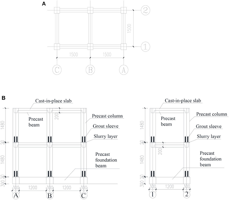
Figure 6. Plan and elevation views of the frame model. (A) Plan view of the column net of the frame model. (B) The A–C and 1–2 elevation views of the frame model.

FIGURE 7

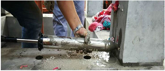
Figure 7. The grouting process.

In this test, precast beam and column members were manufactured by professional prefabricated assembly member manufacturing plants, and they were assembled in the laboratory of Tongji University after curing. The frame structure model after assembly is shown in Figure 8.

FIGURE 8

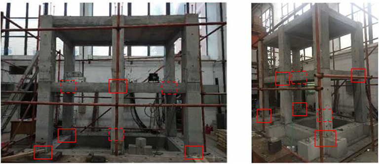
Figure 8. Frame structure model after assembly. Red rectangles represent locations of defects (the dashed lines indicate that they are shaded).

Defect Setting

In these experiments, defects in grout sleeve joints are introduced through incomplete grouting. To avoid structural damage to or collapse of the structure, the defects were arranged in the precast columns of the second floor instead of the first floor. As shown in Figure 9, for comparative analysis, defects were set only on one of the columns on either side of a particular beam. Excitation points were arranged across the span of the beams. Thus, for the same excitation, both defective column vibration responses and non-defective column vibration responses could be obtained.

FIGURE 9

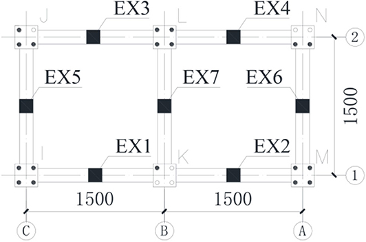
Figure 9. Defect setting of the second floor and excitation point arrangement. Solid dots represent grouting sleeves and hollow dots represent ungrouted sleeves. EX represents the excitation point location.

As shown in Table 2, there were seven working conditions corresponding to seven excitation points. Taking working condition 5 as an example, 14 measuring points were arranged for each working condition. The locations and numbers of excitation points and measuring points are shown in Figure 10.

TABLE 2

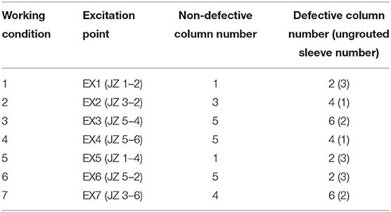
Table 2. Working conditions.

FIGURE 10

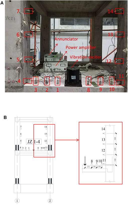
Figure 10. Arrangement of the excitation points and measuring points. (A) Physical diagram. (B) Schematic diagram.

Results and Discussion

Data Collection

Excitation was applied by vibration exciters, and acceleration sensors were arranged at the measuring points to collect acceleration responses. The excitation force was 200 N and the acquisition frequency was 1,024 Hz. Each excitation point is excited once, and the duration of excitation is 60 s.

According to the acceleration time-history curve analysis, the amplitude at each measuring point in each working condition was different. For the stability of the convolutional neural network during the training process, a normalization layer is added to the proposed network (Dorafshan and Azari, 2020). The amplitudes of the acceleration time-histories are normalized as

$\begin{array}{ll}{y}_i=\frac{x_i}{{\displaystyle \underset{i=1,2,\cdots ,N}{max}}(|x_i|)}& (6)\end{array}$

where x represents the original acceleration time history, y represents the acceleration time history after the amplitude is normalized, and i is the index of each measuring point.

The acceleration time history from each measuring point was taken as the input sample. For each working condition, 14 acceleration time histories were obtained. As shown in Figure 11, the 60 × 1,024 signals of each measuring point were divided into 5,000 parts. Each part includes 1,024 signals and adjacent parts have an overlap of 1,012 signals. The first seven acceleration time histories were collected from the columns and beams without defects and constituted the non-defective sample; the last seven acceleration time histories were collected from the defective columns and beams and constituted the defective sample. That is, there are in total 5,000 non-defective samples and 5,000 defect samples for each working condition, and each sample contains 7 × 1,024 acceleration signals. Sixty percentange of the total samples were randomly selected as the training set, 20% of the samples were selected randomly as validation set, with the remaining 20% constituting the test set.

FIGURE 11

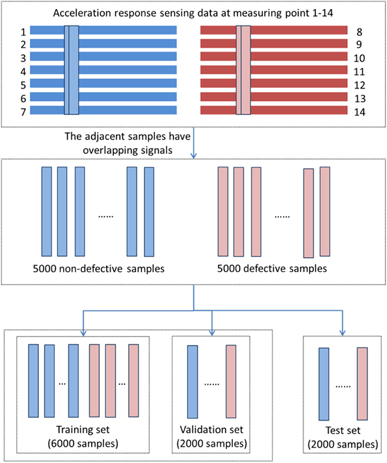
Figure 11. The creation of datasets.

The number of training set samples generated in this experiment was relatively small. The batch size was therefore set to five to ensure that there were a sufficient number of samples for training; the epoch number was set to 20. The number of iterations can be calculated as

$\begin{array}{ll}IN=EN\times \frac{TS}{BS}& (7)\end{array}$

where IN represents the number of iterations, EN represents epoch number, TS represents the training set size, and BS represents the batch size.

Defect Location Identification

The defects and their locations were identified for the samples in each working condition. The samples were labeled with a vector consisting of eight elements. The first seven elements represent the probability that a defect is located at each of the seven corresponding measurement points. The eighth element represents the probability that the sample is a non-defective sample. In this experiment, a defect was set at measuring point 4, so the label of the defective sample was [0, 0, 0, 1, 0, 0, 0, 0]; the label of the non-defective sample was [0, 0, 0, 0, 0, 0, 0, 1]. Thus, the sample is identified as a defective sample when the fourth element in the sample output vector is > 0.95, the sample is identified as a non-defective sample when the eighth element in a sample output vector is >0.95, and the identification is invalid when no element in a sample output vector is > 0.95. Based on the above label setting, the detailed parameters for each layer in the CNN are shown in Table 3.

TABLE 3

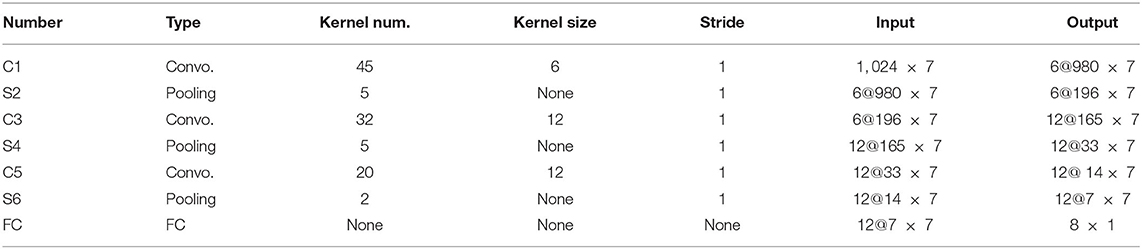
Table 3. Detailed parameters of each layer in the CNN.

As shown in Figure 12, during the training process, the loss function in the CNN gradually decreased with an increasing number of iterations and converged to a stable level for each working condition. As shown in Figure 13, the loss of validation during the training process was calculated for each epoch to test whether it is over fitting, and the training stopped in the 20th epoch (the loss of validation was not changed significantly). The identification accuracies for each working condition during the training process of the CNN are shown in Figure 14. It can be seen that during the CNN training process, the identification accuracy rate of samples in the seven working conditions continuously increased with the growth of the epochs, and finally stabilized at 100%. The four longitudinal working conditions (conditions 1–4) converged faster than the three lateral working conditions (conditions 5–7).

FIGURE 12

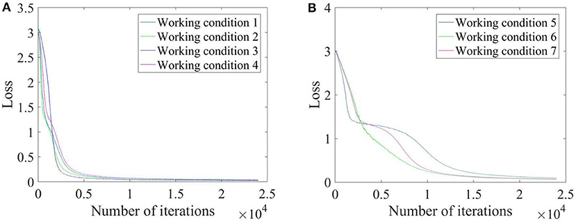
Figure 12. The loss functions for each working condition during the CNN training process. (A) Working conditions 1–4. (B) Working conditions 5–7.

FIGURE 13

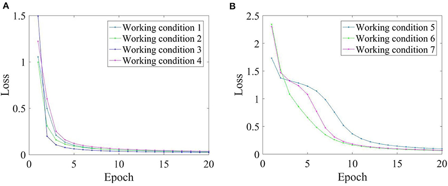
Figure 13. Losses of validation for each working condition during the CNN training process. (A) Working conditions 1–4. (B) Working conditions 5–7.

FIGURE 14

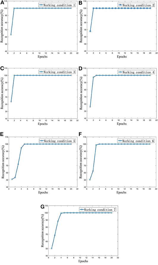
Figure 14. The identification accuracies of seven working conditions during the CNN training process. (A) Working condition 1. (B) Working condition 2. (C) Working condition 3. (D) Working condition 4. (E) Working condition 5. (F) Working condition 6. (G) Working condition 7.

For each working condition, 2,000 test samples were sequentially input into the trained convolutional neural network. The test results showed that the identification accuracies of the seven test sets were all 100%. This means that the proposed method can successfully identify defects and their locations.

Defect Degree Identification

For defect degree identification, the precast defective columns of working conditions 5, 6, and 7 have covered the defect degrees of 25, 75, and 50% with the same boundary conditions in the test. So these three working conditions (5, 6, and 7) were taken as this section's research object. There were in total 15,000 samples, 60% of these were randomly selected as the training set, 20% of the samples were selected as validation set, with the remaining 20% constituting the test set. The batch size was set to five, and the epoch number was set to 20.

The sample labels were vectors consisting of three elements. The first element represents the defect degree being 25%, the second element represents the defect degree being 50%, and the third element represents the defect degree being 75%. For example, a sample label with 25% defect degree would be [1, 0, 0].

To realize the identification of the defect degree, the difference between the sample output vector and the sample label vector is calculated using the Euclidean distance (Schnitzer et al., 2012). The Euclidean distance ρ between two points (x₁, x₂, …, x_n) and (y₁, y₂, …, y_n) in n-dimensional space can be calculated from

$\begin{array}{ll}\rho =\sqrt{{(x_1-y_1)}^2+{(x_2-y_2)}^2+\cdots +{(x_n-y_n)}^2}& (8)\end{array}$

A confusion matrix is used to measure the classification and prediction ability of the model (Thongkam et al., 2008). The identification result of a sample can be one of four types, as shown in Table 4: true positive (TP), false positive (FP), false negative (FN), and true negative (TN). The precision ratio (p) and recall ratio (r) of the confusion matrix can be calculated from

$\begin{array}{ll}p=\frac{TP}{TP+FP}& (9)\end{array}$

$\begin{array}{ll}r=\frac{TP}{TP+FN}& (10)\end{array}$

During the training process, the losses of train and validation are shown in Figure 15. Three samples (from three working conditions) were randomly selected from the test set. The Euclidean distances between the output vectors and the sample labels are shown in Table 5. Test samples were sequentially input into the trained convolutional neural network, and the confusion matrix of the identification results is shown in Table 6. This table shows that both the precision ratio and the recall rate for each sample type were 100%. The evaluation target of precision ratio is the prediction results, the number of positive samples among the samples whose prediction is positive. The precision ratio is 100%, indicating that the prediction results of all samples with different defect degrees are positive. The evaluation target of recall ratio is the original samples, the number of positive examples that are predicted correctly. The recall ratio is 100%, indicating that all the samples with different defect degrees have been predicted correctly. Table 6 shows that the CNN is stable and has good identification performance for structural defect identification in a prefabricated frame. There was no significant difference between the recall rate and the accuracy rate, indicating that the CNN does not show bias toward different defect types.

TABLE 4

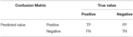
Table 4. Confusion matrix.

FIGURE 15

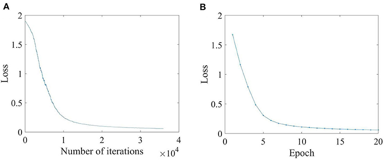
Figure 15. The train and validation losses during the CNN training process. (A) Train losses over iterations. (B) Validation losses over epochs.

TABLE 5

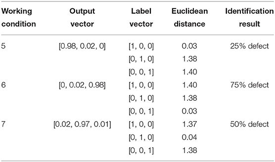
Table 5. Euclidean distances between the output vectors and the sample labels.

TABLE 6

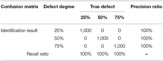
Table 6. Confusion matrix of the identification results.

Conclusions

This paper presented a deep-CNN-based method for identification of sleeve joint defects in prefabricated concrete frame structures. The proposed method uses LeNet-5 as the basic framework and refers to the CNN in the DeepLearnToolbox. Non-destructive dynamic tests on a half-scaled, two-floor prefabricated concrete frame structure were carried out. The CNN was trained using only the collected sensing acceleration responses to extract features for sleeve joint defect identification. In the experiment, there were seven working conditions due to the different defect degrees and boundary conditions. For each working condition, 5,000 non-defective samples and 5,000 defective samples were collected, and 60% of these were selected randomly as the training set, 20% of these were selected as validation set, while the remaining 20% were used to test the CNN. The defects and their locations were identified using the CNN, and the identification accuracy was 100% in each working condition. The Euclidean distances between the output vectors and the label vectors were calculated to determine the defect identification result, and a confusion matrix was used to judge the identification accuracy. Defects with different degrees were identified in lateral working conditions 5, 6, and 7. The results showed that both the precision ratio and the recall rate were 100%, and the proposed method did not show bias toward different defect degrees. Overall, the proposed method was found to be very effective in joint defect identification in prefabricated concrete frame structures in the experimental situation examined in this paper.

Data Availability Statement

The raw data supporting the conclusions of this article will be made available by the authors, without undue reservation. Raw data are provided in the Supplementary Material.

Author Contributions

HT, TZ, YX, and SX: methodology. TZ: software. HT and SX: supervision. YX: validation and writing—original draft. HT, YX, and SX: writing—review and editing. All authors read and agreed to the published version of the article.

Funding

This research was funded by the Ministry of Science and Technology of China (grant number SLDRCE19-B-02) and the National Key R&D Program of China (grant numbers 2017YFC0703600 and 2016YFC0701800).

Conflict of Interest

The authors declare that the research was conducted in the absence of any commercial or financial relationships that could be construed as a potential conflict of interest.

Supplementary Material

The Supplementary Material for this article can be found online at: https://www.frontiersin.org/articles/10.3389/fmats.2020.00298/full#supplementary-material

References

Abdeljaber, O., Avci, O., Kiranyaz, M. S., Boashash, B., Sodano, H., and Inman, D. J. (2018). 1-D CNNs for structural damage detection: Verification on a structural health monitoring benchmark data. Neurocomputing 275, 1308–1317. doi: 10.1016/j.neucom.2017.09.069

CrossRef Full Text | Google Scholar

Abdeljaber, O., Avci, O., Kiranyaz, S., Gabbouj, M., and Inman, D. J. (2017). Real-time vibration-based structural damage detection using one-dimensional convolutional neural networks. J. Sound Vib. 388, 154–170. doi: 10.1016/j.jsv.2016.10.043

CrossRef Full Text | Google Scholar

Avci, O., Abdeljaber, O., Kiranyaz, S., Hussein, M. F., Gabbouj, M., and Inman, D. J. (2020). A review of vibration-based damage detection in civil structures: from traditional methods to machine learning and deep learning applications. arXiv:2004.04373. doi: 10.1016/j.ymssp.2020.107077

CrossRef Full Text | Google Scholar

Beckman, G. H., Polyzois, D., and Cha, Y. J. (2019). Deep learning-based automatic volumetric damage quantification using depth camera. Autom. Constr. 99, 114–124. doi: 10.1016/j.autcon.2018.12.006

CrossRef Full Text | Google Scholar

Cha, Y. J., Choi, W., and Büyüköztürk, O. (2017). Deep learning-based crack damage detection using convolutional neural networks. Comp.-Aided Civil Inf. Eng. 32, 361–378. doi: 10.1111/mice.12263

CrossRef Full Text | Google Scholar

Chen, M., Tang, Y., Zou, X., Huang, K., Li, L., and He, Y. (2019). High-accuracy multi-camera reconstruction enhanced by adaptive point cloud correction algorithm. Opt. Lasers Eng. 122, 170–183. doi: 10.1016/j.optlaseng.2019.06.011

CrossRef Full Text | Google Scholar

China Institute of Building Standard Design and Research (2014). JGJ 1-2014. Technical Specification for Precast Concrete Structures. Beijing: China Construction Industry Press.

Google Scholar

Chou, H. C. (2019). Concrete object anomaly detection using a non-destructive automatic oscillating impact-echo device. Appl. Sci. 9:904. doi: 10.3390/APP9050904

CrossRef Full Text | Google Scholar

Dorafshan, S., and Azari, H. (2020). Evaluation of bridge decks with overlays using impact echo, a deep learning approach. Automat. Constr. 113:103133. doi: 10.1016/j.autcon.2020.103133

CrossRef Full Text | Google Scholar

Dorafshan, S., Thomas, R. J., and Maguire, M. (2018). Comparison of deep convolutional neural networks and edge detectors for image-based crack detection in concrete. Constr. Build. Mater. 186, 1031–1045. doi: 10.1016/j.conbuildmat.2018.08.011

CrossRef Full Text | Google Scholar

du Plessis, A., and Boshoff, W. P. (2019). A review of X-ray computed tomography of concrete and asphalt construction materials. Constr. Build. Mater. 199, 637–651. doi: 10.1016/J.CONBUILDMAT.2018.12.049

CrossRef Full Text | Google Scholar

Duan, Y., Chen, Q., and Zhang, H. (2019). CNN-based damage identification method of tied-arch bridge using spatial-spectral information. Smart Struct. Syst. 23, 507–520. doi: 10.12989/SSS.2019.23.5.507

CrossRef Full Text | Google Scholar

Feng, K., Zhao, Q., and Qiu, Y. (2020). Damage imaging in mesoscale concrete modeling based on the ultrasonic time-reversal technique. Acta Mech. Solida Sin. 33, 61–70. doi: 10.1007/s10338-019-00153-z

CrossRef Full Text | Google Scholar

Gao, R., Li, X., Liu, H., Xu, Q., Wang, Z., and Zhang, F. (2019). Experimental study on detecting sleeve grouting defect depth by embedded non-contact steel wire drawing hole-forming method. Constr. Technol. 48, 17–19. doi: 10.7672/sgjs2019090017

CrossRef Full Text | Google Scholar

Gao, R., Li, X., and Zhang, F. (2017). Testing test of sleeve grouting compactness based on X-ray industrial CT technology. Nondestruct. Test. 39, 6–11. doi: 10.11973/wsjc201704002

CrossRef Full Text | Google Scholar

Gulgec, N. S., Takáč, M., and Pakzad, S. N. (2019). Convolutional neural network approach for robust structural damage detection and localization. J. Comput. Civ. Eng. 33:04019005. doi: 10.1061/(ASCE)CP.1943-5487.0000820

CrossRef Full Text | Google Scholar

Khodabandehlou, H., Pekcan, G., and Fadali, M. S. (2019). Vibration-based structural condition assessment using convolution neural networks. Struct. Control Health Monit. 26:e2308. doi: 10.1002/STC.2308

CrossRef Full Text | Google Scholar

Kim, H., and Sim, S. H. (2019). Automated peak picking using region-based convolutional neural network for operational modal analysis. Struct. Control Health Monit. 26:e2436. doi: 10.1002/stc.2436

CrossRef Full Text | Google Scholar

LeCun, Y., Boser, B., Denker, J. S., Henderson, D., Howard, R. E., Hubbard, W., et al. (1989). Backpropagation applied to handwritten zip code recognition. Neural Computation 1, 541–551. doi: 10.1162/neco.1989.1.4.541

CrossRef Full Text | Google Scholar

Lee, S., Ha, J., and Zokhirova, M. (2018). Background information of deep learning for structural engineering. Arch. Comput. Methods Eng. 25, 121–129. doi: 10.1007/s11831-017-9237-0

CrossRef Full Text | Google Scholar

Li, X., Lin, Y., and Ma, H. (2018). Research on the application of bridge damage identification method based on convolutional neural network. J. Qinghai Univ. 2, 41–46. doi: 10.13901/j.cnki.qhwxxbzk.2018.02.007

CrossRef Full Text | Google Scholar

Lin, Y., Nie, Z., and Ma, H. (2017). Structural damage detection with automatic feature-extraction through deep learning. Comp.-Aided Civil Inf. Eng. 32, 1025–1046. doi: 10.1111/mice.12313

CrossRef Full Text | Google Scholar

Pathirage, C. S., Li, J., and Li, L. (2018). Structural damage identification based on autoencoder neural networks and deep learning. Eng. Struct. 172, 13–28. doi: 10.1016/J.ENGSTRUCT.2018.05.109

CrossRef Full Text | Google Scholar

Schnitzer, D., Flexer, A., Schedl, M., and Widmer, G. (2012). Local and global scaling reduce hubs in space. J. Mach. Learn. Res. 13, 2871–2902. doi: 10.1051/cocv/2012004

CrossRef Full Text | Google Scholar

Tang, Y., Chen, M., Wang, C., Luo, L., Li, L., and Zou, X. (2020). Recognition and localization methods for vision-based fruit picking robots: a review. Front. Plant Sci. 11:510. doi: 10.3389/fpls.2020.00510

PubMed Abstract | CrossRef Full Text | Google Scholar

Tang, Y., Li, L., Wang, C., Chen, M., Feng, W., Zou, X., et al. (2019). Real-time detection of surface deformation and strain in recycled aggregate concrete-filled steel tubular columns via four-ocular vision. Robot. Comput. Integr. Manuf. 59, 36–46. doi: 10.1016/j.rcim.2019.03.001

CrossRef Full Text | Google Scholar

Thongkam, J., Xu, G., and Zhang, Y. (2008). “AdaBoost algorithm with random forests for predicting breast cancer survivability,” in 2008 IEEE International Joint Conference on Neural Networks (IEEE World Congress on Computational Intelligence), 3062–3069. doi: 10.1109/IJCNN.2008.4634231

CrossRef Full Text | Google Scholar

Wang, Z., Zheng, H., and Li, L. (2019). Practical multi-class event classification approach for distributed vibration sensing using deep dual path network. Opt. Express 27, 23682–23692. doi: 10.1364/OE.27.023682

PubMed Abstract | CrossRef Full Text | Google Scholar

Xie, X., Shan, D., and Zhou, X. (2018). Bridge damage identification method based on stacked denoising autoencoders. Railw. Construct. 58, 1–5. doi: 10.3969/j.issn.1003–1995.2018.05.01

CrossRef Full Text | Google Scholar

Xu, Y., Wei, S., Bao, Y., and Li, H. (2019). Automatic seismic damage identification of reinforced concrete columns from images by a region-based deep convolutional neural network. Struct. Control Health Monit. 26, 1–22. doi: 10.1002/stc.2313

CrossRef Full Text | Google Scholar

Yoon, M. K., Heider, D., Gillespie, J. W., Ratcliffe, C. P., and Crane, R. M. (2010). Local damage detection with the global fitting method using operating deflection shape data. J. Nondestruct. Eval. 29, 25–37. doi: 10.1007/s10921-010-0062-8

CrossRef Full Text | Google Scholar

Yu, Y., Wang, C., Gu, X., and Li, J. (2019). A novel deep learning-based method for damage identification of smart building structures. Struct. Health Monitor. 18, 143–163. doi: 10.1177/1475921718804132

CrossRef Full Text | Google Scholar

Zelelew, H. M., Almuntashri, A., Agaian, S., and Papagiannakis, A. T. (2013). An improved image processing technique for asphalt concrete X-ray CT images. Road Mater. Pavement Des. 14, 341–359. doi: 10.1080/14680629.2013.794370

CrossRef Full Text | Google Scholar

Zhao, Y. (2019). Research on Blade Damage Identification Method Based on Convolutional Neural Network. Tianjin: School of Aeronautical Engineering, Civil Aviation University of China. doi: 10.27627/d.cnki.gzmhy.2019.000074

CrossRef Full Text | Google Scholar

Zheng, Y., Guo, Z., and Cao, J. (2015). Constraint mechanism and constraint stress distribution of new grout sleeve. J. Harbin Inst. Tech. 47, 106–111. doi: 10.11918/j.issn.0367-6234.2015.12.019

CrossRef Full Text | Google Scholar

Zhou, C., and Mi, H. (2017). A comparative study on the performance of three kinds of activation functions in deep learning. J. Beijing Institute Electron. Technol. 4, 27–32. doi: 10.3969/j.issn.1672-464X.2017.04.005

CrossRef Full Text | Google Scholar

Zhu, W., Gao, Z., and Huang, S. (2018). Research on testing technology of grouting plumpness of sleeve based on vibration amplitude of sensors method. Constr. Qual. 36, 7–10. doi: 10.3969/j.issn.1671-3702.2018.11.003

CrossRef Full Text | Google Scholar

Zhu, W., Xu, J., Zhang, H., Han, W., and Cai, Y. (2019). Common quality defects and repair methods of precast concrete members. Concrete 5, 115–118. doi: 10.3969/j.issn.1002-3550.2019.05.028

CrossRef Full Text | Google Scholar