Understanding the Impact of Machine Learning Models on the Performance of Different Flexible Strain Sensor Modalities

1 Introduction

The integration of electronics into clothing to make “smart textiles” is commonly used to track motion and aid rehabilitation, improve athletic training, prevent injury, recognize gestures, and acquire bio-signals (Fleury et al., 2015). The occurrence of wearable sensor research articles has increased on average 28% yearly over the past 10 years¹ and will likely continue to grow in popularity as electronics become smaller and more integrated. Advances in soft strain sensors that enable motion tracking have progressed recently to ever higher performance. The application of different sensor materials and principles of operation can have a large effect on the signal characteristics, for better or for worse. For example, accuracy suffers when tracking running at high speeds with some resistive sensor types (Mengüç et al., 2014). Others display high sensitivity but only over a limited strain range making them best suited for tracking fine movements—such as wearable sensors using capacitance to detect strain of finger joints for gesture detection (Liu et al., 2011; Lee et al., 2015; Kim et al., 2017). Sensor properties such as strain bandwidth, dynamic range, hysteresis, and static drift affect the tracking of movements where high speeds, large strains, cyclic motion, or prolonged static periods are expected, respectively. Quite often, these deleterious effects are inherent to the materials used to create the sensor and can be overlooked when focusing on advances such as gauge factor (GF) or maximum achievable strain with new sensor compositions or fabrication methods. An alternative strategy for improving sensing performance has been to implement machine learning (ML) algorithms to predict or classify movements or estimate body segment positions (Vu and Kim, 2018). Software models have also been used to correct and improve sensor signals in the presence of detrimental sensor properties, an approach that has been limited to three reports (Kim and Kim, 2017; Miodownik et al., 2019; Oliveri et al., 2019). The ability of machine learning to extract patterns from complex, nonlinear signals in the presence of disturbances like random noise and electromagntic interference (EMI) may be used to maximize the information gained from a sensor (Miodownik et al., 2019). It is important for future developments to determine the advantageous and limiting characteristics of each sensor technology and understand the possible improvements in signal fidelity realized when each type is combined with modelling. This enables designers to gain knowledge about which sensor is best suited for a specific type of motion tracking application, or simply to push forward sensing abilities from both hardware and software approaches.

Three modalities of fiber strain sensors may be distinguished by their mode of operation: using changes in resistance, capacitance, or inductance to transduce strain. Fibre sensors using the piezoresistive effect have been fabricated with conductive polymers, polymer-conductor composites, ionic liquids, liquid metals, and carbon nanotubes (Shin et al., 2010; Seyedin et al., 2015; Wu et al., 2016; Choi et al., 2017; Keulemans et al., 2017; Zahid et al., 2017; Chen et al., 2018). Sensor arrangement for integration into textiles may incorporate monofilaments, multifilament fibres, knitted textiles, or foams (Seyedin et al., 2015; Zahid et al., 2017; Jung et al., 2019; Yin et al., 2019; Zheng et al., 2019). Polymer-conductor composite (PC) sensors are commonly used in wearable applications because of their scalable manufacturing processes, high sensitivity, and ease of interfacing with textiles and electronics (Liu et al., 2018a). Many factors (see Supplementary Equation S1 for details) influence the piezoresistance of the polymer including mechanical polymer properties, conductive filler choice and distribution, mode of conduction, and the presence of micro-cracks between conductive regions (Stübler et al., 2011; Liu et al., 2018a).

The combination of effects that contribute to a sensor’s resistance causes its signal to diverge from an ideal linear strain-resistance relationship. The most obvious of these effects is a varying GF across the working strain range (He et al., 2019). A repeatable nonlinear signal response to strain is not necessarily detrimental for strain sensing because an operating point can be chosen around which the sensor signal is approximately linear, or the nonlinearity can be compensated for in software (Oliveri et al., 2019). Even simple regression models are able to easily handle repeatable signal nonlinearities. Mechanically, thermoplastic elastomers (TPE), pristine or composite, may posses hysteresis, strain softening, and fading memory in their stress-strain relationships (Diani et al., 2009; Drozdov and Dusunceli, 2014). Analogous electrical effects are often observed in TPE conductive composites including signal hysteresis, dynamic drift, and static drift (Clemens et al., 2012). Signal hysteresis occurs when the sensor resistance is path dependent over a long number of cycles, having different resistance values for a given strain during extension and recovery (De Focatiis et al., 2012). Hysteresis modelling for composite sensors and geometrical modifications of the ionic liquid type have been used to compensate for and reduce hysteresis (Choi et al., 2017; Kim and Kim, 2017). Dynamic drift refers to a transient change in the resistance when exposed to cyclic strain that decays to a steady-state (De Focatiis et al., 2012). Static drift in resistance during constant strain is attributable to polymer stress relaxation (Kalantari et al., 2012). The readout electronics for piezoresistive sensors may be as simple as a voltage divider circuit with one analog-to-digital converter (ADC). In addition, high sensitivities (GF > 1,000) are achievable while maintaining maximum strain in excess of 100% (He et al., 2019).

Soft sensors that use capacitance to measure strain are advantageous because they greatly reduce the dependency of GF on strain when compared to the piezoresistive type. This is due to the underlying mechanism of capacitance modulation relying only on a change in geometry (see Supplementary Equations S2, S3 for details). Capacitive sensors have been fabricated from liquid metal in tubes, polymer composites, and thin film electrodes in parallel plate, coaxial, and twisted-pair configurations (Frutiger et al., 2015; Lee et al., 2015; Wang et al., 2016; Cooper et al., 2017; Kim et al., 2017). The relative change in capacitance limits ideal capacitive sensors of this construction to unity gauge factor. A difficulty associated with capacitive sensors is the complex measurement electronics necessary to read capacitance. Whereas resistive sensors can be read with minimal electronic components, capacitive sensors require AC excitation and precise timing to measure. Conductive polymer electrodes have their own piezoresistive effect that manifests as a strain-dependent equivalent series resistance (ESR) to the measurement circuit (Michel et al., 2012; Liu et al., 2015). High ESR hinders the rate at which a capacitive sensor may be sampled and limits the strain frequencies that are measurable. Manufacturing is more complex than piezoresistive sensors because at least three layers are required—two electrode layers with electrical connections that must remain isolated by a dielectric layer—becoming difficult to manufacture at scale. Eliminating short circuits between electrodes and accessing the inner electrode in a downsized coaxial fibre are non-trivial pursuits. Coupling capacitive sensors with modelling has been limited to developing mathematical models to predict its electrical behaviour (Frutiger et al., 2015). Combining ML models with capacitive sensors has the potential to compensate for strain-depedent ESR and improve measurement at high strain rates.

Inductive strain sensors are under-represented in comparison to piezoresistive and capacitive strain sensors. The inductive sensing modality has utilized inductance of a single loop, mutual inductance between loops positioned on different body segments, or the gain between receiver and transmitter antenna coils on various segments to track relative motion (Wijesiriwardana, 2006; Laskoski et al., 2009; Sardini et al., 2012; Patron et al., 2016). The inductance of a solenoid coil is dependent on its number of turns, cross-sectional area, and total wire length. One approach to single coil sensors is to rely on the change of area of a stretchable solenoid loop to measure strain, similar to inductance plethysmography systems (Zhang et al., 2012). Like the capacitive sensor, the inductive signal is directly dependent on geometry. However, this relationship is not linear. For a sensor with a reasonable length, the logarithmic behaviour with respect to length is negligible and sensor response can be linearly approximated as the GF (Tavassolian et al., 2020). According to Supplementary Equation S4, the number of perimeter loops does not influence the sensitivity but rather scales the baseline inductance allowing higher signal-to-noise ratio. One challenge with inductive sensors in wearable applications is rejecting electromagnetic interference (EMI) from the environment. Furthermore, the inductive loops must enclose a larger, rectangular area on the garment as opposed to the thread-like piezoresistive and coaxial capacitive designs. The aspect ratio varies during actual use and the sensor is not specific to uniaxial strain. Competing effects (i.e., Poisson effect) of decreasing width and increasing length when stretching along only one axis causes the sensor to have lower sensitivity than expected because the inductive signal is proportional to total area.

Herein, the performance of several ML models of increasing complexity are investigated when they are paired with different sensor types. The baseline performance of the sensors are compared with and without predictive modelling to examine its effect on strain-signal accuracy and how this would translate to wearable devices. The use of ML to compensate for undesirable sensor effects is explored and future areas of research to improve sensor design and performance are proposed. The performance of the sensors and ML models is probed by utilizing a random strain pattern that can be both visualized and statistically analyzed for performance improvements. Thus, by taking advantage of the computing power available in modern low-cost microcontrollers, ML may enable the use of simpler sensors and electronics with accuracy and range not yet realized.

2 Materials and Methods

2.1 Strain Sensor Fabrication

Two piezoresistive strain sensors, a capacitive, and an inductive sensor were used in this study. Each of these sensors are fiber-based to enable integration into textiles for quantitative motion tracking. The piezoresistive and capacitive sensors were produced using the same conductive composite of Hytrel 3078 (DuPont; Kingston, ON, Canada) and carbon black. Two different core filaments [Hytrel 3078 (H3078) monofilament and polyether urethane-urea (PEU) multifilament fiber] were used to understand the differences that mechanical supports have in affecting the piezoresistive signal. The inductive sensor was composed of an elastic fiber and coiled copper wire—it did not include any conductive composite. The sensors were fabricated as follows:

2.1.1 H3078-Core Piezoresistive Sensor (R-H3078)

A sensor with a piezoresistive sheath around a TPE core (R-H3078) was fabricated as described previously (Rezaei et al., 2019). A filament of H3078 TPE was extruded and dip coated once into a 50 wt% solution of H3078 and carbon black (Cabot Vulcan XC-72R; Alpharetta, GA, United States) in dichloromethane (5 wt% w.r.t. H3078) producing a fibre with 450 μm diameter, as shown in Figure 1A. The sensor samples were conditioned by subjecting them to 100 repeated cycles of stretching from 0–40% strain on a linear stage. The R-H3078 sensor had an unstrained specific resistance of $1.3\mathrm{k\Omega \; c}{\mathrm{m}}^{-1}$.

FIGURE 1

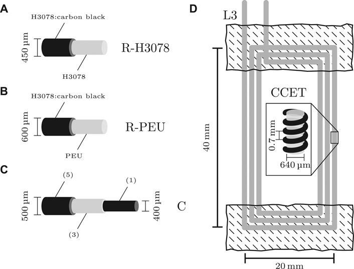
FIGURE 1. (A) Schematic of the R-H3078 sensor, consisting of extruded TPE core (grey) and dip-coated piezoresistive sheath (black). (B) Schematic of the R-PEU sensor consisting of PEU core filament (grey) and dip-coated piezoresistive sheath (black). (C) Schematic of the C sensor consisting of conductive core electrode (referred to as (1) in text), dielectric layer (3), and outer conductive electrode (5). The intermediate layers referenced in the text as (2) and (3) are not shown. (D) Schematic of the L3 inductive patch sensor containing three perimeter loops (thick grey), fabric backing (hatched area), and close-up inset of the CCET with copper wire (black) coiled around an elastic thread (grey).

2.1.2 PEU-Core Piezoresistive Sensor (R-PEU)

A second type of sensor with a piezoresistive sheath around a PEU core (R-PEU) was fabricated as described previously (Rezaei et al., 2019). A mixture of 50 wt% H3078 and carbon black in dichloromethane (5 wt% w.r.t. H3078) was used to dip coat a multifilament Dorlastan PEU fibre (Asahi Kasei; Düsseldorf, Germany) once, resulting in a final diameter of 600 μm (Figure 1B). These sensor samples were also conditioned by subjecting them to 100 repeated cycles of stretching from 0–40% strain. The R-PEU sensor had an unstrained specific resistance of $82\mathrm{\Omega \; c}{\mathrm{m}}^{-1}$.

2.1.3 Coaxial Capacitive Sensor (C)

A capacitive sensor (C) was produced as previously described (Geng et al., 2020). H3078 was extruded at 190°C to a diameter of 400 μm. The filaments were cut into 5 cm samples and dip-coated with a total of five layers: 1) 50 wt% H3078/carbon black in dicholormethane (5 wt% w.r.t. H3078); 2) polystyrene-ethylene-co-butylene-styrene (SEBS) in hexanes (5 wt%); 3) H3078 in dichloromethane (5 wt%); 4) SEBS in hexanes (5 wt%); 5) 50 wt% H3078/carbon black in dichloromethane (5 wt% w.r.t. H3078). Between dip-coating steps 1) and 2) the filament was inverted to ensure the inner electrode was accessible for electrical connection. Each dip-coated layer was allowed to dry before the next layer was added. After layer 5) was added, the sensors were put into a vacuum oven overnight at 60°C to ensure all volatiles were removed. The final diameter of the sensor was 500 μm (Figure 1C). The C sensor had an unstrained specific capacitance of $2.8\mathrm{pF\; c}{\mathrm{m}}^{-1}$.

2.1.4 Inductive Patch Sensor (L3)

An inductive sensor with three perimeter loops (L3) was fabricated as described in previous work (Tavassolian et al., 2020). Copper wire was coiled around a spandex elastic thread (diameter: 640 μm) using a custom-built machine to form a copper-coiled elastic thread (CCET). The feed rate of the thread was adjusted to obtain a helical coil with a pitch (spacing between coils) of 0.7 ± 0.1 mm. The CCET was then arranged in a rectangular pattern of three perimeter loops with approximate width of 2 cm and length of 4 cm. Rectangles of fabric backing were sewn along the width segments to provide a gripping surface for testing. The inner area of the sensor had an air gap. A schematic of this type of sensor is shown in Figure 1D. The L3 sensor had an unstrained specific inductance of $52\mathrm{nH\; c}{\mathrm{m}}^{-1}$ in the length direction.

2.2 Experimental Set-Up

The experimental set-up, shown in Figure 2, consisted of one of the four sensor types (exposed length: 37.35 ± 5.36 mm) mounted vertically in an Instron E10000 universal testing machine (UTM) (Instron; Norwood, MA, United States). A layer of electrical tape provided an even clamping force and insulated the sensors from the metal holding jaws. A strip of copper foil tape was used to connect the sensor electrodes to external electrical connections. The UTM used a 10 kN load cell sampling at 100 Hz and was subjected to linear displacement only (no torsional displacement).

FIGURE 2

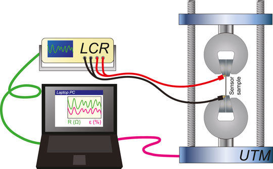
FIGURE 2. A schematic of the experimental set-up, consisting of a universal testing machine (UTM) driven to strain a sensor sample, inductance-capacitance-resistance (LCR) meter for sensor measurement, and laptop PC to control the UTM and log the resulting strain and sensor signal data.

Specimens were positioned in the clamps with approximate lengths of 40 mm, and the UTM cross head was retracted until the samples were just taut with minimal strain. The sensor length was manually measured and used as the reference length for 0% strain, ${\ell }_0$. For each test, the UTM was programmed to follow preprogrammed displacement profiles. These profiles were scaled relative to ${\ell }_0$, ensuring consistent strain among sensor samples.

The electrical response of each sensor, regardless of modality, was acquired by an Agilent E4980A precision inductance-capacitance-resistance (LCR) meter (Agilent; Santa Clara, CA, United States) with four-lead probe. The meter was configured in the mode suitable for the corresponding sensing modality and interfaced with a PC using a custom MATLAB script (The Mathworks; Natick, MA, United States). For each test, the raw impedance (resistance, capacitance, or inductance, denoted as Z) was normalized to its value at zero strain, $Z_0$ and expressed as the ratio $Z-Z_0/Z_0$. Mechanical data from the UTM was converted to strain $\epsilon =\ell -{\ell }_0/{\ell }_0$ and down-sampled to match the 55 Hz LCR sampling frequency.

3 Results

3.1 Tensile Stress-Strain Curve

Samples were subjected to a stress-strain test from 0–100% strain at a strain rate of 1%/s. The purpose of this test was to quantify the gauge factor, linearity, and working strain region. Plastic deformation was observed for all four specimens upon return from the strain cycle. The R-H3078 sensor elongated by 9.6%, the R-PEU sensor by 7.0%, the C sensor by 21.7%, and the L3 sensor by 1.9% compared to their pre-test length. The yield point of these thermoplastic elastomers was not abrupt and was observed as a gradual change in slope (Figure 3A). The elastic region, and therefore the working region, was previously found to be <30% strain for the piezoresistive fibres and this range was reasonable for use with all the sensor types (Rezaei et al., 2019). Within the working region, the Young’s modulus (stiffness) for the R-H3078, R-PEU, C, and L3 sensor types was 7.4, 6.9, 13.6, and 0.94 MPa, respectively. Stress and therefore stiffness for the L3 sensor was computed per fibre, of which there were six in parallel mechanically in the three-loop configuration.

FIGURE 3

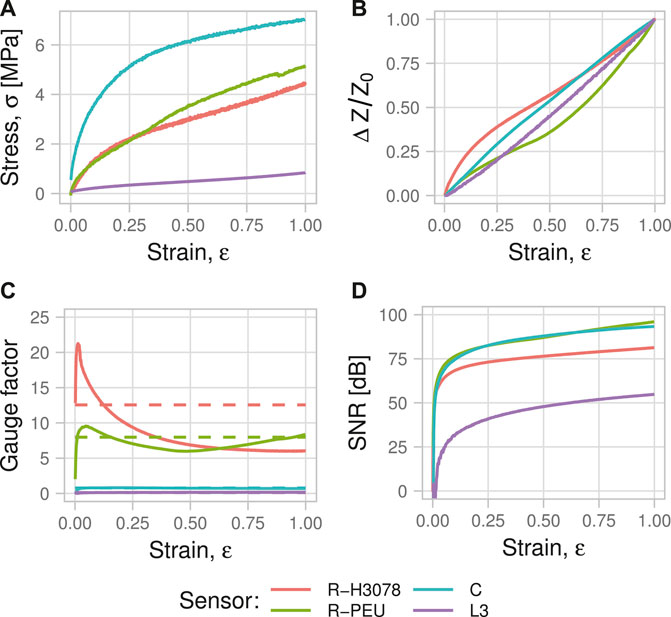
FIGURE 3. (A) Mechanical stress-strain curves for each sensor, (B) sensor output signal during the elongation, (C) instantaneous (solid) and average (dashed) gauge factor, (D) signal-to-noise ratio.

The linearity in the working strain range was measured by the coefficient of determination (R²) between the strain and the $\text{Δ}Z/Z_0$ signal scaled to the range $\left[\mathrm{0,1}\right]$. The R-H3078, R-PEU, C, and L3 sensors had R² values 0.962, 0.986, >0.999, and 0.997, respectively. The GF may be calculated conventionally, shown in Eq. 1, or by using the modified Eq. 2 that reduces the influence of the signal value at zero strain (Liu et al., 2018b).

$GF=\frac{Z-Z_0}{Z_0\left(\epsilon -{\epsilon }_0\right)}(1)$

$G{F}^{\ast }=\frac{dZ}{Z\cdot d\epsilon }(2)$

The conventional GF for the R-H3078, R-PEU, C, and L3 sensor was 12.6 ± 3.3, 8.0 ± 1.1, 0.77 ± 0.10, and 0.12 ± 0.03 [mean ± standard deviation (SD) over the working strain range]. The mean GF^* was 4.2, 3.7, 0.72, and 0.14, respectively, using Eq. 2. Taking a 2.5 s period of zero strain just prior to the tensile test as a baseline, the signal-to-noise ratio (SNR) was defined as Eq. 3, where $\Delta Z=Z-Z_0$ is the change in raw sensor signal as the sample is strained and ${\sigma }_b$ is the SD of the baseline.

$SNR=\frac{\Delta Z}{{\sigma }_b}(3)$

The R-H3078, R-PEU, C, and L3 sensors showed 84, 99, 94, and 55 dB SNR, respectively. The engineering stress, signal, GF, and SNR curves are shown across the 0–100% strain range in Figure 3.

3.2 Sensor Bandwidth

To evaluate the loading frequency dependence of the signal, the UTM was configured to produce five sinusoidal strain patterns of increasing frequency, shown in Supplementary Table S1. The peak velocities (strain rates) experienced by the sensors ranged from $0.63\mathrm{mm}{\mathrm{s}}^{-1}$ (1.6%/s) to $126\mathrm{mm}{\mathrm{s}}^{-1}$ (314%/s).

Constrained by the LCR sample rate of 55 Hz, it is unlikely to observe a sample point at an exact maxima or minima of the sinusoidal signal during high frequency movement. This makes it difficult to reliably observe the change in signal amplitude with respect to loading frequency in the time domain. To establish whether any drop-off in sensor response occurred as loading frequency was increased, a frequency domain approach was used for greater robustness near the Nyquist rate of the LCR. Both the strain, derived from the UTM displacement, and sensor signals were fast Fourier transformed (FFT), then the FFT signal index (bin) corresponding to each loading frequency was identified. The ratio of the sensor signal FFT bin to the strain FFT bin was calculated for each frequency to produce a strain-to-signal gain metric G. This method should eliminate the effect of any reductions in the UTM stroke amplitude as frequency is increased. More details about the frequency-domain method are available in Section 2 of the Supplementary Material. Finally, these data were normalized to the G obtained with the lowest loading frequency (i.e., $G_{0.1}:=1$ for each series) to show the attenuation of sensor signal with increasing strain frequencies. The results are plotted in Figure 4.

FIGURE 4

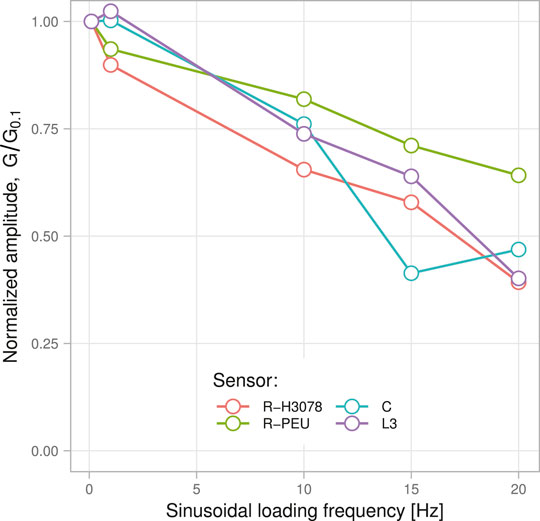
FIGURE 4. Decreasing sensor response under sinusoidal strains of 0.1, 1, 10, 15, and 20 Hz; normalized to the 0.1 Hz trial.

3.3 Signal Hysteresis

Hysteresis is a common nonlinear effect in piezoresistive strain sensors, because the re-aggregation of filler particles and thus formation of conductive pathways may be slow relative to the strain cycles (Stübler et al., 2011). Other sensor types can suffer from mechanical hysteresis of the polymer material that manifests in the signal. A test devised to measure the hysteresis of each sensor type involved straining to six levels with a symmetrical return to zero between each run at a constant strain rate (Supplementary Table S2).

The sensor signal recorded during individual runs are superimposed in Figure 5A. The two resistive sensors showed clockwise signal hysteresis loops, becoming larger in area with less positive slope as the strain maximum was increased. The sensor signal was slightly elevated upon each return to zero for the R-H3078 sensor as well as the R-PEU and C sensors, to a lesser extent. The L3 sensor showed the opposite, with considerable signal undershoot upon return to zero strain.

FIGURE 5

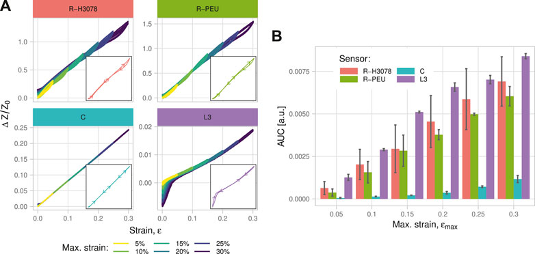
FIGURE 5. Results of the hysteresis test. (A) The overlaid sensor responses to a triangular strain pattern with the directionality of the hysteresis loop at 30% strain shown (inset). (B) Hysteretic loss by sensor type and maximum strain level. Error bars indicate the standard deviation of 3 sequential trials.

One way to compare hysteresis between the sensors is to measure the area encircled by each hysteresis loop (AUC), shown in Figure 5B (Isaia et al., 2020). Multiple loops caused by self-intersection, if present, were summed in absolute area. For a meaningful comparison despite large differences in signal level between sensors, the signal was min-max normalized following Eq. 4.

$\overline{Z}=\frac{Z-Z_0}{Z_{30}-Z_0}(4)$

The C sensor had approximately one seventh the hysteresis area of the R-H3078, R-PEU, or L3 types. Both piezoresistive sensors had similar hysteresis that increased linearly with strain maximum. The R-PEU sensor had greater consistency between runs, especially at higher maximum strains. The L3 sensor showed a linear increase in hysteresis area with strain while the C sensor hysteresis are appeared exponential with respect to strain, albeit having a much lower magnitude. The undershoot at low strains observed with the L3 sensor was the primary contributor to its AUC, with 54% of its total hysteresis AUC attributable to strains below 5%.

3.4 Signal Drift

3.4.1 Static Drift

Rate-dependent hysteresis, material stress relaxation, and temperature changes may contribute to drift of the sensor signal under a constant strain. The test profile (Supplementary Table S3) drove the UTM following a round-trip staircase displacement pattern of up to 30% strain with a hold of 30 s between each step to capture any signal drift. The step profile further allowed the analysis of static drift by comparing the signal drift at different strain levels and approaching those strain levels from lower (extension direction) or higher (recovery direction) preceding strain values.

Static signal drift shown in Figure 6A was found to be influenced by strain magnitude, hold duration—and sometimes—direction of the preceding strain step. The R-H3078 sensor showed monotonic decreases in resistance over time for all cases with the extension direction having less drift than the recovery, although this could be confounded by the ordering of the strain pattern where all extension steps were done prior to all relaxation steps. For the resistive sensors, the $\Delta R/R_0$ drift was mostly independent of strain amount. The drift observed from the R-PEU sensor was similar in magnitude to that of the R-H3078, although with less directionality dependence. The C and L3 sensors showed opposite drifts in signal depending on the directionality of the preceding strain step. Aside from the small change within the first 1 s, the C sensor was very stable and quickly reached steady-state. The L3 sensor had large initial drift, but all trials converged to with 1% of the initial value after 10 s.

FIGURE 6

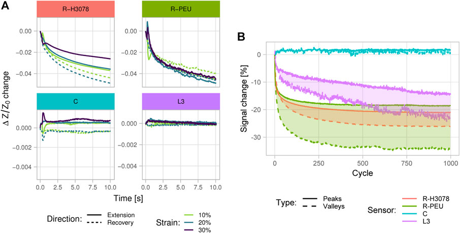
FIGURE 6. Static (A) and dynamic (B) drift in the sensors. (A) Change in sensor signal reading from baseline over a 10 s hold at three strain magnitudes. For increased detail despite a lower sensitivity, the vertical scale of the non-resistive sensors (bottom) is enhanced by a factor of 10. Note that the small transient spike seen around 0.5 s is an artifact that was due to a correction from the UTM positioning algorithm. (B) Sensor signal drift over 1,000 sinusoidal strain cycles. Solid lines indicate the percentage change in signal peaks and dashed lines indicate the percentage change in signal valleys relative to the first cycle.

3.4.2 Dynamic Drift

For reliable tracking over many sessions, a wearable sensor must give a repeatable signal in response to a given strain. The dynamic drift test (Supplementary Table S4) was designed to evaluate sensor resilience and signal drift under cyclic strain. The sensors underwent 1,000 sinusoidal loading cycles from which the initial and final sections may be compared to observe changes in signal amplitude.

As shown in Figure 6B, the piezoresistive sensors had large decreases in response that mostly stabilized within 100 cycles. The L3 sensor had a lower rate of decrease in response but the drift persisted to 1,000 cycles. The C sensor was relatively unaffected by drift, having a small increase in capacitance throughout the first 10 cycles before steady-state response. For all sensor types, the drift behaviour at high and low strains were found to be consistent since the signal peaks and valleys drifted by similar amounts.

3.5 Machine Learning

Regression algorithms were used to predict strain from sensor signals in the presence of nonlinearities. A random UTM displacement signal was produced by generating a random time series normalized such that the points lie in a $\left[\mathrm{0,1}\right]$ range, then scaling and biasing this reference signal for each sensor so that the sample is strained between 5–15%. The reference signal was spline interpolated and low-pass filtered so that the final maximum velocity (strain rate) was $10\mathrm{mm}{\mathrm{s}}^{-1}$ (25%/s). The data collected during the random strain test served as training and test sets for the regression algorithms.

Four regression models plus one model-free scaling approach were compared using 5-fold time series splitting of the random strain data. Training data consisted of the first 10, 20, 30, 40, and 50 s of the data for each fold, respectively, and testing data consisted of the 10 s immediately following the training set. This procedure was chosen over conventional 5-fold cross validation because the SVR, RF, and RNN models (described below) require contiguous past data for training.

A baseline for comparing regression models was a min-max scaling of the sensor signal. Scaling was done so that the signal minimum and maximum were equal to the strain minimum $\left(\epsilon =5\%\right)$ and maximum $\left(\epsilon =15\%\right)$, respectively. The scaling was performed once on the last 50 s of the data set because the dynamic drift effect led to high errors in the initial strain spikes. Fit metrics were computed per fold. The first model considered was a linear regression (LR) completed on each fold. The LR model is essentially the optimal linear scaling that minimizes the mean squared error (MSE) on that fold.

The random forest (RF) and support vector regression (SVR) models are capable of nonlinear regression and were trained over a sliding window of the past 32 sample points or 0.6 s. Parameters were tuned using a coarse grid search followed by ad-hoc fine tuning and were kept the same for all sensors. The RF algorithm had 30 decision trees and the SVR used radial basis functions with $\gamma =0.005$ and $C=0.1$.

The last model of interest was a recurrent neural network (RNN) with 32 recurrent units followed by one fully connected layer, a total of 2,113 parameters. The recurrent units used the rectified linear unit (ReLU) activation function and the dense layer used linear activation. An MSE loss function was used for backpropagation and the recurrent layer had ${\ell }_2$ regularization with a penalty factor of 0.01. The RNN model was also trained with the 32-element sliding window, however, 30% of test data were reserved for validation. The stopping condition for training was a non-decreasing validation MSE over 200 consecutive iterations, typically terminating after 300–700 iterations for the largest fold.

The output of each sensor split by model is shown in Figure 7A. The quality of the regression model fit on the test data for each fold was measured by the R² and root mean squared error (RMSE) with results shown in Figures 7B,C. The results on the first two folds were typically poor because they had a smaller fraction of training data. Average R² and RMSE across the last three folds under the best model for each sensor type compared to that of the scaling model are shown in Table 1, with more detail provided in Supplementary Table S6.

FIGURE 7

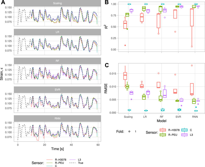
FIGURE 7. Output traces (A) and performance (B), (C) of the regression models trained on random strain data for each sensor type. (A) Strain estimated by each model for each sensor type (solid) and the actual strain (dashed) during the random strain test. (B) Box plots of the coefficient of determination for the four sensors and five regression models. Boxes indicate interquartile range (IQR) and whiskers extend to the smallest and largest observations that are up to 1.5 IQR from the boxes. Outliers are denoted with filled circles while goodness of fit values for the first fold, which often had poor results, are shown with open circles regardless of whether or not they are an outlier. (C) Box plots of the root mean squared error for the four sensors and five regression models.

TABLE 1

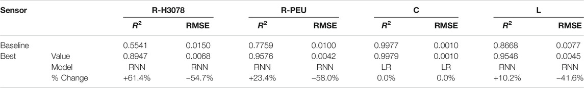
TABLE 1. Improvement in average R² and RMSE across the last three folds by the best performing model for each sensor type.

3.5.1 Effect of the Model on Regression Fit

A Tukey multiple comparison test was run using the results of the last three folds to compare the R² to discriminate models using a given sensor type. For the R-H3078 and R-PEU sensors, only the baseline scaling model had significantly worse R² than all others (p < 0.001). For just the R-H3078 sensor, the SVR model had significantly better R² than LR (p < 0.05), as did the RNN model vs. LR and RF (p < 0.05). For the C sensor, no statistically significant difference between any models was observed. The L3 sensor showed significantly better R² with the SVR model versus scaling, LR, and RF (p < 0.05). A similar pattern of results was produced with respect to RMSE, except with the SVR model no longer having significantly better RMSE over the LR model with the R-H3078 sensor nor over RF with the L3 sensor.

3.5.2 Effect of the Sensor Type on Regression Fit

The same test was run using the R² and RMSE values but using sensors rather than models as factors. The R-H3078 sensor had significantly worse R² than the other sensors across all regression models (p < 0.05), with its best R² and RMSE of 0.8947 and 0.0068, respectively, under the RNN model. The R-PEU sensor had significantly better R² versus the L3 sensor using LR and RF models (p < 0.05). With the RNN model, the R-PEU sensor achieved a best R² value of 0.9576 and RMSE of 0.0042. Regarding RMSE, the R-H3078 sensor again had significantly worse RMSE than the other sensor types under all models (p < 0.025) while the C sensor had significantly better than all the other types (p < 0.005). Like in the R² case, the R-PEU sensor had significantly better RMSE than the L3 sensor using LR and RF (p < 0.025).

4 Discussion

Three fundamentally different fiber strain sensor technologies have been reported previously—piezoresistive, capacitive, and inductive. Each sensor type has characteristics of differing importance when considering the application requirements. The majority of material science research on fiber strain sensors has focused on the increase of sensing range (% strain) and sensitivity (gauge factor). Both of these characteristics are dependent on the composition of the sensor and fabrication methods, important for widening the applications for flexible sensors in motion tracking. In theory, once a flexible sensor is incorporated into a device, the actual performance of the sensor is focused less on the accessible strain range and gauge factor, and more on the signal consistency and the characteristics that are unique to a type of sensor and motion of interest. These characteristics include strain rate and history dependence (hysteresis), gauge factor, linearity, and baseline drift, listed in Table 2 for the sensors tested here. These factors are less prominently explored and can have a large impact on the performance of the sensor in a device beyond the proof-of-concept testing that is typically included in strain sensor reports. If the change of sensor characteristics is predictable, even if not initially obvious, the application of ML prediction models could rectify any perceived limitations and result in a higher tracking accuracy. To begin, three different types of sensors were tested to understand the baseline mechanical properties and identify each characteristic that could be improved with the application of ML. Additionally, two piezoresistive-type sensors (R-H3078 and R-PEU) with different structural core materials were tested to understand the effect of different mechanical properties using this popular type of sensor.

TABLE 2

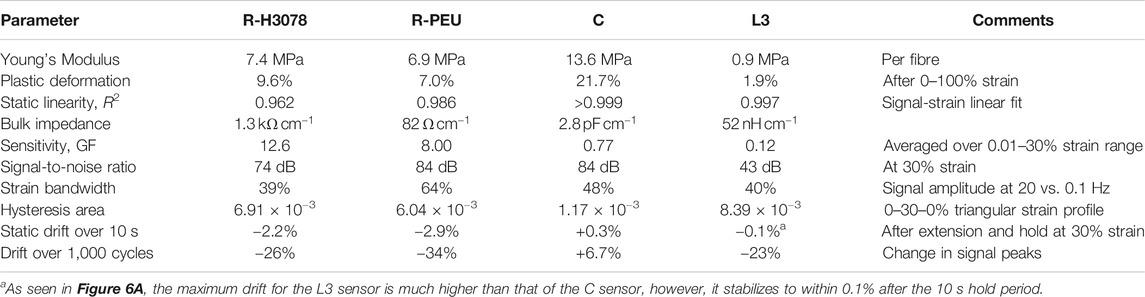
TABLE 2. Summary table for the properties of each sensor studied with any test conditions noted in the comments column.

When tracking mechanical properties during extension, the stress-strain relationship of the polymer sensors (R-H3078, R-PEU, and C) in Figure 3A resembles the gradual decrease in slope with increasing strain reported for TPE-carbon black composites (Drozdov and Dusunceli, 2014). All sensors tested could withstand straining to 100%, indicating that they could tolerate large non-sensing strains which they might be exposed to when donning a garment, for example. The C sensor showed the largest amount of plastic deformation when straining to 100%, although it did not undergo pre-test conditioning which was standard for the other sensors. The L3 sensor was exposed to a lower engineering stress (per-fibre) because the three-loop design had six fibers running in parallel. The mechanical data collected during tensile testing established the elastic region of the sensors which can be useful to limit the amount of irreversible change to the sensors mechanical and electrical characteristics throughout the tests. Using a sensor beyond this region without a highly elastic support can result in a change in signal characteristics, such as gauge factor, by having an irreversible reduction in conductive pathways within the material—which was observed in both piezoresistive sensors. If this irreversible phenomenon occurs in a device that is attempting to track an output, the accuracy of the device post-strain would be impacted. Alternatively, if the irreversible reduction of the conductive pathways is predictable, then machine learning could enable the immediate improvement of device accuracy with enough training data.

Gauge factor is the primary sensor characteristic that relates signal response to strain. A constant, large GF is desirable since it enables linear correlations of signal to strain and increases resolution of small strains across a variety of pre-strains. High resolution is important for tracking fine movements such as facial expressions, where the range of strains is small (Yin et al., 2017). Gauge factors of piezoresistive sensors can vary over three orders of magnitude (Supplementary Table S9); ultimately, most piezoresistive sensors do not possess linear strain-to-resistance changes across both small and large strains. To compare the non-linear response of each sensor, a slow strain rate of 1%/s was used to reduce the possibility of other rate-dependent characteristics impacting the gauge factor results. The increase in GF observed in the R-PEU sensor above 50% strain indicates that the disconnection of conductive pathways becomes the dominant piezoresistive mechanism and may be non-reversible upon release—entrance into this destructive mechanism of piezoresistive sensing is ideally avoided because it results in further negative sensor characteristics for accurate strain tracking such as unrecoverable drift. This motivated the choice to limit further testing to strains below 30% for all sensors. The gauge factor of the R-H3078 sensor peaked at low strain enabling high resolution for small signals. It displays a larger, although more variable, GF across the strain range decreasing from 5–100% strain. The R-PEU shows a more linear working region that persists to a strain of 50%. The nonlinear GF behaviour of both resistive sensors could pose significant negative effects to accuracy tracking. Linearity versus sensitivity is typically an area of trade-off between sensor mechanisms, as shown in Figure 8. The use of ML models to adapt to GF changes in response to certain strain magnitudes or strain rates could then improve the strain tracking accuracy.

FIGURE 8

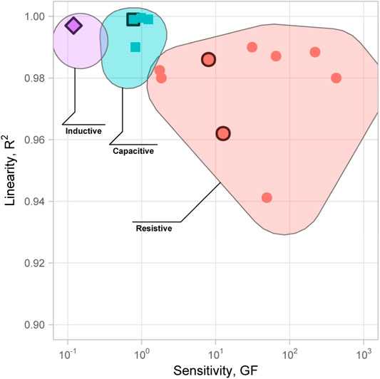
FIGURE 8. The general trade-off between sensitivity, as measured by gauge factor, and linearity, as measured by R² of the linear fit between signal and strain. Clustering between sensor types is suggested by bounding polygons. Examples from literature were chosen that had published GF and R² data (see Supplementary Table S9 for details) and the sensors fabricated in this research are highlighted with a black border.

C and L3 sensors have a lower GF equating to a reduced sensitivity. However, their GF is more constant across the strain range, bringing an increase in accuracy. These types of sensors have a sensing mechanism less dependent on the change of the conductive pathways that may undergo irreversible changes such as in a piezoresistive sensor (Busfield et al., 2003). Increased sensitivity allows the measurement of smaller strain signals using the same readout hardware. While machine learning algorithms may improve sensor accuracy, they offer no improvement to sensitivity. ML models operate after the signal has been digitized and thus are limited by the sensor GF, readout circuit, and ADC in resolving small strains. The reliance on a geometrical change for C and L3 sensors eliminates the negative effects observed in both the piezoresistive sensors and undoubtedly improved the accuracy of C and L3 sensors.

Motion tracking is not always focused on measuring fast, dynamic movements. Some motion tracking devices focus on slight changes in posture over long, nearly static periods. In these situations, signal stability at a static strain over time or between device uses may be more important than sensitivity. Inductive (L3) and piezoresistive (R-PEU/R-H3078) sensors all had signal drift of 3% or greater for 10 s holds at 30% strain, similar to what others have observed for composite sensors (Melnykowycz et al. (2014)). The L3 sensor stabilized during periods of static strain that lasted greater than 10 s, converging to within 1% of its initial value. Its repeatable drift, relatively independent of strain, is a characteristic where ML could impact the signal accuracy. Drift was not observed during the random motion testing for the C and L3 sensors whereas both piezoresistive sensors can be seen to drift following a strain maxima (Figure 7A, Scaling model). Machine learning was able to correct for this drift quite effectively and was observed in the last 5 s of the random motion plots in Figure 7A under the SVR and RNN models. However, the random strain testing patterns were quite short and lacked long static periods that could be used to quantitatively determine how much drift the machine learning compensated for.

Large numbers of repetitive cycles are likely in a lot of applications such as tracking gait parameters. Unsurprising, the C sensor was quite stable, with its reliance on the geometrical change of the fibre, as shown in Figure 6A. Both piezoresistive sensors stabilized after 250 cycles, indicating that sensors required for wearable devices need robust conditioning prior to use. Conditioning could reduce dynamic drift which would decrease the size of the ML training dataset required to predict this type of behaviour. The L3 sensor drifted over the 1,000 cycles at a nearly constant rate, which could allow a simpler ML model to extrapolate the baseline change more easily. The use of simpler models trained with limited data is highly useful for using these devices with ML in actual settings and will be a focus of future research.

The last sensor characteristic that can hinder performance is related to the loading frequency and rate of change of strain. Some applications require the measurement of high frequency strains, such as detecting physiological finger tremors around 6–30 Hz or shank impact shock around 4–40 Hz (Winslow and Shorten, 1989; Raethjen et al., 2000). As loading frequencies are increased, signals can be attenuated by hysteresis (Oliveri et al., 2019; Geng et al., 2020). The effect of high frequency strain on the accuracy and performance of wearable devices using strain sensors has not been extensively explored. A comparison by Shintake et al. that reported a stable signal for both resistive and capacitive sensor types at a maximum tested velocity (strain rate) of $25\mathrm{mm}{\mathrm{s}}^{-1}$ (50%/s) (Shintake et al., 2018). A reduction in the accuracy of the signal could be from either mechanical lag directly correlated to the materials that comprise the sensor, or an effect from the mechanism of sensing (Costa et al., 2015). The comparison of the C and R-H3078 sensors demonstrates that the piezoresistive signal hysteresis is dominant at low loading frequencies because both sensors are comprised of the same materials, but the sensing mechanism of the C sensor eliminates the hysteresis associated with the piezoresistive material by relying on geometrical changes rather than electrode resistivity. As loading frequency increases (Figure 4, the C sensor performance starts to attenuate at a similar rate to the R-H3078 sensor indicating that the mechanical hysteresis phenomenon reduces the tracking performance of both sensors. In contrast, the R-PEU sensor was capable of resolving strain rates up to $126\mathrm{mm}{\mathrm{s}}^{-1}$ with an attenuation of 36%—the best of the sensors tested and can be attributed to the highly elastic and resilient PEU-core (Reza et al., 2019). The R-H3078, C, and L3 sensors had 61%, 52%, and 60% attenuation, respectively. Piezoresistive rubber composites have been shown to measure in excess of $350\mathrm{mm}{\mathrm{s}}^{-1}$ (7000%/s) (Boland et al., 2014). While hysteresis is dependent on the history of the material, ML training with a broad variety of strain patterns and rates could enable the ML to efficiently predict when this phenomenon is causing a reduction in accuracy. Hysteresis was observed in the random strain testing predominantly immediately after large strains followed by faster and smaller strains in Figure 7A. This would be compounded at higher frequencies and could saturate the strain signal leading to a loss of tracking accuracy. Development of high strain bandwidth sensors likely requires more elastic and resilient polymers to reduce any mechanical hysteresis, while ML could be implemented to extend the range of strain frequencies that current sensors can track efficiently.

Each of the characteristics that have been discussed thus far are responsible for the performance of a strain tracking sensor. To gauge the performance of different ML models between different sensing mechanisms, a random strain pattern was generated that had a range representative of what a wearable device for running or walking might produce (Rezaei et al., 2019; Geng et al., 2020; Tavassolian et al., 2020). Different models attempt to predict the applied strain with the resulting signal change—the simplest model being a linear correlation. It was hypothesized that certain combinations of sensors and models may be more accurate when predicting strain by recognizing certain characteristics more efficiently. For instance, sensors with higher degrees of nonlinearity may require a nonlinear regression model (RF, SVR, RNN) to sufficiently correct their signal. The capacitive sensor had an inherently linear response and therefore did not benefit from any ML models. In comparison, the piezoresistive sensors have many characteristics that decrease the accuracy of the strain-signal tracking. The R-PEU linearity was improved by 23% and error reduced by 58% with the RNN model compared to the baseline (scaling) model. Similarly, the same model improved the R-PEU linearity by 61% and reduced fit error by 55% over scaling. The RNN model performed the best, in general, having the highest average R² and lowest average RMSE the context of the random strain experiment. While choosing the best material for the application was shown to be important for applications that require high strain frequencies (specifically elastic and resilient materials such as PEU), ML models have the capability of improving the performance of the devices in the range acceptable similar to optical motion capture devices without the spatial limitations. The advantage of using a combination of R-PEU with a ML model over the C sensor is that the sensor retains its high GF and bandwidth not currently attainable with the capacitive technology. For practical purposes, the simpler analog circuitry needed for resistive sensors and the availability of inexpensive digital computing power to run a model further create scenarios where a piezoresistive sensor would be preferred over the highest performing C sensor. Given the fact that the training dataset used was small and the ability for neural network models to improve with a large amount of data, RNN is a promising model architecture to explore further. The RF model would likely also benefit from a more diverse training dataset because its decision trees were unable to extrapolate accurate predictions outside the training set.

All sensors studied here consist of a single fiber and may be easily incorporated into a garment in areas subject to strain as a linear segment or rectangular patch. Sensors may be anchored to the base textile by means of cross-stitching or encapsulation between layers of fabric. Resistive sensors have the advantage of being read with a simple voltage divider rather than the LC-tank, bridge, or impedance measurement circuit required for the other types. Especially for multichannel systems, resistive sensor arrays with simple interfacing may lead to a significantly reduced number of components and therefore circuit cost. Multichannel systems are common approaches to motion tracking using wearable sensors and the large amount of data collected make such systems a good target for ML improvements. The susceptibility of inductive sensors to noise was observed with the inductive sensor having the lowest SNR in Table 2 and a higher noise floor in Figure 6A. The issue of noise susceptibility with inductive and even un-shielded capacitive sensors have been reported (Yang et al., 2017; Patiño et al., 2020). A summary of qualitative factors relating to the practicality of using each sensor type is shown in Table 3. The acquisition hardware used in this study was limited to a sample rate of 55 Hz making measurements at high strain frequencies unreliable. The method used in Sensor Bandwidth attempts to quantify sensor response to strain rates near the LCR Nyquist frequency, but it would be useful to run a similar experiment with a faster sample rate to confirm the responses to strain rates above 20 Hz. The inclusion of tests to expose the limitations of sensor types that are often not reported combined with the machine learning model results gives insight into which types of limitations may be corrected with modelling, and to what degree, aiding future sensor development.

TABLE 3

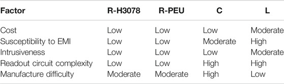
TABLE 3. Ranking of sensors by their relative performance on several qualitative factors.

5 Conclusion

Simpler to manufacture piezoresistive sensors may approach the high degree of strain tracking displayed by capacitive fiber sensors, when combined with machine learning. A piezoresistive sensor is a good candidate for situations with many channels or where high sensitivity is required for tracking fine movements. Piezoresistive sensors also show promise for use with high frequency strain signals, an area that has had relatively little research. Trained nonlinear regression models, such as the SVR and RNN architectures explored here, allow the designer to take advantage of the high sensitivity, bandwidth, ease of manufacturing, and simpler interfacing of piezoresistive sensors by compensating for most of the signal non-idealities. More research is needed into signal conditioning for the inductive sensor types to reduce noise and address the undershoot at low strains, although this technology also benefits from the incorporation of machine learning in its signal processing. Areas of future work may include exploring the direct prediction of joint angle from sensor data with machine learning and expanding the scope of the study to other sensor variants.

Data Availability Statement

The raw data supporting the conclusions of this article will be made available by the authors, without undue reservation.

Author Contributions

CM, TC, and BH contributed to conception and design of the study. BH wrote the first draft of the manuscript. BH and TC wrote sections of the manuscript. All authors contributed to fabrication of the samples, running of the experiments, manuscript revisions, and approval of the submitted manuscript version.

Conflict of Interest

The authors declare that the research was conducted in the absence of any commercial or financial relationships that could be construed as a potential conflict of interest.

Supplementary Material

The Supplementary Material for this article can be found online at: https://www.frontiersin.org/articles/10.3389/fmats.2021.639823/full#supplementary-material.

Footnotes

¹According to the results of an Web of Science topic search conducted October 2020 using the keyword string “wearable sensor” restricted to date range 2009-2019.

References

Boland, C. S., Khan, U., Backes, C., O’Neill, A., McCauley, J., Duane, S., et al. (2014). Sensitive, high-strain, high-rate bodily motion sensors based on graphene-rubber composites. ACS Nano 8, 8819–8830. doi:10.1021/nn503454h

PubMed Abstract | CrossRef Full Text | Google Scholar

Busfield, J. J., Thomas, A. G., and Yamaguchi, K. (2003). Electrical and mechanical behavior of filled elastomers. I: The effect of strain. J. Polym. Sci. Part B Polym. Phys. 41, 2079–2089. doi:10.1002/polb.20085

CrossRef Full Text | Google Scholar

Chen, S., Liu, H., Liu, S., Wang, P., Zeng, S., Sun, L., et al. (2018). Transparent and waterproof ionic liquid-based fibers for highly durable multifunctional sensors and strain-insensitive stretchable conductors. ACS Appl. Mater. Interfaces 10, 4305–4314. doi:10.1021/acsami.7b17790

PubMed Abstract | CrossRef Full Text | Google Scholar

Choi, D. Y., Kim, M. H., Oh, Y. S., Jung, S.-H., Jung, J. H., Sung, H. J., et al. (2017). Highly stretchable, hysteresis-free ionic liquid-based strain sensor for precise human motion monitoring. ACS Appl. Mater. Interfaces 9, 1770–1780. doi:10.1021/acsami.6b12415

PubMed Abstract | CrossRef Full Text | Google Scholar

Clemens, F., Koll, B., Graule, T., Watras, T., Binkowski, M., Mattmann, C., et al. (2012). Development of piezoresistive fiber sensors, based on carbon black filled thermoplastic elastomer compounds, for textile application. Adv. Sci. Technol. 80, 7–13. doi:10.4028/www.scientific.net/ast.80.7

CrossRef Full Text | Google Scholar

Cooper, C. B., Arutselvan, K., Liu, Y., Armstrong, D., Lin, Y., Khan, M. R., et al. (2017). Stretchable capacitive sensors of torsion, strain, and touch using double helix liquid metal fibers. Adv. Funct. Mater. 27, 1605630. doi:10.1002/adfm.201605630

CrossRef Full Text | Google Scholar

Costa, P., Ribeiro, S., and Lanceros-Mendez, S. (2015). Mechanical vs. electrical hysteresis of carbon nanotube/styrene-butadiene-styrene composites and their influence in the electromechanical response. Compos. Sci. Technol. 109, 1–5. doi:10.1016/j.compscitech.2015.01.006

CrossRef Full Text | Google Scholar

De Focatiis, D. S. A., Hull, D., and Sánchez-Valencia, A. (2012). Roles of prestrain and hysteresis on piezoresistance in conductive elastomers for strain sensor applications. Plast. Rubber Compos. 41, 301–309. doi:10.1179/1743289812Y.0000000022

CrossRef Full Text | Google Scholar

Diani, J., Fayolle, B., and Gilormini, P. (2009). A review on the Mullins effect. Eur. Polym. J. 45, 601–612. doi:10.1016/j.eurpolymj.2008.11.017

CrossRef Full Text | Google Scholar

Drozdov, A. D., and Dusunceli, N. (2014). Unusual mechanical response of carbon black-filled thermoplastic elastomers. Mech. Mater. 69, 116–131. doi:10.1016/j.mechmat.2013.09.019

CrossRef Full Text | Google Scholar

Fleury, A., Sugar, M., and Chau, T. (2015). E-textiles in clinical rehabilitation: a scoping review. Electronics 4, 173–203. doi:10.3390/electronics4010173

CrossRef Full Text | Google Scholar

Frutiger, A., Muth, J. T., Vogt, D. M., Mengüç, Y., Campo, A., Valentine, A. D., et al. (2015). Capacitive soft strain sensors via multicore-shell fiber printing. Adv. Mater. 27, 2440–2446. doi:10.1002/adma.201500072

PubMed Abstract | CrossRef Full Text | Google Scholar

Geng, W., Cuthbert, T. J., and Menon, C. (2020). Conductive thermoplastic elastomer composite capacitive strain sensors and their application in a wearable device for quantitative joint angle prediction. ACS Appl. Polym. Mater. 3, 122–129. doi:10.1021/acsapm.0c00708

CrossRef Full Text | Google Scholar

He, Z., Zhou, G., Byun, J-H., Lee, S-K., Um, M-K., Park, B., et al. (2019). Highly stretchable multi-walled carbon nanotube/thermoplastic polyurethane composite fibers for ultrasensitive, wearable strain sensors. Nanoscale 11, 5884–5890. doi:10.1039/C9NR01005J

PubMed Abstract | CrossRef Full Text | Google Scholar

Isaia, C., McMaster, S. A., and McNally, D. (2020). “Study of performance of knitted conductive sleeves as wearable textile strain sensors for joint motion tracking,” in 42nd annual international conference of the IEEE engineering in medicine & biology society (EMBC), Montreal, QC, July 20–24, 2020 (IEEE), 4555–4558.

Google Scholar

Jung, Y., Jung, K., Park, B., Choi, J., Kim, D., Park, J., et al. (2019). Wearable piezoresistive strain sensor based on graphene-coated three-dimensional micro-porous PDMS sponge. Micro Nano Syst. Lett. 7, 1–9. doi:10.1186/s40486-019-0097-2

CrossRef Full Text | Google Scholar

Kalantari, M., Dargahi, J., Kövecses, J., Mardasi, M. G., and Nouri, S. (2012). A new approach for modeling piezoresistive force sensors based on semiconductive polymer composites. IEEE/ASME Trans. Mechatron. 17, 572–581. doi:10.1109/TMECH.2011.2108664

CrossRef Full Text | Google Scholar

Keulemans, G., Ceyssens, F., and Puers, R. (2017). An ionic liquid based strain sensor for large displacement measurement. Biomed. Microdevices 19, 1123–1126. doi:10.1007/s10544-016-0141-4

CrossRef Full Text | Google Scholar

Kim, J-S., and Kim, G-W. (2017). Hysteresis compensation of piezoresistive carbon nanotube/polydimethylsiloxane composite-based force sensors. Sensors 17, 229–241. doi:10.3390/s17020229

CrossRef Full Text | Google Scholar

Kim, S-R., Kim, J-H., and Park, J-W. (2017). Wearable and transparent capacitive strain sensor with high sensitivity based on patterned Ag nanowire networks. ACS Appl. Mater. Interfaces 9, 26407–26416. doi:10.1021/acsami.7b06474

PubMed Abstract | CrossRef Full Text | Google Scholar

Laskoski, G. T., Martins, L. D. L., Pichorim, S. F., and Abatti, P. J. (2009). “Development of a telemetric goniometer,” in World congress on medical physics and biomedical engineering, Munich, Germany, September 7–12, 2009 (Berlin, Germany: Springer), 227–230.

CrossRef Full Text | Google Scholar

Lee, J., Kwon, H., Seo, J., Shin, S., Koo, J. H., Pang, C., et al. (2015). Conductive fiber-based ultrasensitive textile pressure sensor for wearable electronics. Adv. Mater. 27, 2433–2439. doi:10.1002/adma.201500009

PubMed Abstract | CrossRef Full Text | Google Scholar

Liu, N., Fang, G., Wan, J., Zhou, H., Long, H., and Zhao, X. (2011). Electrospun PEDOT:PSS-PVA nanofiber based ultrahigh-strain sensors with controllable electrical conductivity. J. Mater. Chem. 21, 18962–18966. doi:10.1039/c1jm14491j

CrossRef Full Text | Google Scholar

Liu, Z. F., Fang, S., Moura, F. A., Ding, J. N., Jiang, N., Di, J., et al. (2015). Hierarchically buckled sheath-core fibers for superelastic electronics, sensors, and muscles. Science 349, 400–404. doi:10.1126/science.aaa7952

PubMed Abstract | CrossRef Full Text | Google Scholar

Liu, Y., Wang, H., Zhao, W., Zhang, M., Qin, H., and Xie, Y. (2018a). Flexible, stretchable sensors for wearable health monitoring: sensing mechanisms, materials, fabrication strategies and features. Sensors 18, 645–680. doi:10.3390/s18020645

CrossRef Full Text | Google Scholar

Liu, Y. F., Li, Y. Q., Huang, P., Hu, N., and Fu, S. Y. (2018b). On the evaluation of the sensitivity coefficient of strain sensors. Adv. Electron. Mater. 4, 1800353. doi:10.1002/aelm.201800353

CrossRef Full Text | Google Scholar

Mengüç, Y., Park, Y.-L., Pei, H., Vogt, D., Aubin, P. M., Winchell, E., et al. (2014). Wearable soft sensing suit for human gait measurement. Int. J. Rob. Res. 33, 1748–1764. doi:10.1177/0278364914543793

CrossRef Full Text | Google Scholar

Michel, S., Chu, B. T. T., Grimm, S., Nüesch, F. A., Borgschulte, A., and Opris, D. M. (2012). Self-healing electrodes for dielectric elastomer actuators. J. Mater. Chem. 22, 20736–20741. doi:10.1039/c2jm32228e

CrossRef Full Text | Google Scholar

Miodownik, M., Oldfrey, B., Jackson, R., and Smitham, P. (2019). A deep learning approach to non-linearity in wearable stretch sensors. Front. Robot. AI 6, 27. doi:10.3389/frobt.2019.00027

PubMed Abstract | CrossRef Full Text | Google Scholar

Oliveri, A., Maselli, M., Lodi, M., Storace, M., and Cianchetti, M. (2019). Model-based compensation of rate-dependent hysteresis in a piezoresistive strain sensor. IEEE Trans. Ind. Electron. 66, 8205–8213. doi:10.1109/TIE.2018.2884204

CrossRef Full Text | Google Scholar

Patiño, A. G., Khoshnam, M., and Menon, C. (2020). Wearable device to monitor back movements using an inductive textile sensor. Sensors 20, 905–922. doi:10.3390/s20030905

CrossRef Full Text | Google Scholar

Patron, D., Mongan, W., Kurzweg, T. P., Fontecchio, A., Dion, G., Anday, E. K., et al. (2016). On the use of knitted antennas and inductively coupled RFID tags for wearable applications. IEEE Trans. Biomed. Circuits Syst. 10, 1047–1057. doi:10.1109/TBCAS.2016.2518871

PubMed Abstract | CrossRef Full Text | Google Scholar

Raethjen, J., Pawlas, F., Lindemann, M., Wenzelburger, R., and Deuschl, G. (2000). Determinants of physiologic tremor in a large normal population. Clin. Neurophysiol. 111, 1825–1837. doi:10.1016/S1388-2457(00)00384-9

PubMed Abstract | CrossRef Full Text | Google Scholar

Reza, M. S., Ayag, K. R., Yoo, M. K., Kim, K. J., and Kim, H. (2019). Electrospun spandex nanofiber webs with ionic liquid for highly sensitive, low hysteresis piezocapacitive sensor. Fibers Polym. 20, 337–347. doi:10.1007/s12221-019-8778-2

CrossRef Full Text | Google Scholar

Rezaei, A., Cuthbert, T. J., Gholami, M., and Menon, C. (2019). Application-based production and testing of a core-sheath fiber strain sensor for wearable electronics: feasibility study of using the sensors in measuring tri-axial trunk motion angles. Sensors 19, 4288–4313. doi:10.3390/s19194288

CrossRef Full Text | Google Scholar

Sardini, E., Serpelloni, M., and Ometto, M. (2012). “Smart vest for posture monitoring in rehabilitation exercises,” in Proceedings of 2012 IEEE sensors applications symposium, SAS 2012 - proceedings, Brescia, Italy, February 7–9, 2012 (IEEE), 161–165.

Google Scholar

Seyedin, S., Razal, J. M., Innis, P. C., Jeiranikhameneh, A., Beirne, S., and Wallace, G. G. (2015). Knitted strain sensor textiles of highly conductive all-polymeric fibers. ACS Appl. Mater. Interfaces 7, 21150–21158. doi:10.1021/acsami.5b04892

PubMed Abstract | CrossRef Full Text | Google Scholar

Shin, M. K., Oh, J., Lima, M., Kozlov, M. E., Kim, S. J., and Baughman, R. H. (2010). Elastomeric conductive composites based on carbon nanotube forests. Adv. Mater. 22, 2663–2667. doi:10.1002/adma.200904270

PubMed Abstract | CrossRef Full Text | Google Scholar

Shintake, J., Piskarev, E., Jeong, S. H., and Floreano, D. (2018). Ultrastretchable strain sensors using carbon black-filled elastomer composites and comparison of capacitive versus resistive sensors. Adv. Mater. Technol. 3, 1700284. doi:10.1002/admt.201700284

CrossRef Full Text | Google Scholar

Stübler, N., Fritzsche, J., and Klüppel, M. (2011). Mechanical and electrical analysis of carbon black networking in elastomers under strain. Polym. Eng. Sci. 51, 1206–1217. doi:10.1002/pen.21888

CrossRef Full Text | Google Scholar

Tavassolian, M., Cuthbert, T. J., Napier, C., Peng, J., and Menon, C. (2020). Textile‐based inductive soft strain sensors for fast frequency movement and their application in wearable devices measuring multiaxial hip joint angles during running. Adv. Intell. Syst. 2, 1900165. doi:10.1002/aisy.201900165

CrossRef Full Text | Google Scholar

Vu, C. C., and Kim, J. (2018). Human motion recognition by textile sensors based on machine learning algorithms. Sensors 18, 3109–3125. doi:10.3390/s18093109

CrossRef Full Text | Google Scholar

Wang, H., Liu, Z., Ding, J., Lepró, X., Fang, S., Jiang, N., et al. (2016). Downsized sheath-core conducting fibers for weavable superelastic wires, biosensors, supercapacitors, and strain sensors. Adv. Mater. 28, 4998–5007. doi:10.1002/adma.201600405

PubMed Abstract | CrossRef Full Text | Google Scholar

Wijesiriwardana, R. (2006). Inductive fiber-meshed strain and displacement transducers for respiratory measuring systems and motion capturing systems. IEEE Sens. J. 6, 571–579. doi:10.1109/JSEN.2006.874488

CrossRef Full Text | Google Scholar

Winslow, D. S., and Shorten, M. R. (1989). Spectral analysis of impact shock during running. J. Appl. Biomech. 8, 288–304. doi:10.1016/0021-9290(89)90511-3

CrossRef Full Text | Google Scholar

Wu, X., Han, Y., Zhang, X., and Lu, C. (2016). Highly sensitive, stretchable, and wash-durable strain sensor based on ultrathin conductive Layer@Polyurethane yarn for tiny motion monitoring. ACS Appl. Mater. Interfaces 8, 9936–9945. doi:10.1021/acsami.6b01174

PubMed Abstract | CrossRef Full Text | Google Scholar

Yang, T., Xie, D., Li, Z., and Zhu, H. (2017). Recent advances in wearable tactile sensors: materials, sensing mechanisms, and device performance. Mater. Sci. Eng. R Rep. 115, 1–37. doi:10.1016/j.mser.2017.02.001

CrossRef Full Text | Google Scholar

Yin, B., Wen, Y., Hong, T., Xie, Z., Yuan, G., Ji, Q., et al. (2017). Highly stretchable, ultrasensitive, and wearable strain sensors based on facilely prepared reduced graphene oxide woven fabrics in an ethanol flame. ACS Appl. Mater. Interfaces 9, 32054–32064. doi:10.1021/acsami.7b09652

PubMed Abstract | CrossRef Full Text | Google Scholar

Jia, F., Li, X., Peng, H., Li, F., Yang, K., and Yuan, W. (2019). A highly sensitive, multifunctional, and wearable mechanical sensor based on RGO/synergetic fiber bundles for monitoring human actions and physiological signals. Sens. Actuators B 285, 179–185. doi:10.1016/j.snb.2019.01.063

CrossRef Full Text | Google Scholar

Zahid, M., Papadopoulou, E. L., Athanassiou, A., and Bayer, I. S. (2017). Strain-responsive mercerized conductive cotton fabrics based on PEDOT:PSS/graphene. Mater. Des. 135, 213–222. doi:10.1016/j.matdes.2017.09.026

CrossRef Full Text | Google Scholar

Zhang, Z., Zheng, J., Wu, H., Wang, W., Wang, B., and Liu, H. (2012). Development of a respiratory inductive plethysmography module supporting multiple sensors for wearable systems. Sensors 12, 13167–13184. doi:10.3390/s121013167

PubMed Abstract | CrossRef Full Text | Google Scholar

Zheng, S., Wu, X., Huang, Y., Xu, Z., Yang, W., Liu, Z., et al. (2019). Highly sensitive and multifunctional piezoresistive sensor based on polyaniline foam for wearable Human-Activity monitoring. Composites Part A 121, 510–516. doi:10.1016/j.compositesa.2019.04.014

CrossRef Full Text | Google Scholar