Large-Scale Statistical Learning for Mass Transport Prediction in Porous Materials Using 90,000 Artificially Generated Microstructures

1 Introduction

The performance of functional materials is significantly influenced by the underlying 3D structure and morphology (Torquato, 2002; Willot and Forest, 2018). Thus, optimizing 3D microstructures for high performance in particular applications is one of the main goals in many branches of materials research. Typically, the amount of candidate materials structures is enormous and beyond the reach of conventional experimental screening (Dunn et al., 2020; Saunders et al., 2021) (for example, the number of potential pharmacologically active molecules is at least 10²⁰ and theoretically estimated at 10⁶⁰) (Hoffmann and Gastreich, 2019). To overcome this limitation, virtual materials testing is an approach of increasing importance, where mathematical models are used for both the analysis of artificially generated materials structures, as well as for the investigation of their effective properties. By systematically varying the model parameters, a large number of virtual but realistic 3D microstructures can be drawn from stochastic models just at the cost of computer simulations. These structures serve as geometry input for spatially-resolved numerical simulations of effective properties. In this way, together with the computation of various descriptors of the 3D microstructures, quantitative microstructure-property relationships can be established.

Typically, the mathematical models of random porous microstructures with two phases, solid and pores, are located in the (continuous) Euclidean space. If we restrict ourselves to discrete representations on a computational grid, say a cube of N³ lattice points, the number of theoretically possible structures is $2^{N^3}$. Although many of those structures are not suitable to describe real materials, still a huge number of structural scenarios remains for which this is the case. In virtual materials testing, 3D microstructures are typically explored by means of parametric models that span some region of interest, using tools from mathematical morphology and stochastic geometry (Lantuéjoul, 2002; Chiu et al., 2013; Jeulin, 2021). These microstructure models can be calibrated with experimental data gained, e.g., by tomographic imaging or simply be inspired by experimentally observed structures. There are numerous examples for artificial generation and virtual testing of functional materials, including applications for lithium ion batteries (Feinauer et al., 2015; Hein et al., 2016; Westhoff et al., 2018a; Prifling et al., 2019; Hein et al., 2020; Allen et al., 2021; Prifling et al., 2021a; Birkholz et al., 2021; Furat et al., 2021), solid oxide fuel cells (Abdallah et al., 2016; Neumann et al., 2016; Moussaoui et al., 2018), amorphous silica (Prifling et al., 2021b), gas diffusion electrodes (Neumann et al., 2019a), open-cell foams (Westhoff et al., 2018b), organic semiconductors (Westhoff et al., 2015), mesoporous alumina (Wang et al., 2015), solar cells (Stenzel et al., 2011), electric double-layer capacitors (Prill et al., 2017), platelet-filled composites (Röding et al., 2018), fiber-based materials (Röding et al., 2016; Townsend et al., 2021), and pharmaceutical coatings for controlled drug release (Barman et al., 2019).

The focus of the present paper is on quantifying the influence of 3D microstructure on mass transport properties of porous materials and, specifically, in effective diffusivity and fluid permeability. There are numerous microstructural descriptors that are useful for the prediction of those properties. The most fundamental one is porosity, followed by specific surface area i.e., the pore-solid interface area per unit volume. However, there are many more sophisticated structural descriptors considered in literature, e.g., various measures of tortuosity, pore size distributions, constrictivity, and two-point correlation functions. Various combinations of such descriptors have been used to establish microstructure-property relationships of varying complexity. The most well-known relationship for permeability is perhaps the Kozeny-Carman equation which in its basic form only uses porosity and specific surface area to describe the underlying 3D microstructure (Kozeny, 1927; Carman, 1937). For effective diffusivity, there exist equally simple formulas, in some cases involving only porosity (Masaro and Zhu, 1999). Later on, analytical expressions of this type have been developed where more complex structural descriptors have been taken into account, such as constrictivity and tortuosity (Barman et al., 2019; Neumann. et al., 2020), as well as two-point correlation functions (Berryman, 1985; Torquato, 1991; Jiao and Torquato, 2012; Liasneuski et al., 2014; Hlushkou et al., 2015; Ma and Torquato, 2018). Some of these formulas still are sufficiently simple to allow a certain physical interpretation. On the other hand, numerous attempts have been made to use high-dimensional regression methods and machine learning in order to obtain more accurate prediction models, where the descriptors of 3D microstructures and mass transport properties, as input and output variables, still have physical underpinnings. But the relationships derived between them are, in a sense, more data-driven and less determined by the underlying physics, where this effect amplifies with increasing dimension and complexity of the prediction model. For example, in van der Linden et al. (2016), the permeability and 27 different microstructural descriptors were computed for 536 granular materials structures. This information was then used to develop (log-)linear relationships and find relevant subsets of descriptors through variable selection procedures. In Stenzel et al. (2017), effective conductivity (mathematically equivalent to effective diffusivity) and numerous structural descriptors including constrictivity and tortuosity were computed for 8,119 microstructures, where conventional regression, random forests, and artificial neural networks (ANNs) were used for prediction. In Röding et al. (2020), permeability, tortuosity and two-point correlation functions were computed for 30,000 structures, where log-linear regression and ANNs were used for prediction. Although machine learning regression using ANNs is less transparent compared to analytical prediction formulas and hence less interpretable, the benefit of this approach is that arbitrarily complex relationships can be represented by a feed-forward network due to the universal approximation theorem (Cybenko, 1989; Hornik et al., 1989). Hence, machine learning regression can be considered a data-science approach that leads to insight into new relationships and into which descriptors are most useful for prediction (Umehara et al., 2019; Röding et al., 2020). A third option is the prediction of effective properties using convolutional neural networks (CNNs). Note that conventional ANNs learn to perform nonlinear regression using predefined descriptors, whereas CNNs perform their own descriptor extraction directly from the microstructure, expressed as nonlinear compositions of convolution filters. These are then used as input to a conventional ANN that performs the regression (Kawaguchi et al., 2021). CNNs have been used for predicting both permeability (Srisutthiyakorn, 2016; Wu et al., 2018; Araya-Polo et al., 2019; Sudakov et al., 2019; Graczyk and Matyka, 2020; Kamrava et al., 2020) and effective diffusivity (Wu et al., 2019; Wang et al., 2020), although in many cases with small datasets and/or only with 2D structures. Generally, CNNs have the tendency to be even less transparent than ANNs in terms of understanding how the prediction works.

In the present paper, we investigate an extremely broad range of virtual two-phase microstructures which are drawn from nine different stochastic models. For each model type, 10,000 microstructures are generated for different specifications of model parameters leading, e.g., to varying porosities and length scales. Hence, in total, our study comprises 90,000 microstructures. For each structure, both effective diffusivity and permeability are computed. Furthermore, a multitude of structural descriptors is determined, like porosity, specific surface area, median pore radius, radius of the characteristic bottleneck, constrictivity, tortuosity (and its distribution), chord lengths (and their distribution), spherical contact distribution, and two-point correlation functions. The dimension of the largest possible descriptor space is equal to 236. As already mentioned above, we utilize analytical prediction formulas as well as ANNs and CNNs to establish microstructure-property relationships. Due to the large diversity of the dataset considered in this paper, the determined relationships are not specific to any particular morphology, but rather quite generally applicable. For CNNs, in particular, large amounts of data are needed to ensure robust training and good generalization to new data. Thus, to the best of our knowledge, the data considered in this paper is the largest and most diverse dataset for the study of effective diffusivity and permeability, which has been reported so far in the literature. To facilitate further development of microstructure-property relationships and their predictive power, the microstructures, their corresponding morphological and effective properties, and the code used to study microstructure-property relationships are available open access (Prifling et al., 2021c). Note that besides the comprehensive database for porous materials considered in the present paper, there are several further research activities of this kind for other types of materials, e.g., for composite particulate materials occurring in crushed ores (Ditscherlein et al., 2021).

The rest of this paper is organized as follows. In Section 2 the definitions of various structural descriptors are explained as well as their estimation from 3D image data. They are used as input variables for establishing microstructure-property relationships. Then, in Section 3, two descriptors of effective properties, namely diffusivity and permeability of the pore space, are presented, which serve as output variables. Section 4 introduces the stochastic models used for the artificial generation of 3D microstructures, whereas in Section 5 three different approaches are explained which are applied to establish the microstructure-property relationships. Finally, a discussion of the results obtained in this paper is provided in Section 6.

2 Structural Descriptors and Their Estimation

The goal of this section is to explain the definitions of various structural descriptors considered in this paper as well as methods for their estimation from simulated 3D image data, where the underlying stochastic 3D microstructure models described in Section 4 are stationary and isotropic. This implies that the pore space is a stationary and isotropic random set as well, which will be denoted by Ξ in the following, i.e., its distribution is invariant with respect to translations of and rotations around the origin (Lantuéjoul, 2002; Chiu et al., 2013; Jeulin, 2021). Note that all microstructures that are drawn from these stochastic models fulfill periodic boundary conditions in x-, y- and z-directions. This is taken into account when estimating the structural descriptors as presented below. In addition to simple scalar descriptors of Ξ such as volume fraction, specific surface area or constrictivity, we also consider more complex descriptors like the chord length distribution, the spherical contact distribution and the distribution of geodesic tortuosity. In practice, we represent these distributions by their quantiles, starting from 5%- up to 95%-quantiles in 5% steps.

2.1 Porosity

To begin with, we consider one of the simplest but most important structural descriptors, namely the porosity ɛ ∈ [0, 1], i.e., the volume fraction of the random pore space $\mathrm{\Xi }\subset {\mathbb{R}}^3$, where $\epsilon =\mathbb{E}({\nu }_3(\mathrm{\Xi }\cap {[\mathrm{0,1}]}^3))$ and ν₃ denotes the three-dimensional Lebesgue measure. This characteristic can be easily estimated from 3D image data by the point-count method (Chiu et al., 2013). Note that this estimation method has obviously not to be adapted further to account for periodic boundary conditions.

2.2 Specific Surface Area

A further relevant scalar descriptor is the specific surface area of the interface between solid and pores, denoted by S > 0. It is defined as the expected surface area of the pore space per unit volume. In order to estimate this characteristic from voxelized binary images, we compute weighted sums by considering local 2 × 2 × 2 voxel configurations, where we use the weights proposed by Schladitz et al. (2007). Periodic boundary conditions are taken into account by a circular padding of size one in each direction using the Matlab command “padarray” (MATLAB, 2021).

2.3 Geodesic Tortuosity

Next, we consider the geodesic tortuosity of the pore space, which is a purely geometric quantity that significantly influences effective properties (Stenzel et al., 2016; Barman et al., 2019; Neumann. et al., 2020; Holzer et al., 2021). It is important to point out that different concepts of tortuosity exist in the literature (Clennell, 1997; Ghanbarian et al., 2013; Tjaden et al., 2018). The general idea is to consider shortest paths from a predefined starting plane to a target plane, which have to be completely contained in the pore phase. This means, that we consider the shortest path with respect to the geodesic metric of the pore space (Lantuéjoul and Maisonneuve, 1984). Then, the distribution of the lengths τ_geo of those shortest paths, divided by the distance of the two planes, is denoted by d(τ_geo). Recall that, in this paper, the distribution d(τ_geo) is represented by 19 quantiles, starting from 5%- up to 95%-quantiles in 5% steps. Furthermore, mean geodesic tortuosity, denoted by m(τ_geo) ≥ 1, is defined as the mean value of the random variable τ_geo, whereas its standard deviation is denoted by σ(τ_geo). A more formal definition of these quantities within the framework of random sets can be found in Neumann et al. (2019b), whereas a slightly different definition of geodesic tortuosity is presented in Barman et al. (2019). Regarding the estimation of the distribution of geodesic tortuosity from 3D image data, we compute the shortest paths with the Dijkstra algorithm (Jungnickel, 2007), where the transport direction is from low x-values to high x-values. Note that the transport paths are allowed to “leave” the sampling window in the y- and z-directions in order to account for periodic boundary conditions.

2.4 Constrictivity

In order to define the constrictivity of the pore space, denoted by β ∈ [0, 1], we first describe the continuous pore size distribution (CPSD) as well as the concept of simulated mercury intrusion porosimetry (MIP). The continuous pore size distribution $\mathrm{C}\mathrm{P}\mathrm{S}\mathrm{D}:[0,\infty )\to [\mathrm{0,1}]$ has been introduced in Münch and Holzer (2008) and is based on a morphological opening (Serra, 1982; Soille, 2003). More precisely, for each radius r ≥ 0, the value $\mathrm{C}\mathrm{P}\mathrm{S}\mathrm{D}(r)$ is given by the volume fraction of the pore space that can be covered by a potentially overlapping union of spheres with radius r, which have to be completely contained in the pore space. The radius r_max is now defined as the radius for which $\mathrm{C}\mathrm{P}\mathrm{S}\mathrm{D}(r_{\text{max}})$ equals half of the porosity, i.e., $\mathrm{C}\mathrm{P}\mathrm{S}\mathrm{D}(r_{\text{max}})=\mathrm{C}\mathrm{P}\mathrm{S}\mathrm{D}(0)/2$. The estimation of $\mathrm{C}\mathrm{P}\mathrm{S}\mathrm{D}(r)$ from image data relies on the computation of the so-called Euclidean distance transform (Maurer et al., 2003; Soille, 2003), which allows to perform an erosion followed by a dilation using a ball with radius r as structuring element. In order to take periodic boundary conditions into account, the computation of the Euclidean distance transform has to be adapted as follows. At first, a circular padding is applied to the binary image leading to a 3D image, which is twice as large in each of the three directions. In a second step, the Euclidean distance transform is computed on the enlarged image. Afterwards, a 3D cutout with the same size as the original image, whose centroid corresponds to the centroid of the enlarged Euclidean distance transform, is cut out of the enlarged Euclidean distance transform. Finally, a circular shift is applied to this cutout using the “circshift” command in Matlab in order to restore the original spatial arrangement of the voxels (MATLAB, 2021).

The concept of simulated mercury intrusion porosimetry (MIP) is similar to that of the CPSD, except that MIP depends in general on a predefined direction. More precisely, the union of potentially overlapping balls of radius r considered above has to form an intrusion from the given direction, when computing the correspondingly modified volume fraction $\mathsf{M}\mathsf{I}\mathsf{P}(r)$. This accounts for bottlenecks in the pore space such that the values of the function $\mathrm{M}\mathrm{I}\mathrm{P}:[0,\infty )\to [\mathrm{0,1}]$ are always less or equal than the corresponding values of $\mathrm{C}\mathrm{P}\mathrm{S}\mathrm{D}:[0,\infty )\to [\mathrm{0,1}]$, i.e., $\mathrm{M}\mathrm{I}\mathrm{P}(r)\le \mathrm{C}\mathrm{P}\mathrm{S}\mathrm{D}(r)$ for all r ≥ 0. In order to simulate the intrusion from low x-values to high x-values, the Hoshen-Kopelman algorithm is used (Hoshen and Kopelman, 1976), where it is straightforward to apply periodic boundary conditions in y- and z-directions. Note that due to our stationarity and isotropy assumptions, the values of $\mathsf{M}\mathsf{I}\mathsf{P}$ do not depend on the choice of the predefined direction. However, within the present paper, this quantity is computed in x-direction, where the intrusion starts at low x-values. Analogously to r_max, the radius r_min is defined as the radius for which $\mathrm{M}\mathrm{I}\mathrm{P}(r_{\text{min}})$ equals half the porosity, i.e., $\mathrm{M}\mathrm{I}\mathrm{P}(r_{\text{min}})=\mathrm{C}\mathrm{P}\mathrm{S}\mathrm{D}(0)/2$.

The constrictivity of the pore space is now given by $\beta ={(\frac{r_{\text{min}}}{r_{\text{max}}})}^2\in [\mathrm{0,1}]$ (Münch and Holzer, 2008), where a constrictivity of one occurs if there are no constrictions within the pore space at all. The lower the constrictivity, the more the transport within the pore space is hindered by bottlenecks. This geometric characteristic has turned out to significantly influence effective properties of functional materials (Holzer et al., 2013). A formal definition of constrictivity within the framework of random sets can be found in Neumann et al. (2019b).

2.5 Chord Length Distribution

The chord length distribution of the pore space, which is modelled by a stationary random set $\mathrm{\Xi }\subset {\mathbb{R}}^3$, is defined as follows (Ohser and Mücklich, 2000; Ohser and Schladitz, 2009; Chiu et al., 2013). Given a predefined direction $\phi \in [0,\frac{\pi }{2}]\times [\mathrm{0,2}\pi )$, the chord length distribution of the random set Ξ in direction φ is the distribution of the length L of the so-called typical line segment (selected at random) in Ξ ∩ ℓ, where ℓ denotes the line passing through the origin in direction φ. The distribution of L is denoted by d(L) and, again, represented by 19 quantiles, starting from 5%- up to 95%-quantiles in 5% steps. Note that d(L) does not depend on the particular choice of φ, when considering stationary and isotropic random sets. The mean and the standard deviation of the chord length distribution are denoted by m(L) and σ(L), respectively. In the present paper, observing Ξ ∩ ℓ ∩ W within some sampling window $W\subset {\mathbb{R}}^3$, the chord length distribution is estimated by counting subsequent voxels belonging to the pore space along the x-axis and computing the empirical distribution function of the lengths of these voxel sequences. Note that periodic boundary conditions can be simply accounted for by merging the first and the last chord in Ξ ∩ ℓ ∩ W, provided that both chords belong to the pore space.

2.6 Spherical Contact Distribution

Consider the (random) distance H from the typical point of ${\mathrm{\Xi }}^c={\mathbb{R}}^3\backslash \mathrm{\Xi }$ to the nearest point within Ξ. The function F_H: [0, ∞) → [0, 1] with $F_H(r)=\mathbb{P}(H\le r)$ for each r ≥ 0 is called the spherical contact distribution function of Ξ. Note that the values of F_H are given by

$F_H(r)=1-\frac{\mathbb{P}(\mathrm{\Xi }\cap B(o,r)=\varnothing )}{1-\epsilon }\text{for\hspace{0.17em}each\hspace{0.17em}}r\ge 0,$

where $B(o,r)\subset {\mathbb{R}}^3$ denotes the closed ball with radius r centered at the origin (Chiu et al., 2013). The mean, standard deviation and distribution of H are denoted by m(H), σ(H) and d(H), respectively. These quantities can be estimated from voxelized 3D image data using the algorithm proposed by Mayer (2004), which relies on the computation of the Euclidean distance transform. Thus, periodic boundary conditions are taken into account by computing the Euclidean distance transform with respect to periodic boundary conditions as described above in Section 2.4. As in case of the distribution of geodesic tortuosity and the chord length distribution, the distribution d(H) is represented by 19 quantiles.

2.7 Two-Point Correlation Function

For a stationary and isotropic random set $\mathrm{\Xi }\subset {\mathbb{R}}^3$ describing the pore space of a porous material, the two-point (pore-pore) correlation function C: [0, ∞) → [0, 1], which is also called covariance function (Serra, 1982; Ohser and Schladitz, 2009), is defined as

$C(r)=\mathbb{P}(o\in \mathrm{\Xi },x\in \mathrm{\Xi })\text{for\hspace{0.17em}each\hspace{0.17em}}r\ge 0,(1)$

where $x\in {\mathbb{R}}^3$ is an arbitrary point with distance r to the origin (Matheron, 1975; Torquato, 2002; Chiu et al., 2013). This quantity can be estimated from voxelized image data by the Fourier method described in Ohser and Schladitz (Ohser and Schladitz, 2009), where no further step is required to account for periodic boundary conditions. In practice, we represent the two-point correlation function by C(0), C(1), …, C(167), where $167=\lceil \sqrt{3\cdot {(0.5\cdot 192)}^2}\rceil$ is the maximal distance of two points within the sampling window W = [0,192]³ with respect to periodic boundaries. Note that the pore-solid and solid-solid correlation functions are uniquely determined by the pore-pore correlation function.

3 Effective Transport Properties

In this section we briefly explain two effective transport properties, namely diffusivity and permeability of the pore space, for which numerical simulations are carried out to estimate these quantities from 3D image data.

3.1 Diffusivity and M-Factor

Effective tortuosity of the pore space is usually defined by

${\tau }_{\text{eff}}=\epsilon \cdot \frac{D_0}{D_{\text{eff}}},$

where D₀ denotes the intrinsic diffusivity and D_eff the effective diffusivity of the pore phase (Cooper et al., 2016). Note that D_eff ≤ D₀, because the solid phase acts as obstacle hindering the diffusion process. The characteristic D_eff plays a major role in a broad spectrum of applications including water flow (Sahimi, 2011; Bear, 2018), battery electrodes (Newman and Thomas-Alyea, 2004; Thorat et al., 2009; Kehrwald et al., 2011; Nguyen et al., 2020), solid oxide fuel cells (Cooper et al., 2013), biology (Jiao and Torquato, 2012) and heat transfer (Nellis and Klein, 2009; Kaviany, 2012). This quantity is estimated from voxelized image data using the TauFactor app for Matlab (Cooper et al., 2016). More precisely, effective diffusivity is obtained by numerically solving Laplace’s equation on Ξ, i.e., the following second-order differential equation is solved:

${\nabla }^{2}c=0\mathrm{o}\mathrm{n}\mathrm{\Xi },(2)$

where c denotes the concentration of the diffusing species. Apart from mass conservation within the pore space, one has to ensure that the diffusing species can not intrude into the solid phase, which is formally described the following equation at the interface:

$\nabla c°n=0\mathrm{o}\mathrm{n}\partial \mathrm{\Xi },(3)$

where the outward pointing unit normal is denoted by n and ◦ denotes the scalar product. Finally, the following equations are the driving force for the flux in x-direction:

$c=0\hspace{0.17em}\mathrm{o}\mathrm{n}\hspace{0.17em}\mathrm{\Xi }\cap x_0\hspace{0.17em}\mathrm{a}\mathrm{n}\mathrm{d}\hspace{0.17em}c=1\hspace{0.17em}\mathrm{o}\mathrm{n}\hspace{0.17em}\mathrm{\Xi }\cap x_{max},(4)$

where x₀ and x_max denote the two parallel planes described by x = 0 and x = 192, respectively. Note that periodic boundary conditions are applied in y- and z-direction. Further technical details regarding the implementation of the equations above can be found in (Cooper et al., 2016).

The M-factor, defined as M = D_eff/D₀, is now given by M = ɛ/τ_eff, where it holds that M ∈ [0, ɛ] and, equivalently, τ_eff ≥ 1, according to Eq. 21.14 in the book of Torquato (2002). In particular, lower values of M correspond to more pronounced transport limitations, whereas a high value of M indicates nearly no hindrance of diffusion processes.

3.2 Permeability

The lattice Boltzmann method is a numerical framework for solving partial differential equations based on kinetic theory, and is used to simulate fluid flow through porous microstructures (Gebäck and Heintz, 2014; Gebäck et al., 2015). The Navier-Stokes equations for pressure-driven flow are solved for the steady state. No-slip, bounce-back boundary conditions are used on the interface between the two phases and periodic boundary conditions are applied orthogonal to the flow direction. We use the two relaxation time collision model with the free parameter ${\lambda }_{\text{eo}}=\frac{3}{16}$. This ensures that the computed permeability is independent of the relaxation time (and thus the viscosity) (Ginzburg et al., 2008). The relaxation time $t_{\text{rel}}=-\frac{1}{{\lambda }_{\text{e}}}$ is kept at 1.25. The flow is driven by a constant pressure difference across the structure in the transport direction along the x-axis (Zou and He, 1997), and a linear gradient is used as initial condition. The computational grid has the same resolution as the binary structure arrays, i.e., 192³. After convergence to steady-state flow, the permeability κ is extracted from Darcy’s law (Torquato, 2002),

$\bar{u}=-\frac{\kappa \mathrm{\Delta }p}{\mu d}.(5)$

Here, $\bar{u}$ is the average velocity, Δp is the applied pressure difference, μ is the dynamic viscosity, and d is the length of the microstructure in the flow direction. The permeability is independent of the fluid and the pressure difference and is hence a property solely of the microstructure, provided that the Reynolds number is sufficiently small ($<0.01$). This also ensures that the velocity is proportional to the pressure difference. Note that, since we are dealing with simulated microstructure data on the voxel grid, computed permeabilities are given in (voxel unit)².

4 Microstructure Generators

In order to determine microstructure-property relationships which are as general as possible, we generate a large set of periodic microstructures with different types of geometries. More precisely, from each of nine different types of spatial stochastic models we draw 10,000 microstructures such that 1) their porosities are (approximately) uniformly distributed in the interval [0.3, 0.95], and 2) the values of further transport-relevant microstructure characteristics (like specific surface area, r_min and r_max) are located in the same ranges. As a consequence, also the values of effective diffusivity and permeability are located in the same ranges for the nine different types of stochastic microstructure models. Some of the microstructures considered in the present paper are defined in the (continuous) Euclidean space, whereas others are generated directly on a computational grid. Finally, all structures are converted into 192³ binary arrays with periodic boundary conditions. The different types of microstructures, described below in detail, are (I) fiber systems, (II) channel systems, (III) spatial stochastic graphs, (IV) level sets of Gaussian random fields, (V) level sets of spinodal decompositions, (VI) hard ellipsoids, (VII) smoothed hard ellipsoids (VIII) soft ellipsoids, and (IX) smoothed soft ellipsoids. Examples of microstructures drawn from the nine different model types are shown in Figure 1. Note that, as can be seen in Figure 2, the microstructure models considered in the present paper are designed in such a way that the resulting sets of artificially generated microstructures are disperse in the sense that their microstructure descriptors cover a wide spectrum of values. In particular, keeping the value of a certain microstructure descriptor fixed, the values of other characteristics can still be varied “independently” (to a certain extent). However, on the other hand, note that due to inherent correlations between some pairs of geometric microstructure descriptors, the space of values that can be covered is naturally limited. For example, porosity values close to one typically go along with a low mean geodesic tortuosity. To summarize, the 90,000 microstructures drawn from the nine different stochastic models lead to an extensive dataset representing a broad range of morphologies, which allows us to attribute a certain generality of the microstructure-property relationships determined in the present paper.

FIGURE 1

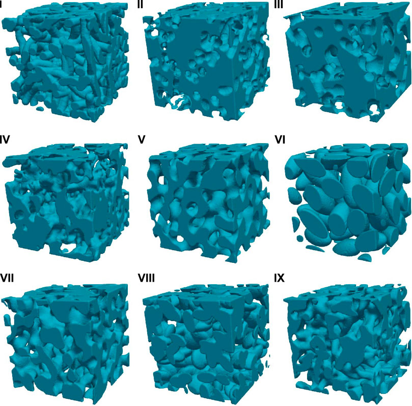
FIGURE 1. Examples of the different types of microstructures, showing an artificially generated fiber system (I), channel system (II), spatial graph (III), level set of a Gaussian random field (IV), level set of a spinodal decomposition (V), as well as systems of hard ellipsoids (VI), smoothed hard ellipsoids, (VII), soft ellipsoids (VIII), and smoothed soft ellipsoids (IX). Note that the solid phase is always depicted in blue, whereas mass transport takes place in the transparent porous phase.

FIGURE 2

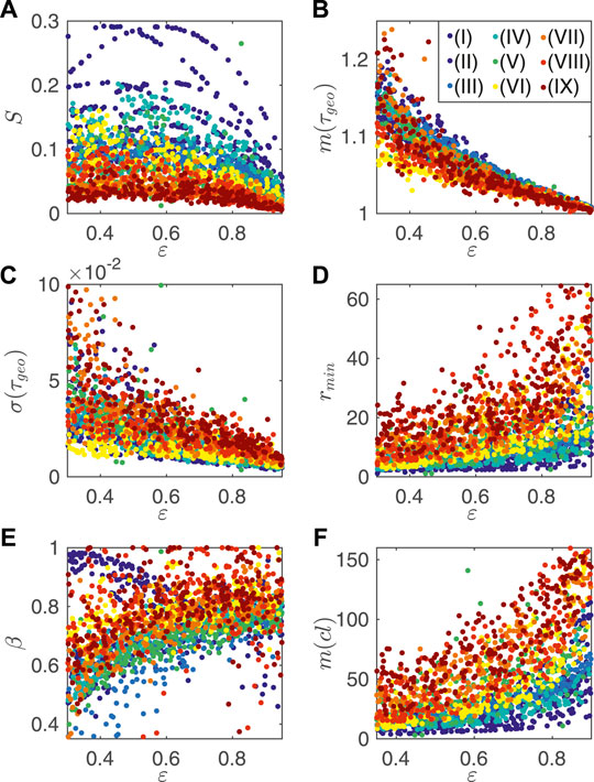
FIGURE 2. Specific surface area (in (voxelunit)⁻¹) (A), mean geodesic tortuosity (B), standard deviation of geodesic tortuosity (C), characteristic bottleneck radius r_min (in voxelunit) (D), constrictivity (E) and mean chord length (in voxelunit) (F) as a function of porosity, where 250 structures have been randomly selected for each of the nine different microstructure models, depicted by nine distinct colors. Note that the roman numbers in the legend correspond to the numbering of the nine stochastic model types mentioned at the beginning of Section 4.

4.1 Fiber Systems

The fiber systems considered in this paper are generated using essentially the method described in Townsend et al. (2021), with modifications to allow for periodic and isotropic structures. Individual fibers are first represented as a set of nodes generated by a random walk. The angle between the directions of two consecutive steps of the random walk are drawn from a spherical von Mises distribution (Mardia and Jupp, 1999). The parameters of the von Mises distribution are the mean direction μ_dir, which is computed using the angle between the previous two nodes, and the concentration θ_dir, which specifies the global bending tendency of the fibers. The random walks have a fixed length of 8 nodes. The step length is drawn from a normal distribution with mean 16 voxels and standard deviation 2 voxels. To generate the skeleton of a fiber, we plot a smooth Bézier curve (Gallier, 2000) through its node points. A curvature parameter ρ for the Bézier curves controls the local bending tendency of the fibers. This skeleton is discretized on the 192³ voxel grid and then dilated to obtain the final cylindrical fibers with radius r, subject to periodic boundary conditions. The concentration parameter θ_dir and the curvature ρ are drawn from the uniform distribution on the intervals (Torquato, 2002; Furat et al., 2021) and [0.25, 0.75], respectively. Furthermore, the fiber radius r is drawn at random from the set of integers {2, 3, 4, 5, 6, 7, 8}. Starting from a fully porous structure (without any fibers), new fibers are added until the desired porosity is reached. The method is implemented in MATLAB (2021).

4.2 Channel Systems

Systems of channels are generated using essentially the same code as for the fiber systems considered in Section 4.1, treating the fibers as porous channels instead. The parameters of the random walks, the Bezier curves, and the fiber radii are sampled in the same fashion as in Section 4.1. Starting from a fully solid structure (without any channels), new channels are added until the desired porosity is reached.

4.3 Spatial Stochastic Graphs

Spatial stochastic graph structures are generated using a model that has been introduced in Gaiselmann et al. (2014), where it has been applied to mimic the 3D microstructure of solid oxid fuel cells. The spatial graph model is based on a homogeneous Poisson point process $X={\{X_n\}}_{n\in \mathbb{N}}$ with parameter λ > 0 (Last and Penrose, 2017), where $\lambda =\mathbb{E}\#\{n\in \mathbb{N}:X_n\in {[\mathrm{0,1}]}^3\}$ is the expected number of points per unit volume, with #A denoting the cardinality of a set A. Note that by this frequently used point-process model the situation of complete spatial randomness is depicted, i.e., there is no interaction between the points X_n. For a more formal introduction to the concept of point processes, the reader is referred, e.g., to the monographs of Daley and Vere-Jones (2005) and Daley and Vere-Jones (2008). Next, the relative neighborhood graph G_X = (X, E_X) (Toussaint, 1980) is constructed, where the set X of vertices is given by the atoms X_n of the underlying homogeneous Poisson process. In order to define the edge set E_X, a so-called critical region $R(p_1,p_2)=B(p_1,‖p_1-p_2‖)\cap B(p_2,‖p_1-p_2‖)$ for $p_1,p_2\in {\mathbb{R}}^3$ is considered, where ‖p‖ denotes the Euclidean norm of $p\in {\mathbb{R}}^3$. The edge set E_X is now given by E_X = {(X_i, X_j) ∈ X × X: #(R(X_i, X_j) ∩ X) = 2}, This means that there is an edge between two points X_i and X_j if and only if there is no further point of X within the critical region R(X_i, X_j) except for X_i and X_j themselves. Finally, each edge e ∈ E_X is dilated using a sphere as structuring element (Soille, 2003). The radius of the sphere follows a Gamma distribution with expectation μ_Γ and variance ${\sigma }_{\mathrm{\Gamma }}^2$, where each edge is dilated independently from the other edges. In order to obtain an approximately uniformly distributed porosity between 0.3 and 0.95, we draw the model parameters λ, μ_Γ and ${\sigma }_{\mathrm{\Gamma }}^2$ from the uniform distribution on the intervals [10^–5, 5 ⋅ 10^–4], [1, 10] and [1, 6], respectively. Then, after generating 25,000 samples of such microstructures, it was possible to select 10,000 of them leading to the desired uniform distribution of porosities on the interval [0.3, 0.95]. The generation of 3D microstructures by the spatial stochastic graph model described above is carried out by in-house Java software using the Geostoch framework (Mayer et al., 2004).

4.4 Level Sets of Gaussian Random Fields

Level sets of Gaussian random fields are a well-known concept of stochastic geometry (Lantuéjoul, 2002; Chiu et al., 2013) which, among others, is used for modeling the 3D microstructure of anodes in lithium-ion batteries (Kremer et al., 2020) and electrodes in solid oxide cells (Moussaoui et al., 2018). In the present paper, periodic Gaussian random fields are generated using an approach based on the fast Fourier transform (FFT) (Lang and Potthoff, 2011). It utilizes the spectral density of the covariance function to generate a random field with the desired covariance structure. In particular, zero-centered white noise (independent and normal distributed) is generated in the spatial domain, transformed to the Fourier domain, and multiplied by the square root of the spectral density, where four types of spectral densities (power-law, exponential, Gaussian, and circular top-hat) are used to generate 2,500 structures of each kind (Röding et al., 2020). After linear rescaling and applying inverse FFT, a Gaussian random field with mean zero and the specified covariance function is obtained. The parameters of the different spectral densities are chosen to ensure a suitable range of length scales. Finally, binary microstructures are obtained as level sets of the random fields, i.e., the desired porosities are obtained by thresholding at appropriate quantiles of the Gaussian random field intensity distributions. The method is implemented in MATLAB (2021).

4.5 Level Sets of Spinodal Decompositions

Phase separation dynamics through the spinodal decomposition mechanism are simulated by solving a system of Navier-Stokes and Cahn-Hilliard equations (Miranville, 2019). A field of spatially resolved concentrations, denoted by $\psi \left(\mathbf{x},t\right)\in [\mathrm{0,1}]$, is evolved in time using the lattice Boltzmann method (Krüger et al., 2017). Initially, the values of ψ are uniformly distributed in the interval [0, 1], independently for all grid points on a 96³ grid. The spatiotemporal evolution of the concentration profile is determined by several factors such as surface tension, density and viscosity ratio between the two phases. These three characteristics are chosen log-uniformly distributed in their respective ranges to yield a slightly different behaviour of the interfacial geometry. Furthermore, the numbers of time steps, which control the degree of coarsening of the structures, are chosen such that a suitable range of length scales is obtained. Note that the Lifshitz-Slyozov law states that the typical length scale in the structure is proportional to the cubic root of the simulation time (Lifshitz and Slyozov, 1961). After terminating the simulations, the solutions are upscaled to 192³ voxels. Finally, in the same way as described in Section 4.4 for Gaussian random fields, the desired porosities are obtained by thresholding at appropriate quantiles of the concentration intensity distributions. The spinodal decomposition simulations are implemented using in-house software based on the lattice Boltzmann method (Gebäck and Heintz, 2014; Gebäck et al., 2015).

4.6 Hard Ellipsoids

Configurations of hard (i.e., non-overlapping) ellipsoids have been used as models for e.g., separation columns (Bertei et al., 2014) and are simulated using a hard-particle Markov Chain Monte Carlo (MCMC) algorithm (Brooks et al., 2011). Initially, the ellipsoids are placed at random locations and with random orientations. Then, the configurations are relaxed by performing random translations and rotations of all particles until no pairs of particles overlap. If the desired porosity is larger than 0.5, non-overlapping configurations can be generated easily at constant porosity as described above. Otherwise, as a preliminary procedure, the steps described above are performed for a porosity of 0.5 and then the resulting configuration is compressed in small steps, until the target porosity is reached. The magnitudes of proposed translations and rotations are adaptively selected such that the acceptance probability is held at 0.25. The number of ellipsoids is between 8 and 512, yielding a wide range of length scales. In addition, the ellipsoids are given by vectors of semi-axes (1, 1, α) where the random variable α is uniformly distributed in the interval [0.25, 1] (oblate) with probability 0.5 and, otherwise, uniformly distributed in [1, 4] (prolate). The microstructures drawn from this model are generated using in-house developed software (Röding, 2017; Röding, 2018) implemented in Julia (Bezanson et al., 2017).

4.7 Smoothed Hard Ellipsoids

Configurations of smoothed hard ellipsoids are generated in the same manner as the hard ellipsoid systems described in Section 4.6, with the only difference that the final discretized structure is smoothed with a Gaussian filter, the standard deviation of which is randomly sampled in the range of [2, 16] voxels (Gonzalez and Woods, 2008; Russ, 2007). This yields structures with a semi-continuous solid phase in contrast to the systems of hard ellipsoids described in Section 4.6, which consist of discrete particles. Note that similar structures have been used in Prill et al. (2017) as a model for porous electrodes, where spheres instead of random ellipsoids are considered.

4.8 Soft Ellipsoids

Configurations of soft (i.e., overlapping) ellipsoids are created in a similar fashion as the systems of hard ellipsoids considered in Section 4.6, but without implementing a specific overlap criterion. Instead, ellipsoids with random locations and orientations are sequentially added until the desired porosity has been obtained. The ellipsoid sizes relative to the simulation window are selected at random to yield an appropriate range of length scales. As in the case of hard ellipsoid systems considered in Section 4.6, soft ellipsoids are given by vectors of semi-axes (1, 1, α), where α is uniformly distributed in [0.25, 1] (oblate) with probability 0.5 and, otherwise, uniformly distributed in [1, 4] (prolate). The method is implemented in Bezanson et al. (2017).

4.9 Smoothed Soft Ellipsoids

Configurations of smoothed soft ellipsoids are generated in the same manner as the systems of soft ellipsoids considered in Section 4.8, with the only difference that the final discretized structure is smoothed with a Gaussian filter, the standard deviation of which is randomly sampled in the range of [2, 16] voxels (Russ, 2007; Gonzalez and Woods, 2008). This yields structures with a smoother, more continuous solid phase.

5 Microstructure-Property Relationships

For the 90,000 samples of 3D microstructures generated by the stochastic models described in Section 4, the structural descriptors explained in Section 2 as well as the effective transport properties stated in Section 3 are computed. This data is then used to establish microstructure-property relationships by means of three different approaches, namely analytical prediction formulas, (artificial) fully-connected neural networks (ANNs) and convolutional neural networks (CNNs). For this, the data is randomly shuffled and split into three subsets of training, validation, and test data, respectively. This is done in a stratified manner such that an equal number of microstructures of each type is included in each of the three datasets. The split, which is the same for each of the three types of prediction models, is 70% training data (7,000 per type of microstructure and 63,000 in total) and 15% each for the validation and test data (1,500 per type of microstructure and 13,500 in total).

Several error measures are considered to assess predictive performance. For fitting the prediction models, the mean squared error (MSE) loss is used, where

$\mathrm{M}\mathrm{S}\mathrm{E}=\frac{1}{k}\sum _{j=1}^k{({\widehat{y}}_j-y_j)}^2.(6)$

Here y₁, … , y_k is the ground truth data of a given output variable and ${\widehat{y}}_1,\dots ,{\widehat{y}}_k$ are the corresponding estimates predicted by the model. Depending on context, the MSE loss is used either on the output variables themselves or on transformed outputs. Further details can be found below in Sections 5.1–5.3 for the three types of microstructure-property relationships considered in this paper. Note that the MSE loss is an appropriate loss function for optimization because it is differentiable. In contrast, for final assessment, the mean absolute percentage error (MAPE) loss is used, where

$\mathrm{M}\mathrm{A}\mathrm{P}\mathrm{E}=\frac{100}{k}\sum _{j=1}^k\left|\frac{{\widehat{y}}_j-y_j}{y_j}\right|.(7)$

However, because the MAPE loss is not everywhere differentiable, it is less well-behaved as an optimization target, but on the other hand it is more interpretable.

In addition, we consider the coefficient of determination R² ∈ [0, 1], which is given by

$R^2=1-\frac{\sum _{j=1}^k{(y_j-{\widehat{y}}_j)}^2}{\sum _{j=1}^k{(y_j-\bar{y})}^2},(8)$

where $\bar{y}$ denotes the empirical mean of the ground truth data y₁, … , y_k. Since the values for permeability cover several orders of magnitude, the value of R² would be dominated by those terms that involve large values. For this reason, we also consider the coefficient of determination on the log scale, denoted by $R_{\log }^2\in [\mathrm{0,1}]$. In particular, it holds

$R_{\mathit{log}}^2=1-\frac{\sum _{j=1}^k{(\log (y_j)-\log ({\widehat{y}}_j))}^2}{\sum _{j=1}^k{(\log (y_j)-{\bar{y}}_{\log })}^2},(9)$

where ${\bar{y}}_{\log }$ is defined as the empirical mean of the sample log(y₁), …, log(y_k).

Before the derivation of microstructure-property relationships is discussed, we first quantify the “amount of information” that is contained in the different structural descriptors with regard to permeability, effective tortuosity and the M-factor. For this purpose, we make use of the measure of general functional dependence, which has been introduced in (Xu et al., 2017). In contrast to several widely used quantities such as Pearson’s ρ, Kendall’s τ or Spearman’s ρ, this characteristic, denoted by 0 ≤ δ(x, y) ≤ 1, relies neither on a linear nor on a monotone relationship between the quantities x and y. Thus, it can be used to quantify the importance of a single (scalar) structural descriptor x on an effective property y, where higher values correspond to a higher “amount of information”. The upper limit of 1 is reached if and only if x is a function of y or vice versa since in general it holds δ(x, y) = δ(y, x). The corresponding results are shown in Table 1. Note that the values for the effective tortuosity are always larger than for the M-factor, which is probably caused by the fact that τ_eff already contains the porosity ɛ. However, it is worth mentioning that a low value of the functional dependence measure does not automatically imply that this quantity should not be considered for predicting a certain effective property. This is due to the fact that δ(x, y) only contains some information on the predictive power of x with regard to y, but not regarding the usefulness of x in combination with other structural descriptors. This also explains the fact that the normalized quantity M turned out to be predicted with higher accuracy than τ_eff, and therefore we stick to M for the rest of this work. It is also interesting to point out that m(L) and σ(L) seem to be closely related to permeability and effective tortuosity, considering that the chord length distribution is rarely used in the literature for establishing microstructure-property relationships.

TABLE 1

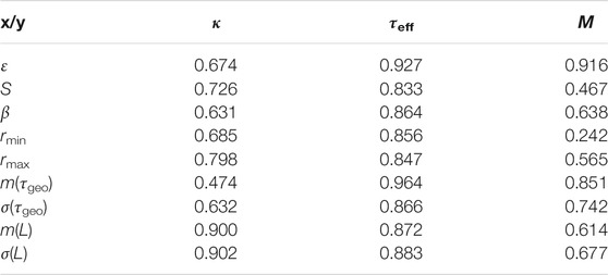
TABLE 1. Functional dependence measure δ(x, y) between a scalar structural descriptor x and an effective property y.

5.1 Analytical Prediction Formulas

In this section, microstructure-property relationships are derived by analytical prediction formulas, whose parameters are fitted by least-squares regression (Sen and Srivastava, 2012). More precisely, we use the trust-region-reflective algorithm (Coleman and Li, 1994; Coleman and Li, 1996) for unconstrained least-squares problems and the interior point algorithm (Byrd et al., 2000; Waltz et al., 2006) for constrained ones. Since there are no hyperparameters in case of analytical prediction formulas, we merge the training set with the validation set for computing the fitting parameters and use the test set for assessing performance. Altogether, we state nine analytical prediction formulas and their fitting parameters. Afterwards, a comparison of these formulas is carried out, including an interpretation of the results.

To begin with, we consider several relationships between geometric microstructure descriptors given in Section 2 and the M-factor stated in Section 3. Recall that according to Equation 21.14 in the book of S. Torquato (Torquato, 2002), it holds that M ∈ [0, 1], which is also ensured for the predictions $\widehat{M}$ of M presented below. At first, we consider a type of a parametric formula, which has been originally proposed in Stenzel et al., 2016) and later reconsidered in Eq. 4 of Neumann. et al. (2020). More precisely, the M-factor is predicted by

$\widehat{M}={\epsilon }^{c_1}{\beta }^{c_2}m{({\tau }_{\text{geo}})}^{c_3}.(10)$

To ensure that $\widehat{M}\in [\mathrm{0,1}]$, we use the constraints c₁ ≥ 1 and c₂ ≥ 0, which leads to the following results: c₁ = 1, c₂ = 0 and c₃ = − 8.45. More precisely, the best fit in a least-squares sense does not contain the constrictivity β, whereas the exponent of the porosity equals the lower limit of one. Note that Formula (Eq. 10) for predicting the M-factor has been modified in Neumann. et al. (2020) to ensure that $\widehat{M}\in [\mathrm{0,1}]$ holds also for the dilute limit by using the constrictivity β within the exponent of porosity. More precisely, in Neumann. et al. (2020) the following parametric prediction formula is proposed:

$\widehat{M}={\epsilon }^{c_1+c_2\beta }m{({\tau }_{\text{geo}})}^{c_3},(11)$

where the additional constraint c₁ + c₂ ≥ 0 is used to ensure that $\widehat{M}\in [\mathrm{0,1}]$. This leads to c₁ = 1.25, c₂ = − 1.25 and c₃ = − 7.82. Finally, we consider a formula for predicting the M-factor by porosity as well as the mean and standard deviation of geodesic tortuosity of the pore space, see Barman et al. (2019):

$\widehat{M}=c_{1}m{({\tau }_{\text{geo}})}^{c_2}\sigma {({\tau }_{\text{geo}})}^{c_3}{\epsilon }^{c_4},(12)$

where least-squares fitting gives that c₁ = 1.18, c₂ = − 9.17, c₃ = 0.03 and c₄ = 1.02.

Having discussed parametric formulas for predicting the M-factor, we now predict the permeability κ using geometric microstructure descriptors given in Section 2. Since the values of κ can cover several orders of magnitude, the fitting of parameters is carried out on the log scale. First, we consider the prediction formula

$\widehat{\kappa }=c_1{\epsilon }^{c_2}{\beta }^{c_3}{S}^{-2}m{({\tau }_{\text{geo}})}^{c_4},(13)$

which has been introduced in Neumann. et al. (2020). By least-squares regression, we obtain that c₁ = 0.16, c₂ = 2.05, c₃ = 0.64 and c₄ = − 7.31. Moreover, we consider still another type of a parametric prediction formula for κ, proposed in Neumann. et al. (2020). Namely,

$\widehat{\kappa }=c_1{(c_2{r}_{\text{min}}+c_3{r}_{\text{max}})}^2{\epsilon }^{c_4}m{({\tau }_{\text{geo}})}^{c_5},(14)$

where least-squares fitting gives that c₁ = 0.24, c₂ = 0.92, c₃ = 0.08, c₄ = 1.6 and c₅ = − 6.82. Note that for fitting the parameters in Eq. 14 we use the additional constraint c₂, c₃ ∈ [0, 1] with c₂ + c₃ = 1. Thus, we use a convex combination of r_min and r_max, which is subsequently squared to ensure the right unit of permeability. Last not least, a further parametric prediction formula for κ, which has been discussed in the literature, is given by

$\widehat{\kappa }=c_1{\epsilon }^{c_2}{S}^{-2}m{({\tau }_{\text{geo}})}^{c_3},(15)$

see Röding et al. (2020), where least-squares regression leads to c₁ = 0.14, c₂ = 2.07 and c₃ = − 8.57.

In addition to the results mentioned above, we consider the following prediction formula for κ:

$\widehat{\kappa }=c_1{\epsilon }^{c_2+c_3\beta }{S}^{-2}m{({\tau }_{\text{geo}})}^{c_4},(16)$

which uses the constrictivity β within the exponent of the porosity ɛ, similar to Eq. 11, where the fitting parameters are given by c₁ = 0.14, c₂ = 3.07, c₃ = − 1.38 and c₄ = − 7.37. Furthermore, we predict κ by the porosity ɛ, the mean geodesic tortuosity m(τ_geo) and the median r_min via

$\widehat{\kappa }=c_1{\epsilon }^{c_2}m{({\tau }_{geo})}^{c_3}{r}_{min}^2,(17)$

where least-squares fitting on the log scale gives that c₁ = 0.25, c₂ = 1.6 and c₃ = − 6.6. Finally, we consider a prediction formula for κ which involves the mean chord length m(L) of the pore space:

$\widehat{\kappa }=c_{1}m{(L)}^{c_2}{\epsilon }^{c_3+c_4\beta }{r}_{\text{min}}^{c_5}m{({\tau }_{\text{geo}})}^{c_6},(18)$

where we use the constraint c₂ + c₅ = 2 in order to obtain the right unit (voxels²), and the fitting parameters are given by c₁ = 0.1, c₂ = 0.63, c₃ = 1.38, c₄ = − 0.2, c₅ = 1.37 and c₆ = − 6.74.

Regarding the prediction of effective diffusivity, the data visualized in the top row Figure 3 lead to the following results. It is interesting to observe that the problem of Eq. 10 described in Neumann. et al. (2020), namely not fulfilling that $\widehat{M}\approx 1$ in the dilute limit (ɛ → 1), does not occur, see Figure 3A, since fitting the coefficients leads to c₂ = 0, i.e., the constrictivity β is not used for predicting effective diffusivity. Furthermore, note that the performance of Eq. 10 is similar to the performance of Eqs. 11, 12 even though the latter one does not involve constrictivity, see Figures 3A–C.

FIGURE 3

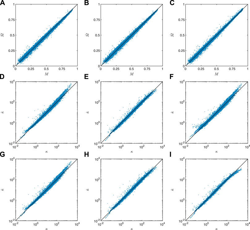
FIGURE 3. Prediction of effective transport properties using analytical formulas. Top row (from left to right): Prediction of M-factor via Eqs. 10–12. Middle row (from left to right): Prediction of permeability via Eqs. 13–15. Bottom row (from left to right): Prediction of permeability via Eqs. 16–18. Note that the scatter plots show results based on the test data.

In contrast to the prediction of effective diffusivity, the performance of the analytical prediction formulas for permeability significantly varies case by case, see Figures 3D–I. In particular, Eq. 15 leads to the lowest predictive power in terms of MAPE, where the low value of the coefficient of determination R² is attributed to an overestimation of permeability in the regime of large permeability values, see Table 2. This also holds with regard to Eqs. 13, 16, which both lead to a similar MAPE of approximately 18%. On the other hand, a remarkable improvement can be observed by disregarding constrictivity and including instead r_min, as in Eq. 17, or a convex combination of r_min and r_max, as in Eq. 14, where both prediction formulas lead to a MAPE of approximately 15%. However, it is worth mentioning that Eq. 17 only uses three adjustable parameters and three geometric descriptors of the underlying 3D microstructure. In addition, the small value c₃ = 0.08 of the parameter corresponding to r_max in Eq. 14 highlights the importance of the direction-dependent characteristic r_min, which in contrast to r_max also contains information about bottleneck effects. The best performance with regard to MAPE is obtained when additionally using the mean chord length as in Eq. 18, where one has to note that this prediction formula also contains the highest number of parameters as well as microstructure descriptors. However, it is interesting to note that such a simple quantity as the mean chord length turns out to be beneficial in terms of further improving the predictive power see Table 2.

TABLE 2

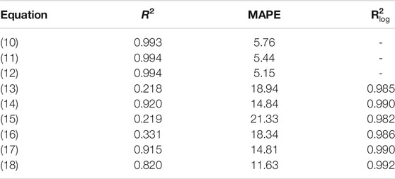
TABLE 2. Error measures computed on the test set, corresponding to the analytical prediction formulas Eqs. 10–18 for M-factor and permeability, respectively. Note that in case of predicting permeability, the quantity $R_{\log }^2$ denotes the coefficient of determination on the log scale.

5.2 Artificial Neural Networks

In addition to the analytical prediction formulas Eqs. 10–18 presented above, we investigate artificial neural networks (ANNs) for the prediction of mass transport properties. Note that a conventional, fully-connected ANN is a composition of linear and nonlinear operations. The building blocks are fully-connected (also called dense) layers, each of which consists of a certain number of nodes. The input to each node is a weighted sum of the outputs from the nodes in the previous layer, to which a nonlinear so-called activation function $f:\mathbb{R}\to \mathbb{R}$ is applied. As a whole, the network describes a nonlinear mapping from some input to some output that can be arbitrarily complex. During training of an ANN, the parameters (weights of the sums) are optimized with respect to a loss function that penalizes deviations from the target output (Schmidhuber, 2015).

The first layer is, in a sense, the input layer, the dimension of which depends on the set of microstructural descriptors used. The first layer is followed by a certain number of fully-connected layers, so-called hidden layers, which are described below in more detail. The final layer is the output layer, which in our case of a scalar output consists of a single node only. For the hidden layers, the exponential linear unit (Elu) activation function is used (Clevert et al., 2016), which is given by

$f(x)=\left\{\begin{array}{cc}x,\hfill & \text{if\hspace{0.17em}}x>0\text{,}\hfill \\ \gamma \left(e^x-1\right),\hfill & \text{if\hspace{0.17em}}x\le 0\text{,}\hfill \end{array}\right.(19)$

where we put γ = 1.

We investigate 12 different sets of geometric microstructure descriptors, re-using all sets of descriptors considered in the analytical prediction formulas Eqs. 10–18 and also adding new ones involving more complex descriptors like distributions/quantiles of e.g., geodesic tortuosity, chord length distributions, spherical contact distribution and the two-point correlation function. The descriptor sets are summarized in Table 3. The inputs, i.e. the microstructure descriptors, are linearly rescaled such that in each case, the input data provided by the training set has zero mean and unit variance, which often improves convergence during training (LeCun et al., 2012). Furthermore, the outputs are transformed in the following fashion. The values of M ∈ (0, 1) and κ ∈ (0, ∞) cover some orders of magnitude. To simplify training, the logit-transformed M-factor y = log(M/(1 − M)) and the log-transformed permeability y = log(κ) are used as the target outputs. This yields the benefit that the inverse-transformed predictions belong to (0, 1) and (0, ∞), respectively.

TABLE 3

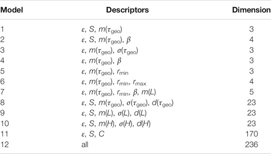
TABLE 3. Descriptor sets used as input for the ANNs, together with the dimensions of the corresponding input vectors. Note that Models 8, 9 and 10 involve four scalar quanities and one distributional characteristic described by 19 quantiles, whereas the two-point correlation function in Model 1 is evaluated for 168 different radii.

The networks are implemented in Tensorflow 2.4.1 (Abadi et al., 2015) and optimized with respect to MSE loss (on the logit and log scales). Glorot/Xavier uniform initialization is used for all weights (Glorot et al., 2010), as well as stochastic gradient descent (SGD) with momentum (Qian, 1999; Bottou, 2010) for optimization. A random search hyperparameter optimization (Bergstra and Bengio, 2012) is performed to quantify the importance of the number of hidden layers, the number of nodes per layer, the batch size (in each update in the SGD), the momentum and the learning rate of the SGD. It turns out that 4 hidden layers, each with 64 nodes, is a reasonable choice, where the number of weights varies from 12,801 to 27,713 depending on the dimension of the descriptor input. The network architecture is illustrated in Figure 4. Furthermore, a batch size of 128 and a momentum of 0.9 is chosen, but those particular values turned out to be not critical with regard to the performance. Also, we consider different kinds of regularization such as weight decay, i.e., l₂ regularization (Krogh and Hertz, 1992) and dropout regularization (Srivastava et al., 2014), where both did not lead to any improvement. It is also worth mentioning that batch normalization (Ioffe and Szegedy, 2015), another common regularization method, is not investigated here because combining it with the Elu activation function (Clevert et al., 2016) has been found not useful. Finally, it turned out that the learning rate (LR) has considerable impact on the results. Therefore, we design an LR scheme with a step-wise increasing and then step-wise decreasing learning rate. More precisely, let LR ∈ {10^–4.5, 10^–4, 10^–3.5, 10^–3, 10^–2.5} for 1,000 epochs (iterations over the whole training set) each, and then, we choose LR ∈ {10^–2, 10^–2.5, 10^–3, 10^–3.5, 10^–4} for 4,000 epochs each. In total, the training procedure comprises 25,000 epochs. For each set of inputs, i.e., microstructural descriptors, 100 networks are trained using different random seeds. Note that the random seed controls the weight initializations in the network as well as the shuffling of data in the SGD. The model yielding the minimal validation loss (over all epochs and all runs) for each set of microstructural descriptors is selected. On a single NVIDIA T4 GPU, the average execution time for each run is 3.7 h.

FIGURE 4

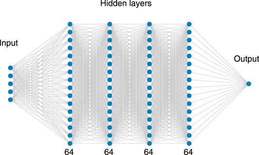
FIGURE 4. Illustration of the ANN architecture with 4 hidden layers, each with 64 nodes, where only a smaller number of nodes is shown in this figure for clarity. Furthermore, the input in this figure is 5-dimensional, but in the present paper the input dimension varies from 3 to 236, see Table 3.

Scatter plots visualizing the prediction results for M-factor and permeability are shown in Figures 5, 6, respectively. Furthermore, error measures for the prediction of M-factor and permeability are shown in Tables 4 and 5, respectively. It turns out that the predictions obtained by ANNs are consistently better than those obtained by the analytical prediction formulas considered in Section 5.1, when the same descriptors are used as input. In addition, adding more complex descriptors like quantiles (of tortuosity, etc.) improves the results even further. Unsurprisingly, the best results are obtained using all the computed descriptors.

FIGURE 5

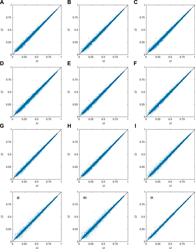
FIGURE 5. Prediction of M-factor using ANNs. Top row (from left to right): Prediction of M via Models 1–3. Second row (from left to right): Prediction of M via Models 4–6. Third row (from left to right): Prediction of M via Models 7–9. Bottom row (from left to right): Prediction of M via Models 10–12. Note that the scatter plots show results based on the test data.

FIGURE 6

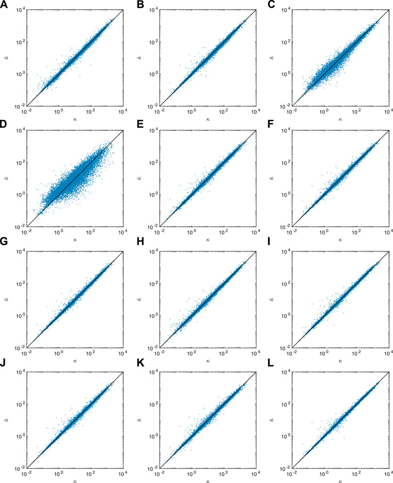
FIGURE 6. Prediction of permeability using ANNs. Top row (from left to right): Prediction of κ via Models 1–3. Second row (from left to right): Prediction of κ via Models 4–6. Third row (from left to right): Prediction of κ via Models 7–9. Bottom row (from left to right): Prediction of κ via Models 10–12. Note that the scatter plots show results based on the test data.

TABLE 4

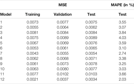
TABLE 4. Error measures for the prediction of M via ANNs where MSE is given for the training, validation and test sets, and MAPE for the test set. Note that MSE is evaluated on the logit scale and MAPE on the linear scale.

TABLE 5

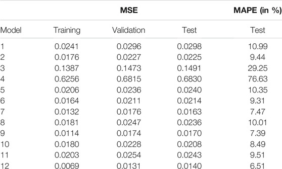
TABLE 5. Error measures for the prediction of κ via ANNs, where MSE is given for the training, validation and test sets, and MAPE for the test set. Note that MSE is evaluated on the logit scale and MAPE on the linear scale.

Note that some of the ANN models (Models 1–7 in Table 3) involve exactly the same sets of descriptors as input which are used in the analytical models for the prediction of M and/or κ. Not surprisingly, the ANNs outperform the corresponding analytical prediction formulas (with the same descriptor sets) in all cases in terms of MAPE evaluated on the test set. Furthermore, in the case of geodesic tortuosity τ_geo, there are clear improvements when adding more detailed information on the distribution of τ_geo, i.e., starting with ϵ, m(τ_geo), σ(τ_geo) and then adding 19 quantiles of d(τ_geo), the MAPE is reduced from 3.84 to 3.38% for the M-factor, and from 29.25 to 10.01% for permeability. Also, descriptor sets involving detailed information on the distributions of chord lengths and spherical contact distances perform well. With regard to the prediction of the M-factor, these high-dimensional descriptors perform better than the ANN model (no. 10 in Table 3) involving the two-point correlation function. However, for the prediction of permeability, the ANN model involving the two-point correlation function performs better than the model (no. 8) involving the distribution of tortuosity.

Note that the Models 3 and 4 which do not use neither r_min nor the specific surface area S, perform substantially worse than all other models with regard to permeability. Not surprisingly, including all descriptors (Model 12) yields the best performance for predicting both M and κ. However, comparing models with low-dimensional (Models 1–7) and high-dimensional (Models 8–12) descriptor sets, the best low-dimensional descriptor (Model 7) gives very good performance. In particular, going from 5 to 236 input dimensions reduces the MAPE from 2.74 to 2.03% for M and from 7.47 to 6.51% with regard to κ. Considering that this reduction in error requires a massive reduction in interpretability of the model, it is not obvious how to make this trade-off between model complexity and performance.

5.3 Convolutional Neural Networks

In a CNN, as opposed to a conventional ANN, the main building blocks are convolutional layers. A typical CNN architecture comprises convolutional layers, pooling layers, and fully-connected layers. In the convolutional layers, the input is convolved with several convolution kernels, whose entries are trainable parameters. The convolutions themselves are linear operations, but a nonlinear activation function $f:\mathbb{R}\to \mathbb{R}$ is applied to the result to produce the outputs, called feature maps. In the pooling layers, the feature maps are downsampled by computing, e.g., the mean or maximum on small (typically non-overlapping) patches of the feature maps from the preceding layer, reducing the resolution such that the next convolutional layer can extract information from another spatial scale. After the convolutional and pooling layers, fully-connected layers are typically used to obtain a scalar output. The first part of the CNN can be thought of as a feature extractor that produces geometrical features which are qualitatively similar to the ones used for the analytical prediction formulas and ANNs considered in the previous sections of this paper, whereas the second part corresponds directly to the ANNs themselves.

The size of the microstructures themselves is too large to be practically feasible from a computational point of view. Therefore, we downsample to half the size in all directions by averaging. The result is a 96³ array for each structure with values in {0, … , 8} stored as 8-bit unsigned integers. Apart from a linear scaling factor, this preprocessing step is equivalent to having an average pooling filter with a 2 × 2 × 2 window as the first layer in the CNN. Preprocessing the structures in this manner allows for a larger batch size without running out of GPU memory. During training, the input arrays are batch-wise converted to 32-bit floating point precision and rescaled to [ − 1/2, 1/2] prior to the gradient update. The outputs are transformed in the same way as for the ANNs. The first part of the CNN consists of three convolutional blocks, each with two convolutional layers with Elu activations and one average pooling layer. The convolutional layers use 3 × 3 × 3 kernels, and the number of filters, i.e. kernels, used is 16, 32, and 64 in the respective blocks. The average pooling layers use 2 × 2 × 2 windows. The second part of the CNN consists of 4 fully-connected layers with Elu activations, each with 64 nodes, i.e. the same as for the ANNs considered in the previous section. The total number of weights is 2,324,689. The network architecture is illustrated in Figure 7.

FIGURE 7

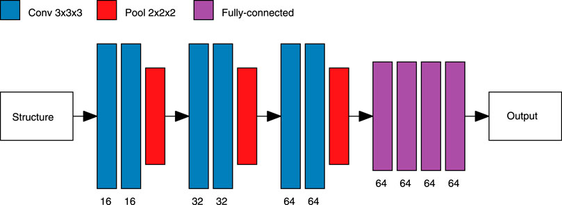
FIGURE 7. Illustration of the CNN architecture. The inputs, arrays of size 96³, are fed into the convolutional part of the network, consisting of three convolutional blocks, each in turn consisting of two convolutional layers (the numbers of filters are indicated in the figure) followed by an average pooling layer. The feature maps produced as output from the convolutional part are passed to 4 fully-connected layers with 64 nodes each.

The weight initialization procedure, optimizer, and momentum are the same as for ANNs. However, the batch size is 16 and the learning rate (LR) schedule is also different: Let LR ∈ {10^–4, 10^–3.75, 10^–3.5, 10^–3.25} for 25 epochs each, then LR = 10^–3 for 100 epochs, and finally LR ∈ {10^–3.25, 10^–3.5, 10^–3.75, 10^–4} for 50 epochs each, in total comprising 400 epochs. In contrast to ANNs, we now introduce a data augmentation scheme for the training data, involving random flips, rotations, and circular shifts of the structure array in both dimensions orthogonal to the mass transport direction. The mass transport is invariant with respect to these transformations such that a data augmentation scheme like this will act as a regularizer that increases the generalization performance of the network (Hernández-García et al., 2018). On a single NVIDIA V100 GPU, the average execution time is 140 h. The model yielding the minimal validation loss over all epochs is selected. Because of the large computational workload for CNNs, we do only one run for M-factor and one for permeability.

In addition to this ordinary CNN, we train the same architecture with a different kind of input data. Instead of using the structure arrays, we compute the Euclidean distance transform in the pore space which effectively comprises a spatial map of local pore sizes (Russ, 2007). To the best of our knowledge, this approach of using the distance transform as a representation of the pore space has not been used before as inputs to a CNN, where these inputs are again rescaled to 96³ arrays. The only differences compared to the ordinary CNN are that the input data has to be stored in 32-bit floating point precision (leading to high demands in storage space, ∼ 320 GB for training, validation, and test) and that the data are batch-wise rescaled by a factor 1/24 (the 95%-quantile of the distance transform values is approximately 24).

Scatter plots visualizing the prediction results for M-factor and permeability are shown in Figure 8. Furthermore, error measures are shown in Table 6 for both M and κ and for both the ordinary CNN (briefly denoted by CNN) and the distance-transform CNN (denoted by DT-CNN). As can be seen, all CNNs perform better than their best ANN counterparts, the best models attaining 1.65% (M-factor) and 3.78% (permeability) MAPE, although this is at the expense of even less interpretability than for the highest-dimensional descriptor used for the ANNs. Also, the differences between the ordinary CNN and the DT-CNN are not substantial and neither one of them is consistently better. This is possibly because the ordinary CNN learns similar information as that already supplied to the DT-CNN. Hence, we conclude that given the increased computational workload of the distance transform, there are at least no substantial benefits of using the DT-CNN over the ordinary CNN.

FIGURE 8

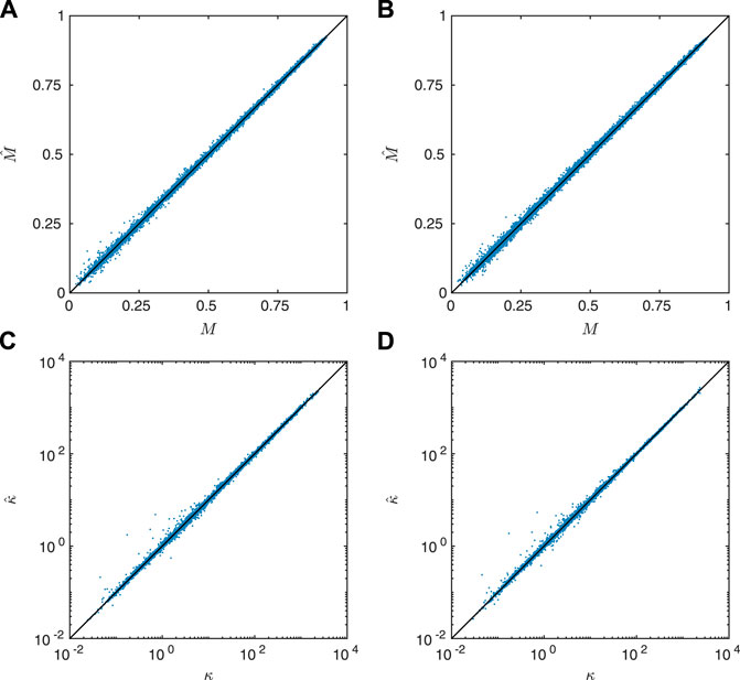
FIGURE 8. Prediction results using different CNNs, showing (A) prediction of M using an ordinary CNN, (B) prediction of M using a DT-CNN, (C) prediction of κ using an ordinary CNN, and (D) prediction of κ using a DT-CNN. Note that the scatter plots show results based on the test data.

TABLE 6

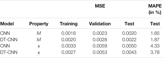
TABLE 6. Error measures for the prediction of M and κ via ordinary CNN and DT-CNN where MSE is given for the training, validation and test sets, and MAPE for the test set. Note that MSE is evaluated on the logit scale for M and log scale for κ, and MAPE on the linear scale.

6 Conclusion

We investigate microstructure-property relationships for artificially generated porous materials, developing prediction models for diffusivity and permeability based on the geometry of the pore space. The basis for this is a comprehensive dataset of 90,000 structures with size of 192³ voxels, which are generated by 9 different stochastic 3D microstructure models. To the best of our knowledge, this is the largest and most diverse dataset for studying diffusivity and permeability published so far in the literature. Microstructural descriptors like porosity, specific surface area, tortuosity and its distribution, constrictivity, spherical contact distributions, chord length distribution and two-point correlation functions are used in various combinations as input to both analytical prediction formulas and artificial neural networks (ANNs). Furthermore, the structure itself as well as a distance transform in the pore space, capturing the shortest distance to the solid phase, is used as input to convolutional neural networks (CNNs). In terms of mean absolute percentage error (MAPE), the best analytical models attain 5.15% (diffusivity) and 11.63% (permeability) error. The ANNs outperform the analytical prediction formulas with the same inputs, which indicates that the microstructure-property relationships are more complex and nonlinear than can be expressed through simple analytical models. In addition, ANNs can naturally incorporate high-dimensional descriptors like distributions (which haven been characterized by quantiles), and correlation functions. The best ANN models attain a MAPE of 2.03% (diffusivity) and 6.51% (permeability). However, one downside of ANNs is that their results are not as interpretable as those based on analytical prediction formulas. Furthermore, the CNNs outperform the best-performing ANNs, where the best CNN models attain 1.65% (diffusivity) and 3.78% (permeability) MAPE. This comes at the price of a significant increase in training time and use of computational resources, and yet another decrease in interpretability of the results. The fact that the prediction quality of best-performing ANNs comes at least reasonably close to that of CNNs indicates that the microstructural descriptors considered in this paper strongly influence mass transport and are thus suitable for predicting diffusivity and permeability. To our knowledge, analytical prediction formulas, ANNs, and CNNs have not been compared quantitatively on the same dataset before, and in particular not on such a large and diverse dataset. To facilitate further development of microstructure-property relationships, we make the artificially generated microstructures, their descriptors, and the code used to study the relationships between them available open access (Prifling et al., 2021c).

Data Availability Statement

The microstructures, descriptors, and the code used to study microstructure-property relationships are available open access via the following Zenodo repository: https://zenodo.org/record/4047774, see Prifling et al. (2021c).

Author Contributions

BP, MR and MN generated the data and performed the analysis of microstructure-property relationships. PT developed the microstructure model for fiber and channel systems. All authors discussed the results and contributed to writing the paper. VS designed and supervised the research.

Funding

The financial support of the Swedish Research Council for Sustainable Development (grant number 2019-01295) and the Swedish Research Council (grant number 2016–03809) is acknowledged. Furthermore, the presented work was financially supported by the Bundesministerium für Bildung und Forschung (BMBF) within the project HiStructures under the grant number 03XP0243D as well as by the Deutsche Forschungsgemeinschaft (DFG) under the grant number SCHM997/39-1. The computations were in part performed on resources at Chalmers Centre for Computational Science and Engineering (C3SE) provided by the Swedish National Infrastructure for Computing (SNIC). A GPU used for part of this research was donated by the NVIDIA Corporation.

Conflict of Interest

The authors declare that the research was conducted in the absence of any commercial or financial relationships that could be construed as a potential conflict of interest.

Publisher’s Note

All claims expressed in this article are solely those of the authors and do not necessarily represent those of their affiliated organizations, or those of the publisher, the editors and the reviewers. Any product that may be evaluated in this article, or claim that may be made by its manufacturer, is not guaranteed or endorsed by the publisher.

Acknowledgments

Victor Wåhlstrand Skärström is acknowledged for assistance with implementing the convolutional neural networks.

References

Abadi, M., Agarwal, A., Barham, P., Brevdo, E., Chen, Z., Citro, C., et al. (2015). TensorFlow: Large-Scale Machine Learning on Heterogeneous Systems. Available at: tensorlow.org (Accessed September 29, 2021).

Google Scholar

Abdallah, B., Willot, F., and Jeulin, D. (2016). Morphological Modelling of Three-phase Microstructures of Anode Layers Using SEM Images. J. Microsc. 263, 51–63. doi:10.1111/jmi.12374

CrossRef Full Text | Google Scholar

Allen, J., Weddle, P. J., Verma, A., Mallarapu, A., Usseglio-Viretta, F., Finegan, D. P., et al. (2021). Quantifying the Influence of Charge Rate and Cathode-Particle Architectures on Degradation of Li-Ion Cells through 3D Continuum-Level Damage Models. J. Power Sourc. 512, 230415. doi:10.1016/j.jpowsour.2021.230415

CrossRef Full Text | Google Scholar

Araya-Polo, M., Alpak, F. O., Hunter, S., Hofmann, R., and Saxena, N. (2019). Deep Learning-Driven Permeability Estimation from 2D Images. Comput. Geosci. 24, 571–580. doi:10.1007/s10596-019-09886-9

CrossRef Full Text | Google Scholar

Barman, S., Rootzén, H., and Bolin, D. (2019). Prediction of Diffusive Transport through Polymer Films from Characteristics of the Pore Geometry. AIChE J. 65, 446–457. doi:10.1002/aic.16391

CrossRef Full Text | Google Scholar

Bear, J. (2018). Modeling Phenomena of Flow and Transport in Porous Media. Theory and Applications of Transport in Porous Media. Cham: Springer.

Google Scholar

Bergstra, J., and Bengio, Y. (2012). Random Search for Hyper-Parameter Optimization. J. Mach. Learn. Res. 13, 281–305.

Google Scholar

Berryman, J. G. (1985). Bounds on Fluid Permeability for Viscous Flow through Porous media. J. Chem. Phys. 82, 1459–1467. doi:10.1063/1.448420

CrossRef Full Text | Google Scholar

Bertei, A., Chueh, C.-C., Pharoah, J. G., and Nicolella, C. (2014). Modified Collective Rearrangement Sphere-Assembly Algorithm for Random Packings of Nonspherical Particles: Towards Engineering Applications. Powder Tech. 253, 311–324. doi:10.1016/j.powtec.2013.11.034

CrossRef Full Text | Google Scholar

Bezanson, J., Edelman, A., Karpinski, S., and Shah, V. B. (2017). Julia: A Fresh Approach to Numerical Computing. SIAM Rev. 59, 65–98. doi:10.1137/141000671

CrossRef Full Text | Google Scholar

Birkholz, O., Neumann, M., Schmidt, V., and Kamlah, M. (2021). Statistical Investigation of Structural and Transport Properties of Densely-Packed Assemblies of Overlapping Spheres Using the Resistor Network Method. Powder Tech. 378, 659–666. doi:10.1016/j.powtec.2020.09.056

CrossRef Full Text | Google Scholar

Bottou, L. (2010). “Large-scale Machine Learning with Stochastic Gradient Descent,” in Proceedings of COMPSTAT’2010, Paris, France, August 22–27, 2021 (Paris: Springer), 177–186. doi:10.1007/978-3-7908-2604-3_16

CrossRef Full Text | Google Scholar

Brooks, S., Gelman, A., Jones, G., and Meng, X. (2011). Handbook of Markov Chain Monte Carlo. Chapman & Hall/CRC Handbooks of Modern Statistical Methods. Boca Raton: CRC Press.

Google Scholar

Byrd, R. H., Gilbert, J. C., and Nocedal, J. (2000). A Trust Region Method Based on Interior Point Techniques for Nonlinear Programming. Math. Program. 89, 149–185. doi:10.1007/pl00011391

CrossRef Full Text | Google Scholar

Carman, P. (1937). Fluid Flow through Granular Beds. Trans. Inst. Chem. Eng. 15, 150–166.

Google Scholar

Chiu, S. N., Stoyan, D., Kendall, W. S., and Mecke, J. (2013). Stochastic Geometry and its Applications. 3rd ed. Chichester: J. Wiley & Sons.

Google Scholar

Clennell, M. B. (1997). Tortuosity: A Guide through the Maze. Geol. Soc. Lond. Spec. Publications 122, 299–344. doi:10.1144/gsl.sp.1997.122.01.18

CrossRef Full Text | Google Scholar

Clevert, D.-A., Unterthiner, T., and Hochreiter, S. (2016). “Fast and Accurate Deep Network Learning by Exponential Linear Units (Elus),” in 4th International Conference on Learning Representations, ICLR 2016, San Juan, Puerto Rico, May 2-4, 2016. Editors Y. Bengio, and Y. LeCun. Conference Track Proceedings.

Google Scholar

Coleman, T. F., and Li, Y. (1996). An Interior Trust Region Approach for Nonlinear Minimization Subject to Bounds. SIAM J. Optim. 6, 418–445. doi:10.1137/0806023

CrossRef Full Text | Google Scholar

Coleman, T. F., and Li, Y. (1994). On the Convergence of Interior-Reflective Newton Methods for Nonlinear Minimization Subject to Bounds. Math. Programming 67, 189–224. doi:10.1007/bf01582221

CrossRef Full Text | Google Scholar

Cooper, S. J., Bertei, A., Shearing, P. R., Kilner, J. A., and Brandon, N. P. (2016). TauFactor: An Open-Source Application for Calculating Tortuosity Factors from Tomographic Data. SoftwareX 5, 203–210. doi:10.1016/j.softx.2016.09.002

CrossRef Full Text | Google Scholar

Cooper, S. J., Kishimoto, M., Tariq, F., Bradley, R. S., Marquis, A. J., Brandon, N. P., et al. (2013). Microstructural Analysis of an LSCF Cathode Using In Situ Tomography and Simulation. ECS Trans. 57, 2671–2678. doi:10.1149/05701.2671ecst

CrossRef Full Text | Google Scholar

Cybenko, G. (1989). Approximation by Superpositions of a Sigmoidal Function. Math. Control. Signal. Syst. 2, 303–314. doi:10.1007/bf02551274

CrossRef Full Text | Google Scholar

Daley, D. J., and Vere-Jones, D. (2005). An Introduction to the Theory of Point Processes I, Elementary Theory and Methods. 2nd ed. New York: Springer.

Google Scholar

Daley, D. J., and Vere-Jones, D. (2008). An Introduction to the Theory of Point Processes II, General Theory and Structure. 2nd ed. New York: Springer.

Google Scholar

Ditscherlein, R., Furat, O., Löwer, E., Mehnert, R., Trunk, R., Leißner, T., et al. (2021). PARROT - A Pilot Study on the Open Access Provision of Particle Discrete Tomographic Datasets. Microsc. Microanal. (under revision).

Google Scholar

Dunn, A., Wang, Q., Ganose, A., Dopp, D., and Jain, A. (2020). “Benchmarking Materials Property Prediction Methods: The Matbench Test Set and Automatminer Reference Algorithm. Npj Comput. Mater. 6, 138. doi:10.1038/s41524-020-00406-3

CrossRef Full Text | Google Scholar

Feinauer, J., Brereton, T., Spettl, A., Weber, M., Manke, I., and Schmidt, V. (2015). Stochastic 3D Modeling of the Microstructure of Lithium-Ion Battery Anodes via Gaussian Random fields on the Sphere. Comput. Mater. Sci. 109, 137–146. doi:10.1016/j.commatsci.2015.06.025

CrossRef Full Text | Google Scholar

Furat, O., Petrich, L., Finegan, D. P., Diercks, D., Usseglio-Viretta, F., Smith, K., et al. (2021). Artificial Generation of Representative Single Li-Ion Electrode Particle Architectures from Microscopy Data. Npj Comput. Mater. 7, 105. doi:10.1038/s41524-021-00567-9

CrossRef Full Text | Google Scholar

Gaiselmann, G., Neumann, M., Schmidt, V., Pecho, O., Hocker, T., and Holzer, L. (2014). Quantitative Relationships between Microstructure and Effective Transport Properties Based on Virtual Materials Testing. AIChE J. 60, 1983–1999. doi:10.1002/aic.14416

CrossRef Full Text | Google Scholar

Gallier, J. (2000). Curves and Surfaces in Geometric Modelling: Theory and Algorithms. San Francisco: Morgan Kaufmann.

Google Scholar

Gebäck, T., and Heintz, A. (2014). A Lattice Boltzmann Method for the Advection-Diffusion Equation with Neumann Boundary Conditions. Commun. Comput. Phys. 15, 487–505. doi:10.4208/cicp.161112.230713a

CrossRef Full Text | Google Scholar

Gebäck, T., Marucci, M., Boissier, C., Arnehed, J., and Heintz, A. (2015). Investigation of the Effect of the Tortuous Pore Structure on Water Diffusion through a Polymer Film Using Lattice Boltzmann Simulations. J. Phys. Chem. B. 119, 5220–5227. doi:10.1021/acs.jpcb.5b01953

CrossRef Full Text | Google Scholar

Ghanbarian, B., Hunt, A. G., Ewing, R. P., and Sahimi, M. (2013). Tortuosity in Porous Media: A Critical Review. Soil Sci. Soc. America J. 77, 1461–1477. doi:10.2136/sssaj2012.0435

CrossRef Full Text | Google Scholar

Ginzburg, I., Verhaeghe, F., and Humières, D. d. (2008). Study of Simple Hydrodynamic Solutions with the Two-Relaxation-Times Lattice Boltzmann Scheme. Commun. Comput. Phys. 3, 519–581.

Google Scholar

Glorot, X., and Bengio, Y. (2010). “Understanding the Difficulty of Training Deep Feedforward Neural Networks,” in Proceedings of the Thirteenth International Conference on Artificial Intelligence and Statistics, Sardinia, Italy, May 13–15, 2010. Editors Y. W. Teh, and M. Titterington, 249–256.

Google Scholar

Gonzalez, R. C., and Woods, R. E. (2008). Digital Image Processing. 3rd ed. New Jersey: Prentice-Hall.

Google Scholar

Graczyk, K. M., and Matyka, M. (2020). Predicting Porosity, Permeability, and Tortuosity of Porous media from Images by Deep Learning. Sci. Rep. 10, 21488. doi:10.1038/s41598-020-78415-x

PubMed Abstract | CrossRef Full Text | Google Scholar

Hein, S., Danner, T., Westhoff, D., Prifling, B., Scurtu, R., Kremer, L., et al. (2020). “Influence of Conductive Additives and Binder on the Impedance of Lithium-Ion Battery Electrodes: Effect of Morphology. J. Electrochem. Soc. 176, 013546. doi:10.1149/1945-7111/ab6b1d

CrossRef Full Text | Google Scholar

Hein, S., Feinauer, J., Westhoff, D., Manke, I., Schmidt, V., and Latz, A. (2016). Stochastic Microstructure Modeling and Electrochemical Simulation of Lithium-Ion Cell Anodes in 3D. J. Power Sourc. 336, 161–171. doi:10.1016/j.jpowsour.2016.10.057

CrossRef Full Text | Google Scholar

Hernández-García, A., and König, P. (2018). Further Advantages of Data Augmentation on Convolutional Neural Networks. Editors V. Kůrková, Y. Manolopoulos, B. Hammer, L. Iliadis, and I. Maglogiannis (Cham: Springer International Publishing), 95–103. doi:10.1007/978-3-030-01418-6_10

CrossRef Full Text | Google Scholar

Hlushkou, D., Liasneuski, H., Tallarek, U., and Torquato, S. (2015). Effective Diffusion Coefficients in Random Packings of Polydisperse Hard Spheres from Two-point and Three-point Correlation Functions. J. Appl. Phys. 118, 124901. doi:10.1063/1.4931153

CrossRef Full Text | Google Scholar

Holzer, L., Marmet, P., Keller, L., Fingerle, M., Wiegmann, A., Neumann, M., et al. (2021), Review of Tortuosity: Classical Theories and Modern Methods. Working paper (under preparation).

Google Scholar

Hoffmann, T., and Gastreich, M. (2019). The Next Level in Chemical Space Navigation: Going Far beyond Enumerable Compound Libraries. Drug Discov. Today 24, 1148–1156. doi:10.1016/j.drudis.2019.02.013

PubMed Abstract | CrossRef Full Text | Google Scholar

Holzer, L., Wiedenmann, D., Münch, B., Keller, L., Prestat, M., Gasser, P., et al. (2013). The Influence of Constrictivity on the Effective Transport Properties of Porous Layers in Electrolysis and Fuel Cells. J. Mater. Sci. 48, 2934–2952. doi:10.1007/s10853-012-6968-z

CrossRef Full Text | Google Scholar

Hornik, K., Stinchcombe, M., and White, H. (1989). Multilayer Feedforward Networks Are Universal Approximators. Neural Networks 2, 359–366. doi:10.1016/0893-6080(89)90020-8

CrossRef Full Text | Google Scholar

Hoshen, J., and Kopelman, R. (1976). Percolation and Cluster Distribution. I. Cluster Multiple Labeling Technique and Critical Concentration Algorithm. Phys. Rev. B. 14, 3438–3445. doi:10.1103/physrevb.14.3438

CrossRef Full Text | Google Scholar

Ioffe, S., and Szegedy, C. (2015). “Batch Normalization: Accelerating Deep Network Training by Reducing Internal Covariate Shift,” in Proceedings of the 32nd International Conference on Machine Learning, vol. 37 of ICML15, Lille, France, July 7–9, 2015, 448–456.

Google Scholar

Jeulin, D. (2021). Morphological Models of Random Structures. Interdisciplinary Applied Mathematics. Cham: Springer.

Google Scholar

Jiao, Y., and Torquato, S. (2012). Quantitative Characterization of the Microstructure and Transport Properties of Biopolymer Networks. Phys. Biol. 9, 036009. doi:10.1088/1478-3975/9/3/036009

PubMed Abstract | CrossRef Full Text | Google Scholar

Jungnickel, D. (2007). Graphs, Networks and Algorithms. (Algorithms and Computation in Mathematics). 3rd ed. Berlin: Springer.

Google Scholar

Kamrava, S., Tahmasebi, P., and Sahimi, M. (2020). Linking Morphology of Porous Media to Their Macroscopic Permeability by Deep Learning. Transp Porous Med. 131, 427–448. doi:10.1007/s11242-019-01352-5

CrossRef Full Text | Google Scholar

Kaviany, M. (2012). Principles of Heat Transfer in Porous Media. 2nd ed. New York: Springer.

Google Scholar

Kawaguchi, M., Tanabe, K., Yamada, K., Sawa, T., Hasegawa, S., Hayashi, M., et al. (2021). Determination of the Dzyaloshinskii-Moriya Interaction Using Pattern Recognition and Machine Learning. Npj Comput. Mater. 7, 20. doi:10.1038/s41524-020-00485-2

CrossRef Full Text | Google Scholar

Kehrwald, D., Shearing, P. R., Brandon, N. P., Sinha, P. K., and Harris, S. J. (2011). Local Tortuosity Inhomogeneities in a Lithium Battery Composite Electrode. J. Electrochem. Soc. 158, A1393–A1399. doi:10.1149/2.079112jes

CrossRef Full Text | Google Scholar

Kozeny, J. (1927). Über kapillare Leitung des Wassers im Boden: Aufstieg, Versickerung und Anwendung auf die Bewässerung. Sitz. Ber. Akad. Wiss, Wien, Math. Nat. 136, 271–306.

Google Scholar

Kremer, L. S., Danner, T., Hein, S., Hoffmann, A., Prifling, B., Schmidt, V., et al. (2020). Influence of the Electrolyte Salt Concentration on the Rate Capability of Ultra‐Thick NCM 622 Electrodes. Batteries. Supercaps 3, 1172–1182. doi:10.1002/batt.202000098

CrossRef Full Text | Google Scholar

Krogh, A., and Hertz, J. (1992). “A Simple Weight Decay Can Improve Generalization,” in Proceedings of the 4th International Conference on Neural Information Processing Systems, Denver, Colorado, December 2–5, 1991, 950–957.

Google Scholar

Krüger, T., Kusumaatmaja, H., Kuzmin, A., Shardt, O., Silva, G., and Viggen, E. M. (2017). The Lattice Boltzmann Method – Principles and Practice. Cham: Springer.

Google Scholar

Lang, A., and Potthoff, J. (2011). Fast Simulation of Gaussian Random Fields. Monte Carlo Methods Appl. 17, 195–214. doi:10.1515/mcma.2011.009

CrossRef Full Text | Google Scholar

Lantuéjoul, C. (2002). Geostatistical Simulation: Models and Algorithms. Berlin: Springer.

Google Scholar

Lantuéjoul, C., and Maisonneuve, F. (1984). Geodesic Methods in Quantitative Image Analysis. Pattern Recognition 17, 177–187. doi:10.1016/0031-3203(84)90057-8

CrossRef Full Text | Google Scholar

Last, G., and Penrose, M. (2017). Lectures on the Poisson Process. Cambridge: Cambridge University Press.

Google Scholar

LeCun, Y. A., Bottou, L., Orr, G. B., and Müller, K.-R. (2012), “Efficient BackProp,” in Neural Networks: Tricks of the Trade, 2nd ed. Editors G. Montavon, G. B. Orr, and K.-R. Müller (Berlin: Springer), 9–48. doi:10.1007/978-3-642-35289-8_3

CrossRef Full Text | Google Scholar

Liasneuski, H., Hlushkou, D., Khirevich, S., Höltzel, A., Tallarek, U., and Torquato, S. (2014). Impact of Microstructure on the Effective Diffusivity in Random Packings of Hard Spheres. J. Appl. Phys. 116, 034904. doi:10.1063/1.4889821

CrossRef Full Text | Google Scholar

Lifshitz, I. M., and Slyozov, V. V. (1961). The Kinetics of Precipitation from Supersaturated Solid Solutions. J. Phys. Chem. Sol. 19, 35–50. doi:10.1016/0022-3697(61)90054-3

CrossRef Full Text | Google Scholar

Ma, Z., and Torquato, S. (2018). Precise Algorithms to Compute Surface Correlation Functions of Two-phase Heterogeneous Media and Their Applications. Phys. Rev. E. 98, 013307. doi:10.1103/PhysRevE.98.013307

PubMed Abstract | CrossRef Full Text | Google Scholar

Mardia, K., and Jupp, P. (1999). Directional Statistics. Chichester: J. Wiley & Sons.

Google Scholar

Masaro, L., and Zhu, X. X. (1999). Physical Models of Diffusion for Polymer Solutions, Gels and Solids. Prog. Polym. Sci. 24, 731–775. doi:10.1016/s0079-6700(99)00016-7

CrossRef Full Text | Google Scholar

Matheron, G. (1975). Random Sets and Integral Geometry. New York: J. Wiley & Sons.

Google Scholar

Matlab (2021). Matlab, Version R2021a. Natick, Massachusetts: The MathWorks Inc.

Google Scholar

Maurer, C. R., Rensheng Qi, R., and Raghavan, V. (2003). A Linear Time Algorithm for Computing Exact Euclidean Distance Transforms of Binary Images in Arbitrary Dimensions. IEEE Trans. Pattern Anal. Machine Intell. 25, 265–270. doi:10.1109/tpami.2003.1177156

CrossRef Full Text | Google Scholar

Mayer, J. (2004). A Time-Optimal Algorithm for the Estimation of Contact Distribution Functions of Random Closed Sets. Image Anal. Stereol. 23, 177–183. doi:10.5566/ias.v23.p177-183

CrossRef Full Text | Google Scholar

Mayer, J., Schmidt, V., and Schweiggert, F. (2004). A Unified Simulation Framework for Spatial Stochastic Models. Simulation Model. Pract. Theor. 12, 307–326. doi:10.1016/j.simpat.2004.02.001

CrossRef Full Text | Google Scholar

Miranville, A. (2019). The Cahn–Hilliard Equation: Recent Advances and Applications. Philadelphia: SIAM.

Google Scholar

Moussaoui, H., Laurencin, J., Gavet, Y., Delette, G., Hubert, M., Cloetens, P., et al. (2018). Stochastic Geometrical Modeling of Solid Oxide Cells Electrodes Validated on 3D Reconstructions. Comput. Mater. Sci. 143, 262–276. doi:10.1016/j.commatsci.2017.11.015

CrossRef Full Text | Google Scholar

Münch, B., and Holzer, L. (2008). Contradicting Geometrical Concepts in Pore Size Analysis Attained with Electron Microscopy and Mercury Intrusion. Society 91, 4059–4067. doi:10.1111/j.1551-2916.2008.02736.x

CrossRef Full Text | Google Scholar

Nellis, G., and Klein, S. (2009). Heat Transfer. New York: Cambridge University Press.

Google Scholar

Neumann, M., Hirsch, C., Staněk, J., Beneš, V., and Schmidt, V. (2019). Estimation of Geodesic Tortuosity and Constrictivity in Stationary Random Closed Sets. Scand. J. Statist. 46, 848–884. doi:10.1111/sjos.12375

CrossRef Full Text | Google Scholar

Neumann, M., Osenberg, M., Hilger, A., Franzen, D., Turek, T., Manke, I., et al. (2019). On a Pluri-Gaussian Model for Three-phase Microstructures, with Applications to 3D Image Data of Gas-Diffusion Electrodes. Comput. Mater. Sci. 156, 325–331. doi:10.1016/j.commatsci.2018.09.033

CrossRef Full Text | Google Scholar

Neumann, M., Staněk, J., Pecho, O. M., Holzer, L., Beneš, V., and Schmidt, V. (2016). Stochastic 3D Modeling of Complex Three-phase Microstructures in SOFC-Electrodes with Completely Connected Phases. Comput. Mater. Sci. 118, 353–364. doi:10.1016/j.commatsci.2016.03.013

CrossRef Full Text | Google Scholar

Neumann., M., Stenzel, O., Willot, F., Holzer, L., and Schmidt, V. (2020). Quantifying the Influence of Microstructure on Effective Conductivity and Permeability: Virtual Materials Testing. Int. J. Sol. Structures 184, 211–220. doi:10.1016/j.ijsolstr.2019.03.028

CrossRef Full Text | Google Scholar

Newman, J., and Thomas-Alyea, K. (2004). Electrochemical Systems. The ECS Series of Texts and Monographs. 3rd ed. Hoboken: J. Wiley & Sons.

Google Scholar

Nguyen, T.-T., Demortière, A., Fleutot, B., Delobel, B., Delacourt, C., and Cooper, S. J. (2020). The Electrode Tortuosity Factor: Why the Conventional Tortuosity Factor Is Not Well Suited for Quantifying Transport in Porous Li-Ion Battery Electrodes and What to Use Instead. Npj Comput. Mater. 6, 123. doi:10.1038/s41524-020-00386-4

CrossRef Full Text | Google Scholar

Ohser, J., and Mücklich, F. (2000). Statistical Analysis of Microstructures in Materials Science. Chichester: J. Wiley & Sons.

Google Scholar

Ohser, J., and Schladitz, K. (2009). 3D Images of Materials Structures: Processing and Analysis. Weinheim: Wiley VCH.

Google Scholar

Prifling, B., Ademmer, M., Single, F., Benevolenski, O., Hilger, A., Osenberg, M., et al. (2021). Stochastic 3D Microstructure Modeling of Anodes in Lithium-Ion Batteries with a Particular Focus on Local Heterogeneity. Comput. Mater. Sci. 192, 110354. doi:10.1016/j.commatsci.2021.110354

CrossRef Full Text | Google Scholar

Prifling, B., Neumann, M., Hlushkou, D., Kübel, C., Tallarek, U., and Schmidt, V. (2021). “Generating Digital Twins of Mesoporous Silica by Graph-Based Stochastic Microstructure Modeling. Comput. Mater. Sci. 187, 109934. doi:10.1016/j.commatsci.2020.109934

CrossRef Full Text | Google Scholar

Prifling, B., Röding, M., Townsend, P., Neumann, M., and Schmidt, V. (2021). Data from: Large-scale Statistical Learning for Mass Transport Prediction in Porous Materials Using 90,000 Artificially Generated Microstructures [Data set] Zenodo. doi:10.5281/zenodo.4047774

CrossRef Full Text | Google Scholar

Prifling, B., Westhoff, D., Schmidt, D., Markötter, H., Manke, I., Knoblauch, V., et al. (2019). “Parametric Microstructure Modeling of Compressed Cathode Materials for Li-Ion Batteries. Comput. Mater. Sci. 169, 109083. doi:10.1016/j.commatsci.2019.109083

CrossRef Full Text | Google Scholar

Prill, T., Jeulin, D., Willot, F., Balach, J., and Soldera, F. (2017). Prediction of Effective Properties of Porous Carbon Electrodes from a Parametric 3D Random Morphological Model. Transp Porous Med. 120, 141–165. doi:10.1007/s11242-017-0913-1

CrossRef Full Text | Google Scholar

Qian, N. (1999). On the Momentum Term in Gradient Descent Learning Algorithms. Neural Networks 12, 145–151. doi:10.1016/s0893-6080(98)00116-6

PubMed Abstract | CrossRef Full Text | Google Scholar

Röding, M., Ma, Z., and Torquato, S. (2020). Predicting Permeability via Statistical Learning on Higher-Order Microstructural Information. Sci. Rep. 10, 15239. doi:10.1038/s41598-020-72085-5

PubMed Abstract | CrossRef Full Text | Google Scholar

Röding, M., Gaska, K., Kádár, R., and Lorén, N. (2018). Computational Screening of Diffusive Transport in Nanoplatelet-Filled Composites: Use of Graphene to Enhance Polymer Barrier Properties. ACS Appl. Nano Mater. 1, 160–167. doi:10.1021/acsanm.7b00067

CrossRef Full Text | Google Scholar

Röding, M., Schuster, E., Logg, K., Lundman, M., Bergström, P., Hanson, C., et al. (2016). Computational High-Throughput Screening of Fluid Permeability in Heterogeneous Fiber Materials. Soft Matter 12, 6293–6299. doi:10.1039/c6sm01213b

PubMed Abstract | CrossRef Full Text | Google Scholar

Röding, M. (2017). Shape-dependent Effective Diffusivity in Packings of Hard Cubes and Cuboids Compared with Spheres and Ellipsoids. Soft Matter 13, 8864–8870. doi:10.1039/c7sm01910f

PubMed Abstract | CrossRef Full Text | Google Scholar

Röding, M. (2018). “Effective Diffusivity in Lattices of Impermeable Superballs. Phys. Rev. E. 98, 052908. doi:10.1103/physreve.98.052908

CrossRef Full Text | Google Scholar

Russ, J. C. (2007). The Image Processing Handbook. 5th ed. Boca Raton: CRC Press.

Google Scholar

Sahimi, M. (2011). Flow and Transport in Porous Media and Fractured Rock: From Classical Methods to Modern Approaches. 2nd ed. Weinheim: Wiley VCH.

Google Scholar

Saunders, R., Butler, C., Michopoulos, J., Lagoudas, D., Elwany, A., and Bagchi, A. (2021). “Mechanical Behavior Predictions of Additively Manufactured Microstructures Using Functional Gaussian Process Surrogates. Npj Comput. Mater. 7, 81. doi:10.1038/s41524-021-00548-y

CrossRef Full Text | Google Scholar

Schladitz, K., Ohser, J., and Nagel, W. (2007). “Measuring Intrinsic Volumes in Digital 3D Images,” in 13th International Conference Discrete Geometry for Computer Imagery, Szeged, Hungary, October 25–27, 2006. Editors A. Kuba, L. Nyúl, and K. Palágyi (Berlin: Springer), 247–258.

Google Scholar

Schmidhuber, J. (2015). Deep Learning in Neural Networks: An Overview. Neural Networks 61, 85–117. doi:10.1016/j.neunet.2014.09.003

PubMed Abstract | CrossRef Full Text | Google Scholar

Sen, A., and Srivastava, M. (2012). Regression Analysis: Theory, Methods, and Applications. Springer Texts in Statistics. New York: Springer.

Google Scholar

Serra, J. (1982). Image Analysis and Mathematical Morphology. London: Academic Press.

Google Scholar

Soille, P. (2003). Morphological Image Analysis: Principles and Applications. 2nd ed. New York: Springer.

Google Scholar

Srisutthiyakorn, N. (2016), “Deep-learning Methods for Predicting Permeability from 2D/3D Binary-Segmented Images,” in 2016 SEG International Exposition and Annual Meeting, 3042–3046. SEG Technical Program Expanded Abstracts. doi:10.1190/segam2016-13972613.1

CrossRef Full Text | Google Scholar

Srivastava, N., Hinton, G., Krizhevsky, A., Sutskever, I., and Salakhutdinov, R. (2014). Dropout: A Simple Way to Prevent Neural Networks from Overfitting. J. Mach. Learn. Res. 15, 1929–1958.

Google Scholar

Stenzel, O., Hassfeld, H., Thiedmann, R., Koster, L. J. A., Oosterhout, S. D., van Bavel, S. S., et al. (2011). Spatial Modeling of the 3D Morphology of Hybrid Polymer-ZnO Solar Cells, Based on Electron Tomography Data. Ann. Appl. Stat. 5, 1920–1947. doi:10.1214/11-aoas468

CrossRef Full Text | Google Scholar

Stenzel, O., Pecho, O., Holzer, L., Neumann, M., and Schmidt, V. (2017). Big Data for Microstructure‐property Relationships: A Case Study of Predicting Effective Conductivities. AIChE J. 63, 4224–4232. doi:10.1002/aic.15757

CrossRef Full Text | Google Scholar

Stenzel, O., Pecho, O., Holzer, L., Neumann, M., and Schmidt, V. (2016). Predicting Effective Conductivities Based on Geometric Microstructure Characteristics. AIChE J. 62, 1834–1843. doi:10.1002/aic.15160

CrossRef Full Text | Google Scholar

Sudakov, O., Burnaev, E., and Koroteev, D. (2019). Driving Digital Rock towards Machine Learning: Predicting Permeability with Gradient Boosting and Deep Neural Networks. Comput. Geosciences 127, 91–98. doi:10.1016/j.cageo.2019.02.002

CrossRef Full Text | Google Scholar

Thorat, I. V., Stephenson, D. E., Zacharias, N. A., Zaghib, K., Harb, J. N., and Wheeler, D. R. (2009). Quantifying Tortuosity in Porous Li-Ion Battery Materials. J. Power Sourc. 188, 592–600. doi:10.1016/j.jpowsour.2008.12.032

CrossRef Full Text | Google Scholar

Tjaden, B., Brett, D. J. L., and Shearing, P. R. (2018). Tortuosity in Electrochemical Devices: A Review of Calculation Approaches. Int. Mater. Rev. 63, 47–67. doi:10.1080/09506608.2016.1249995

CrossRef Full Text | Google Scholar

Torquato, S. (2002). Random Heterogeneous Materials - Microstructure and Macroscopic Properties. New-York: Springer.

Google Scholar

Torquato, S. (1991). Random Heterogeneous Media: Microstructure and Improved Bounds on Effective Properties. Appl. Mech. Rev. 44, 37–76. doi:10.1115/1.3119494

CrossRef Full Text | Google Scholar

Toussaint, G. T. (1980). The Relative Neighbourhood Graph of a Finite Planar Set. Pattern Recognition 12, 261–268. doi:10.1016/0031-3203(80)90066-7

CrossRef Full Text | Google Scholar

Townsend, P., Larsson, E., Karlson, T., Hall, S. A., Lundman, M., Bergström, P., et al. (2021). Stochastic Modelling of 3D Fiber Structures Imaged with X-ray Microtomography. Comput. Mater. Sci. 194, 110433. doi:10.1016/j.commatsci.2021.110433

CrossRef Full Text | Google Scholar

Umehara, M., Stein, H., Guevarra, D., Newhouse, P., Boyd, D., and Gregoire, J. (2019). Analyzing Machine Learning Models to Accelerate Generation of Fundamental Materials Insights. Npj Comput. Mater. 5, 34. doi:10.1038/s41524-019-0172-5

CrossRef Full Text | Google Scholar

van der Linden, J., Narsilio, G., and Tordesillas, A. (2016). Machine Learning Framework for Analysis of Transport through Complex Networks in Porous, Granular media: A Focus on Permeability. Phys. Rev. E. 94, 022904. doi:10.1103/PhysRevE.94.022904

PubMed Abstract | CrossRef Full Text | Google Scholar

Waltz, R. A., Morales, J. L., Nocedal, J., and Orban, D. (2006). An interior Algorithm for Nonlinear Optimization that Combines Line Search and Trust Region Steps. Math. Program 107, 391–408. doi:10.1007/s10107-004-0560-5

CrossRef Full Text | Google Scholar

Wang, H., Pietrasanta, A., Jeulin, D., Willot, F., Faessel, M., Sorbier, L., et al. (2015). Modelling Mesoporous Alumina Microstructure with 3D Random Models of Platelets. J. Microsc. 260, 287–301. doi:10.1111/jmi.12295

CrossRef Full Text | Google Scholar

Wang, H., Yin, Y., Hui, X., Bai, J., and Qu, Z. (2020). Prediction of Effective Diffusivity of Porous media Using Deep Learning Method Based on Sample Structure Information Self-Amplification. Energy and AI. 2, 100035. doi:10.1016/j.egyai.2020.100035

CrossRef Full Text | Google Scholar

Westhoff, D., Manke, I., and Schmidt, V. (2018). Generation of Virtual Lithium-Ion Battery Electrode Microstructures Based on Spatial Stochastic Modeling. Comput. Mater. Sci. 151, 53–64. doi:10.1016/j.commatsci.2018.04.060

CrossRef Full Text | Google Scholar

Westhoff, D., Skibinski, J., Šedivý, O., Wysocki, B., Wejrzanowski, T., and Schmidt, V. (2018). Investigation of the Relationship between Morphology and Permeability for Open-Cell Foams Using Virtual Materials Testing. Mater. Des. 147, 1–10. doi:10.1016/j.matdes.2018.03.022

CrossRef Full Text | Google Scholar

Westhoff, D., van Franeker, J. J., Brereton, T., Kroese, D. P., Janssen, R. A. J., and Schmidt, V. (2015). Stochastic Modeling and Predictive Simulations for the Microstructure of Organic Semiconductor Films Processed with Different Spin Coating Velocities. Model. Simul. Mat. Sci. Eng. 23, 045003. doi:10.1088/0965-0393/23/4/045003

CrossRef Full Text | Google Scholar

Willot, F., and Forest, S. (2018). Physics and Mechanics of Random Media: From Morphology to Material Properties (Paris: Presses des MINES).

Google Scholar

Wu, H., Fang, W. Z., Kang, Q., Tao, W. Q., and Qiao, R. (2019). Predicting Effective Diffusivity of Porous Media from Images by Deep Learning. Sci. Rep. 9, 20387. doi:10.1038/s41598-019-56309-x

PubMed Abstract | CrossRef Full Text | Google Scholar

Wu, J., Yin, X., and Xiao, H. (2018). Seeing Permeability from Images: Fast Prediction with Convolutional Neural Networks. Sci. Bull. 63, 1215–1222. doi:10.1016/j.scib.2018.08.006

CrossRef Full Text | Google Scholar

Xu, N., Huang, X., and Huang, S. (2017). A Measure of General Functional Dependence between Two Continuous Variables. Commun. Stat. - Theor. Methods 46, 4327–4352. doi:10.1080/03610926.2015.1081951

CrossRef Full Text | Google Scholar

Zou, Q., and He, X. (1997). On Pressure and Velocity Boundary Conditions for the Lattice Boltzmann BGK Model. Phys. Fluids 9, 1591–1598. doi:10.1063/1.869307

CrossRef Full Text | Google Scholar