Application of PGD separation of space to create a reduced-order model of a lithium-ion cell structure

1 Introduction

Energy storage systems (ESS) of electric vehicles are highly hierarchical structures (Väyrynen and Salminen, 2012). The battery pack consists of several modules. These, in turn, consist of several cells. Cells are available in different form factors (cylindrical, prismatic, and pouch) (Budde-Meiwes et al., 2013). As a result, the internal structure is either winded or stacked, but the basic stack-up is always the same, consisting of anode and cathode layers which are separated by separator foils (Waldmann et al., 2016). The anode and cathode themselves are laminates as well, consisting of the metallic current collector and a porous coating, called active material (Reynolds et al., 2021). The stack-up, called jellyroll or jellystack, can be regarded as a laminate of thin individual layers. The macro-mechanical, electrical, and thermal properties of a cell are determined by this meso-structure. Due to the hierarchical structure of the ESS, the properties of the overall system, i.e., the pack, are significantly influenced by the behavior of the cells and their inner structure. This is important, especially in the assessment of the ESS under abuse conditions, such as a crash scenario. Knowledge about the behavior of individual cells is required. In order to assess the cells, numerical simulations (Kim et al., 2007) are used in addition to experiments (Kisters et al., 2017). These are used to assess the mechanical (Sahraei et al., 2012), thermal (Guo et al., 2010), electrochemical (Lee and Park, 2012), or the coupled multi-physical (Zhao et al., 2019) behaviors.

There are different modeling approaches for the FEA simulation of cells, which differ in their levels of detail. Macroscopic models do not consider the layered structure. In these models, the cell is regarded as a uniform piece. The corresponding homogeneous material parameters are calibrated via cell tests (Sahraei et al., 2012; Wierzbicki and Sahraei, 2013; Beaumont et al., 2021). These modeling strategies are computationally efficient but at the expense of fidelity when it comes to the prediction of cell failure. With these approaches, it is not possible to infer the behavior of individual components.

On the other hand, detailed models of lithium-ion cells distinguish the individual components (Breitfuss et al., 2013; Gilaki and Avdeev, 2016; Wang et al., 2019). The material properties of different components thus can be parameterized—with a direct link to the overall macro-mechanical behavior. This comes at massively increased computational efforts.

However, even sections of the structure are sufficient to determine essential information about the cell. For this purpose, a limited section of the cell is modeled as a so-called representative volume element (RVE) or unit cell. Sahraei et al. used such an RVE to determine the influence of component failure on homogenized cell behavior (Sahraei et al., 2016). Sonnberger et al. used a unit cell model to infer the natural frequencies at the cell level (Sonnberger et al., 2022). Kermani et al. focused on the analysis of in-plane loads on the cell structure, which can lead to buckling (Kermani et al., 2021). However, Budiman et al. focused on bending loads of the cell (Arief Budiman et al., 2022). Analyses with representative unit cells are also performed beyond the cell level. For example, Tang et al. considered the combination and interaction of several (cylindrical) cells (Tang et al., 2017). However, Üçel et al., on the other hand, analyzed the micro-mechanical behavior of the active material by means of an RVE (Üçel and Gudmundson, 2022).

For the evaluation and analysis of the risk posed by damaged lithium-ion cells, however, the component behavior is of essential interest. Damage to the separator (a layer between anode and cathode) can lead to an internal short circuit of the cell, which is a trigger for thermal runaway. In addition to gas release, this exothermic process can also lead to cell fire or explosions (Chen et al., 2020).

In crash simulations, it is common to solve them explicitly over time. Here, the dynamic equilibrium equation (Eq. 1) is solved, where $\mathit{F}$ is the external force vector, $\mathit{K}$ the stiffness matrix, $\mathit{D}$ the damping matrix, and $\mathit{M}$ the mass matrix. The corresponding nodal accelerations $\ddot{\mathit{U}}$ are summed to the velocities $\dot{\mathit{U}}$ and displacements $\mathit{U}$ using the central difference theorem (Eqs 2, 3) (Klein, 2015).

$\mathit{M}{\ddot{\mathit{U}}}^t+\mathit{D}{\dot{\mathit{U}}}^t+\mathit{K}{\mathit{U}}^t=\mathit{F},(1)$

${\dot{\mathit{U}}}^t\approx \frac{1}{2∆t}\left({\mathit{U}}^{t+∆t}-{\mathit{U}}^{t-∆t}\right),(2)$

${\ddot{\mathit{U}}}^t\approx \frac{1}{∆t}\left({\dot{\mathit{U}}}^{t+\frac{∆t}{2}}-{\dot{\mathit{U}}}^{t-\frac{∆t}{2}}\right).(3)$

By inserting Eq. 2 and (3) into Eq. 1, the unknown displacement vector ${\mathit{U}}^{t+∆t}$ can be calculated. The fact that the mass matrix $\mathit{M}$ and the damping matrix $\mathit{D}$ are lumped together leads to a trivial calculation of the inverse (Eq. 4) (Klein, 2015).

$\left(\mathit{M}+\frac{∆t}{2}\mathit{D}\right){\mathit{U}}^{t+∆t}={∆t}^2\mathit{F}-\left({∆t}^2\mathit{K}-2\mathit{M}\right){\mathit{U}}^t-\left(\mathit{M}-\frac{∆t}{2}\mathit{D}\right){\mathit{U}}^{t-∆t}.(4)$

The restriction here is that the Courant–Friedrichs–Lewy (CFL) condition for a stable simulation must be fulfilled. This means that the time step $∆t$ has to be smaller than the critical time step ${∆t}_{crit}$ (Eq. 5) (Yang, 2018).

$∆t<{∆t}_{crit}.(5)$

The minimum element-related critical time step ${∆t}_{ecrit}$ is used as the critical time step for the entire simulation (Eq. 6).

${∆t}_{crit}=\underset{e}{\min }\left({∆t}_{ecrit}\right).(6)$

The element-specific critical value depends on the wave propagation speed $c_e$ and the minimum element dimension $l_{e\mathit{min}}$ (Eq. 7).

${∆t}_{ecrit}=\frac{l_{e\mathit{min}}}{c_e}.(7)$

This leads to problems with thin layers, among others, which cannot be solved using subordinate formulations such as shells. An example of this is a laminate, which is loaded in the thickness direction. Due to the discretization with volume elements, the minimum element dimension is limited with the ply thickness. This is the case, for example, with lithium-ion cells, which are subjected to transverse pressure. Therefore, such modeling has, in general, two major limitations in terms of computational efficiency: the minimum critical time step and the high number of elements to be calculated. For the case of linear static calculation, the complexity is further increased by the introduction of nodal damping (Rayleigh damping).

With implicit time integration, the global system of equations is used. This is shown in Eq. 8 for the undamped case.

$\mathit{M}\ddot{\mathit{U}}+{\mathit{K}}_{\left(\mathit{U}\right)}\mathit{U}={\mathit{F}}_{\left(\mathit{U}\right)}.(8)$

In case of quasi-static problems, the term of mass matrix $\mathit{M}$ and nodal acceleration $\ddot{\mathit{U}}$ is neglected. The stiffness matrix $\mathit{K}$ is dependent on the displacement vector $\mathit{U}$ due to non-linear material behavior. Therefore, the equilibrium is sought by minimizing the residual force vector ${\mathit{R}}_{\left(\mathit{U}\right)}$, as shown in Eq. 9.

${\mathit{R}}_{\left(\mathit{U}\right)}={\mathit{K}}_{\left(\mathit{U}\right)}\mathit{U}-{\mathit{F}}_{\left(\mathit{U}\right)}=0.(9)$

Nevertheless, the solution according to $\mathit{U}$ can only be carried out iteratively, for example, with the Newton–Raphson method. Therefore, the tangent stiffness matrix $\mathit{G}$ (Eq. 10) is used to calculate the displacement increments ${∆\mathit{U}}^j$ (Eq. 11), which is also a linearized problem. Those increments are summed up over all iterations $j$ to the displacement vector ${\mathit{U}}^j$ (Klein, 2015).

${\mathit{G}}_{\left(\mathit{U}\right)}=\frac{\partial {\mathit{R}}_{\left(\mathit{U}\right)}}{\partial \mathit{U}},(10)$

${∆\mathit{U}}^j=-{\mathit{G}}_{\left({\mathit{U}}^j\right)}^{-1}{\mathit{R}}_{\left({\mathit{U}}^j\right)}.(11)$

However, with this variant, it must be taken into account that the matrices have to be inverted for the solution. This is also the fact in the case of linear problems, where the dependence of the stiffness matrix $\mathit{K}$ on $\mathit{U}$ is neglected. So the solution is calculated by inverting the stiffness matrix. The inversion of the matrices is very computationally intensive because they are non-diagonal matrices whose dimensionality corresponds to $DOF\times DOF$. $DOF$ is the number of degrees of freedom in the entire system. Modeling all layers of a laminate with solid elements inevitably leads to high $DOF$ values.

Thus, both integration methods, explicit and implicit alike, require more computational effort. This is exactly the problem the authors tried to solve. In this paper, a solution approach is presented with which it is possible to complete the implicit solution of a laminate more quickly. A section of a lithium-ion cell is chosen as an application case. By using PGD, a separation of space approach is applied, which divides into the in-plane and out-of-plane behaviors of the laminate.

Several intrusive and non-intrusive versions of the PGD-based separation of the space technique have been developed in the past and applied to a large variety of engineering problems (Bognet et al., 2014; Quaranta et al., 2018; Leon et al., 2019; Quaranta et al., 2019; Germoso et al., 2020). The latest usage of the method observes applications such as wave propagation within plates (Goutaudier et al., 2022), microwave heating of composite tapes (Tertrais et al., 2019; Ghnatios et al., 2022), and parametric analyses of thermoelastic layered functionally graded material (FGM) composites (Kazemzadeh-Parsi M.-J. et al., 2021; Kazemzadeh-Parsi et al., 2023).

Moreover, new variants of the method have recently been developed, extending its application to non-separable and non-simply-connected domains (Kazemzadeh-Parsi M. J. et al., 2021; Kazemzadeh-Parsi et al., 2022). Finally, the coupling of in-plane/out-of-plane representations with machine learning-based sub-models has recently been investigated in Ghnatios et al. (2021).

The PGD is a model order reduction strategy, which enforces the separation of variables when expressing the problem solution. This leads to a strong reduction in the degrees of freedom to be solved. Algorithmically, this transforms a full 3D problem into a sequence of 2D (in-plane) and 1D (out-of-plane) problems, guaranteeing computational savings. The PGD furnishes a separated approximation, which could also be computed via the reduced proper orthogonal decomposition (POD). However, while the former seeks such representation a priori, the latter can only be computed a posteriori (once the full problem solution is available), requiring much more computational effort.

In this paper, the application to a linearized problem is shown, and the results are discussed in terms of time saving and resulting error. The main innovation of this work is the application of PGD-based separation of space to the detailed structure of a lithium-ion cell. Until now, the computational effort is kept limited by using macroscopic modeling approaches. With the approach presented here, the computational effort can be reduced without sacrificing the detailed modeling of the structure. It is demonstrated that despite model order reduction, a physical representation of the in-plane and out-of-plane behaviors of the structure can be achieved, which is essential.

2 Methods

First, the design and structure of the commercial lithium-ion pouch cell is discussed, which serves as the application case for this work. A section of this structure (unit cell) is modeled in detail using the finite element method. This unit cell is analyzed for three different load cases. These increases in complexity differ in terms of multiaxiality. For the solution, however, no conventional procedure is used but an approach based on PGD was utilized. For this, the linear global system of equations is exported using FEA software. The reordering of the degrees of freedom is then carried out on this. Subsequently, the problem is solved iteratively in-plane and out-of-plane until convergence occurs. By summing out several modes, the solution can be approximated as a finite sum of function products.

2.1 Cell under study

A section of a commercial lithium-ion cell is used as the problem for this work. This is a cell in a pouch format with the dimensions: 260 × 216 × 7.8 mm. The entire structure has a nominal capacity of 42 Ah and a mass of 0.9 kg. The structure of the cell was analyzed in detail by Kovachev et al. (2019). The behavior under mechanical loading was discussed by Raffler et al. (2022). Various layer thicknesses and materials are listed in Table 1. The jellystack consists of 42 separators, 21 cathodes, and 22 anodes. The pouch foil envelops the stack. The thicknesses determined by microscopy and published by Kovachev et al. were marginally scaled (by approximately 3%) to replicate the total thickness of the cell.

TABLE 1

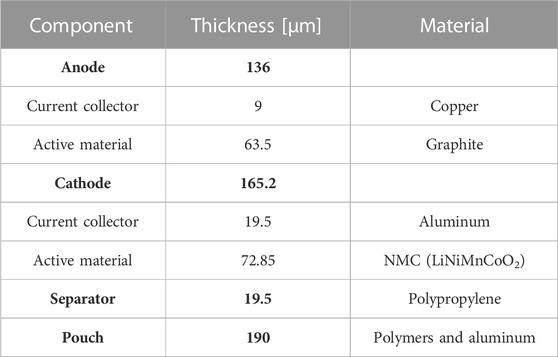
TABLE 1. Properties of the components (Kovachev et al., 2019).

The anodes consist of a current collector of copper, which is coated with a graphite-based active material on both sides. The cathodes have a core layer of aluminum covered with NMC. The separators are always in between anodes and cathodes. These are porous plies made of polypropylene. This porosity in combination with the liquid electrolyte enables the flow of ions between the electrodes.

2.2 Unit cell

A section of the described cell is used as an application example. A stack of 42 separators, 21 anodes, and 21 cathodes is utilized for this procedure. The commercial software VPS-Pam-Crash was used for modeling. The in-plane dimensions are 10 × 10 mm. The thickness of the stack results from the number of layers and the respective layer thicknesses.

This leads to an overall dimension of 10 × 10 × 7.14 mm for the section under study (Figure 1 left).

FIGURE 1

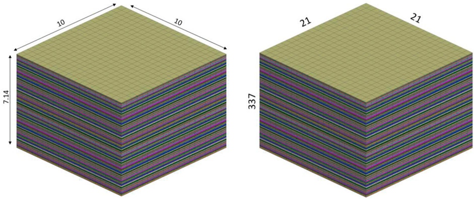
FIGURE 1. Section of lithium-ion cells under study with overall dimensions in mm (left). Number of nodes in-plane and out-of-plane (right).

As shown in Figure 1(right), the structure is discretized in the plane by 21 × 21 nodes, i.e., an element size of 0.5 mm in the plane. In the thickness direction, separators and current collectors are represented by one element each. For the discretization of the active materials, three elements are used along the thickness. Shared nodes yield the connection of the individual layers, i.e., no interlaminar slip is assumed. This results in a total of 337 nodes across the thickness. This means that the problem being investigated consists of 445,851 $DOF$ (21 × 21 × 337 × 3).

The material models of the individual layers were chosen according to their characteristic behaviors. Material parameters were established from samples extracted from a new and discharged cell (Schmid et al., 2022). The in-plane behavior of the samples was determined by tensile tests. The out-of-plane behavior was identified by compression tests. The specimen geometry for the tensile tests was 15 × 5 mm. For the compression tests, a stack of components was compressed by a flat-end impactor (D = 11 mm and R = 1 mm). For the stack of the separator, 47 layers were used, and for the electrodes, seven layers were used, resulting in a sample height of about 1 mm. For the calibration of the quasi-static material behavior, the results at the minimum test speeds were used. This was 20 mm/min for the tensile tests and 1 mm/min for the compression tests.

The section of the cell structure, as shown in Figure 1, is analyzed in three different load cases. These increases in the complexity of the load case are shown in Figure 2. In the simplest case (Figure 2A), the unit cell is only compressed in the thickness direction by 0.5 mm. All degrees of freedom of the lower nodes are locked. In the second load case, in addition to the compression in the thickness direction by 0.5 mm, a shear load in x- and y-directions is added. Therefore, the upper nodes are displaced by 0.2 mm in the x- and y-directions (Figure 2B). In the last load case, as shown in Figure 2C, in addition to the compression, the upper nodes are displaced by 0.2 mm in the y-direction to introduce a shear loading. The displacement of the right nodes by 0.2 mm generates a tension load to the structure.

FIGURE 2

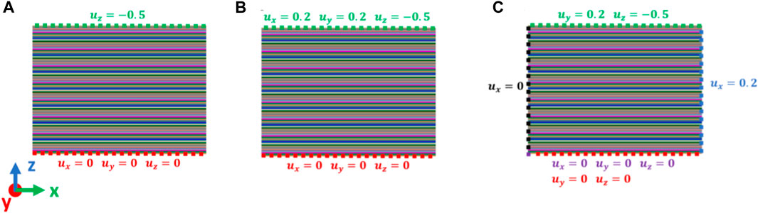
FIGURE 2. Three different load cases for the investigation of the separation of space approach: (A) compression in the thickness direction, (B) compression and shear loading of the stack, and (C) compression, shear, and in-plane tension loading.

For all three load cases, the problem is solved linearly implicitly. This allows the global system of equations to be exported. This consists of the global stiffness matrix $\mathit{K}$, the global external force vector $\mathit{F}$, and the global displacement vector $\mathit{U}$. Once the global system is assembled using the commercial solver, it can be solved quickly by applying the PGD-based separation of space approach. Python 3.8 is used for this approach. The global displacement vector $\mathit{U}$ computed via VPS is exported to compare the PGD-based solution. Moreover, an a posteriori separated approximation of $\mathit{U}$ is built via the POD to be able to compare the PGD in-plane and out-of-plane displacements.

2.3 A priori in-plane/out-of-plane model reduction based on PGD

Let us describe mathematically the unit cell and the related finite element-based simulation. For this purpose, the unit cell is represented by the three-dimensional separable domain $\mathrm{\Omega }\subset {\mathbb{R}}^3$, expressed as $\mathrm{\Omega }={\mathrm{\Omega }}_{xy}\times {\mathrm{\Omega }}_z$, where ${\mathrm{\Omega }}_{xy}\subset {\mathbb{R}}^2$ represents a two-dimensional domain and ${\mathrm{\Omega }}_z\subset \mathbb{R}$ is a one-dimensional domain. The subscripts are related to the notation used for the corresponding variables, the vector $\left(x,y\right)$ and the scalar $z$, respectively. A geometrical discretization is introduced, defining an in-plane grid ${\mathrm{\Omega }}_{xy}^h$, composed of $N_{xy}$ nodes and an out-of-plane grid ${\mathrm{\Omega }}_z^h$, of $N_z$ nodes. The three-dimensional mesh is recovered by the Cartesian product of these grids ${\mathrm{\Omega }}^h={\mathrm{\Omega }}_{xy}^h\times {\mathrm{\Omega }}_z^h$, yielding a total number of nodes $N=N_{xy}{N}_z$. For clarity, it should be noticed that the superscript $h$, as customarily used in numerical methods, just tracks a generic discrete grid defined over the domain.

Let us now introduce a 3D displacement field $\mathit{u}\left(x,y,z\right)$ of the discretised structure ${\mathrm{\Omega }}^h$, where the bold notation accounts for its components $\mathit{u}=\left(u,v,w\right)$, each one being a function of $\left(x,y,z\right)$. For notational simplicity, let us denote with $m$ the number of in-plane nodes $N_{xy}$ and $L$ with the number of layers, corresponding to the number of out-of-plane nodes $N_z$. A numerical computation (by the aid of a finite element simulation, for instance) leads to the nodal displacement, as shown in Equation (12).

$\mathbf{U}=\left(\begin{array}{c}{\mathbf{u}}_1\\ {\mathbf{u}}_2\\ ⋮\\ {\mathbf{u}}_L\end{array}\right)\in {\mathbb{R}}^{3mL\times 1}.(12)$

Here, each ${\mathbf{u}}_l$ collects the in-plane displacements at layer $l=1,\dots ,L$. Since each displacement has its own components $\left(x,y,z\right)$, it is expressed as given in in Equation (13).

${\mathbf{u}}_l={\left(u_{l,1},u_{l,2},\dots ,u_{l,m},v_{l,1},v_{l,2},\dots ,v_{l,m},w_{l,1},w_{l,2},\dots ,w_{l,m}\right)}^T\in {\mathbb{R}}^{3m\times 1}.(13)$

The numerical solution of a mechanical problem defined over $\mathrm{\Omega }$, for instance, using the finite element method, can, however, be computationally prohibitive. Indeed, when rich through-the-thickness behaviors need to be captured, a 3D finite element formulation should be employed, and a high number of degrees of freedom is often required in the thickness direction (Feng and Aymerich, 2014; Duan et al., 2020; Lin et al., 2020). Moreover, if the structure is a degenerated domain, for instance, thin structures where the size of ${\mathrm{\Omega }}_{xy}$ is much larger than ${\mathrm{\Omega }}_z$, the size of the elements shall scale with the out-of-plane mesh granularity $h_z$, to avoid highly distorted elements (poor aspect ratio). Such requirements often cause an excessively high computational complexity.

Let us consider, for instance, a full 3D finite element formulation of a static linear problem within an implicit simulation framework. This leads to the assembled system, where $\mathbf{K}\in {\mathbb{R}}^{3mL\times 3mL}$ denotes the stiffness matrix and $\mathbf{F}\in {\mathbb{R}}^{3mL\times 1},$ the nodal load vector (Eq. 14).

$\mathbf{K}\mathbf{U}=\mathbf{F}.(14)$

The numerical resolution of the linear system is an expensive task in finite element simulations with a huge number of $DOF$. Indeed, for a first remark about the complexity of a finite element simulation, the analysis of Farmaga et al. (2011) is followed. Let us denote with $C$ a positive constant, namely, the number of operations per element, and with W the (sparse) stiffness matrix bandwidth. Moreover, let $E$ be the total number of elements and $N$ the total number of nodes. The assembly of $\mathbf{K}$ and $\mathbf{F}$ is carried out by first evaluating the related contributions of a single element (so-called local quantities) and then looping over all the elements. If $C$ is the number of operations needed for the local assembly of one element, then for global assembly, this scales asymptotically as $\mathcal{O}\left(CE\right)=\mathcal{O}\left(E\right)$. This reduces to $\mathcal{O}\left(E\right)$ as constants are disregarded with asymptotic notation.

A second assembly step is required to add modifications for prescribed nodal values, whose complexity, in the worst case, amounts to $\mathcal{O}\left(NW\right)$. The solution of the system is also usually divided into two stages. The first one is reordering. For instance, when using Gaussian elimination, the matrix is transformed to an upper triangular matrix, requiring an asymptotic complexity of $\mathcal{O}\left(N{W}^2\right)$. Second, the inversion of the system scales with $\mathcal{O}\left(NW\right)$. In such a case, the total complexity scales asymptotically as $\mathcal{O}\left(N{W}^2\right)$. Since the transformation to an upper triangular matrix grows fastest, it governs the complexity, which finally scales asymptotically as $\mathcal{O}\left(N{W}^2\right)$.

Within the literature of linear algebra, numerous algorithms have been proposed to accelerate the matrix inversion stage. Most of the methods are based on matrix bandwidth reduction, adequate preconditioning, reordering, and factorizations (George and Liu, 1978; Saad, 2003; Timothy, 2006; Sybis et al., 2016; Conejero et al., 2022).

Since in this work we look for an in-plane/out-of-plane reduced-order model, the most suitable strategy for the linear system solution is that proposed in Leon et al. (2019) and Germoso et al. (2020). Such a method avoids the inversion of the full 3D system, based on enforcing an in-plane/out-of-plane separated representation in the solution, leading to a sequence of 2D and 1D systems.

Here, the a priori in-plane/out-of-plane separated representation of the algebraic system is presented Leon et al. (2019). For a better understanding, the linear system from Equation (14) can be put into the form of Equation (15).

$\left(\begin{array}{cccc}{\mathbf{K}}_{11}& {\mathbf{K}}_{12}& \cdots & {\mathbf{K}}_{1L}\\ {\mathbf{K}}_{21}& {\mathbf{K}}_{22}& \cdots & {\mathbf{K}}_{2L}\\ ⋮& ⋮& \ddots & ⋮\\ {\mathbf{K}}_{L1}& {\mathbf{K}}_{L2}& \cdots & {\mathbf{K}}_{LL}\end{array}\right)\left(\begin{array}{c}{\mathbf{u}}_1\\ {\mathbf{u}}_2\\ ⋮\\ {\mathbf{u}}_L\end{array}\right)=\left(\begin{array}{c}{\mathbf{F}}_1\\ {\mathbf{F}}_2\\ ⋮\\ {\mathbf{F}}_L\end{array}\right),$

${\mathbf{u}}_l={\left(u_{l,1},u_{l,2},\dots ,u_{l,m},v_{l,1},v_{l,2},\dots ,v_{l,m},w_{l,1},w_{l,2},\dots ,w_{l,m}\right)}^T,$

${\mathbf{F}}_l={\left(F_{l,1}^x,F_{l,2}^x,\dots ,F_{l,m}^x,F_{l,1}^y,F_{l,2}^y,\dots ,F_{l,m}^y,F_{l,1}^z,F_{l,2}^z,\dots ,F_{l,m}^z\right)}^T.(15)$

A reduced in-plane/out-of-plane form of the solution is assumed and built by means of an iterative algorithm detailed hereafter. For each layer $l=1,\dots ,L$, the separated form, as shown in Eq. 16, is enforced, where ${\mathbf{P}}^k$ denotes the $k$th in-plane mode and ${\mathbf{T}}_l^k$ denotes the $k$th out-of-plane contribution for the current layer. The product of these two functions is called a mode, with its total number $n$ in the reduced model. The symbol $\circ$ stands for the element-wise Hadamard product.

${\mathbf{u}}_l\approx {\mathbf{u}}_l^n={\displaystyle \sum _{k=1}^n}{\mathbf{P}}^k\circ {\mathbf{T}}_l^k.(16)$

2.3.1 In-plane mode definition

The in-plane mode ${\mathbf{P}}^k$ is defined by the three components of the displacement, where ${\mathcal{P}}_{•}^k$ contains the in-plane nodal values of the component $•$ (See Eq. 17).

${\mathbf{P}}^k=\left(\begin{array}{c}{\mathcal{P}}_u^k\\ {\mathcal{P}}_v^k\\ {\mathcal{P}}_w^k\end{array}\right)\in {\mathbb{R}}^{3m\times 1},$

${\mathcal{P}}_{•}^k=\left(\begin{array}{c}{P}_{•,1}^k\\ P_{•,2}^k\\ ⋮\\ P_{•,m}^k\end{array}\right)\in {\mathbb{R}}^{m\times 1}.(17)$

2.3.2 Out-of-plane mode definition

In Eq. 18, in the out-of-plane mode, at fixed layer $l$, ${\mathbf{T}}_l^k$ is expressed in a similar manner, where ${\mathcal{T}}_{•,l}^k$ contains the nodal values of the component $•$ at layer $l$, replicated for all the in-plane $DOF$ values.

${\mathbf{T}}_l^k=\left(\begin{array}{c}{\mathcal{T}}_{u,l}^k\\ {\mathcal{T}}_{v,l}^k\\ {\mathcal{T}}_{w,l}^k\end{array}\right)\in {\mathbb{R}}^{3m\times 1},$

${\mathcal{T}}_{•,l}^k=T_{•,l}^k\left(\begin{array}{c}1\\ 1\\ ⋮\\ 1\end{array}\right)=T_{•,l}^k{\mathbf{1}}_m\in {\mathbb{R}}^{m\times 1}.(18)$

2.3.3 PGD mode computation

The PGD unknown vectors are computed iteratively by means of alternating in-plane and out-of-plane problems. Let us suppose that, at the enrichment step $n$, ${\mathbf{u}}_l^{n-1}$ has already been computed. Then, the PGD solution at the current enrichment is expressed as given in Equation (19).

${\mathbf{u}}_l^n={\mathbf{u}}_l^{n-1}+{\mathbf{P}}^n\circ {\mathbf{T}}_l^n={\displaystyle \sum _{k=1}^{n-1}}{\mathbf{P}}^k\circ {\mathbf{T}}_l^k+{\mathbf{P}}^n\circ {\mathbf{T}}_l^n.(19)$

At this stage, the quantity ${\mathbf{P}}^n\circ {\mathbf{T}}_l^n$, for $l=1,\dots ,L$, is computed by means of an alternating direction strategy (ADS) up to a fixed point. This implies a further index $\left(k\right)$ to track the ADS non-linear iteration. For instance, starting from an initial guess for the out-of-plane function, the fixed-point method is as follows:

•${{\mathbf{T}}_l^n}^{\left(0\right)}assumed$

•$fork>0,untilstagnationof{{\mathbf{P}}^n}^{\left(k\right)}\circ {{\mathbf{T}}_l^n}^{\left(k\right)},do$

1. in-plane update: fix ${{\mathbf{T}}_l^n}^{\left(k-1\right)}$ and find ${{\mathbf{P}}^n}^{\left(k\right)}$,

2. out-of-plane update: fix ${{\mathbf{P}}^n}^{\left(k\right)}$ and find ${{\mathbf{T}}_l^n}^{\left(k\right)}$.

The first remark concerns the initial guess ${{\mathbf{T}}_l^n}^{\left(0\right)}$ for $l=1,\dots ,L$. As previously defined, ${\mathbf{T}}_l^n$ involves only the three unknown scalar values $T_{u,l}^n$, $T_{v,l}^n$, and $T_{w,l}^n$, which are then replicated over the in-plane grid for algorithmic reasons. This means that the out-of-plane vector to be assumed is basically the through-the-thickness kinematics of the three components $u$, $v$, and $w$, as shown in Equation (20).

${\mathbf{T}}^n={\left(\begin{array}{ccccccc}{T}_{u,1}^n& T_{v,1}^n& T_{w,1}^n& \cdots & T_{u,L}^n& T_{v,L}^n& T_{w,L}^n\end{array}\right)}^T\in {\mathbb{R}}^{3L\times 1}.(20)$

In the following section, we enter in the details of the in-plane and out-of-plane updates. For the sake of notational simplicity, the superscript $k$ of the non-linear iteration is suppressed.

2.3.4 In-plane update

By defining the diagonal matrices ${\mathbb{Z}}_l^j=diag\left({\mathbf{T}}_l^j\right)\in {\mathbb{R}}^{3m\times 3m}$, for each PGD iteration $j=1,\dots ,n$ and for each layer $l=1,\dots ,L,$ the by-layer nodal displacement is written, as in Equation (21).

${\mathbf{u}}_l^n={\displaystyle \sum _{k=1}^{n-1}}{\mathbb{Z}}_l^k{\mathbf{P}}^k+{\mathbb{Z}}_l^n{\mathbf{P}}^n.(21)$

Concatenating the matrices for all the layers, as shown in Equation (22), the total displacement approximation is expressed, as in Equation (23).

${\mathbb{T}}^j=\left(\begin{array}{c}{\mathbb{Z}}_1^j\\ ⋮\\ {\mathbb{Z}}_L^j\end{array}\right)\in {\mathbb{R}}^{3mL\times 3m},(22)$

${\mathbf{U}}^n={\mathbf{U}}^{n-1}+{\mathbb{T}}^n{\mathbf{P}}^n={\displaystyle \sum _{k=1}^{n-1}}{\mathbb{T}}^k{\mathbf{P}}^k+{\mathbb{T}}^n{\mathbf{P}}^n.(23)$

In the in-plane update, we look for the vector ${\mathbf{P}}^n$, which minimizes the current residual of the linear system, as described in Equation (24).

${\mathbf{R}}^n=\mathbf{F}-\mathbf{K}{\mathbf{U}}^n=\left(\mathbf{F}-\mathbf{K}{\mathbf{U}}^{n-1}\right)-\mathbf{K}{\mathbb{T}}^n{\mathbf{P}}^n={\mathbf{R}}^{n-1}-\mathbf{K}{\mathbb{T}}^n{\mathbf{P}}^n=\mathbf{0}.(24)$

Rearranging the terms and pre-multiplying the equation by ${{\mathbb{T}}^n}^T$, we obtain the reduced system to be solved, which is shown in Equation (25).

$\left({{\mathbb{T}}^n}^T\mathbf{K}{\mathbb{T}}^n\right){\mathbf{P}}^n={{\mathbb{T}}^n}^T{\mathbf{R}}^{n-1}.(25)$

Such a system scales with the number of in-plane nodes $m$ since ${{\mathbb{T}}^n}^T\mathbf{K}{\mathbb{T}}^n\in {\mathbb{R}}^{3m\times 3m}$, for an asymptotic complexity of $\mathcal{O}\left(m\right)$.

2.3.5 Out-of-plane update

In this step, the unknown vector is ${\mathbf{T}}^n$, which can explicitly appear in the expression of the current displacement ${\mathbf{U}}^n$, after defining suitable matrices in the same fashion of the in-plane update.

To this purpose, let us define the diagonal matrices ${\mathbb{P}}^j=diag\left({\mathbf{P}}^j\right)\in {\mathbb{R}}^{3m\times 3m}$, for each PGD iteration $j=1,\dots ,n$, and the in-plane replicating matrix $\mathbf{C}$, as shown in Equation (26).

$\mathbf{C}=\left(\begin{array}{ccc}{\mathbf{1}}_m& {\mathbf{0}}_m& {\mathbf{0}}_m\\ {\mathbf{0}}_m& {\mathbf{1}}_m& {\mathbf{0}}_m\\ {\mathbf{0}}_m& {\mathbf{0}}_m& {\mathbf{1}}_m\end{array}\right)\in {\mathbb{R}}^{3m\times 3}.(26)$

Here, ${\mathbf{1}}_m\in {\mathbb{R}}^{m\times 1}$ and ${\mathbf{0}}_m\in {\mathbb{R}}^{m\times 1}$ have entries all equal to 1 and 0, respectively. In such a way, the current displacement at layer $l$ is expressed, as given in Equation (27).

${\mathbf{u}}_l^n={\displaystyle \sum _{k=1}^n}{\mathbb{P}}^k\mathbf{C}\left(\begin{array}{c}{T}_{u,l}^k\\ T_{v,l}^k\\ T_{w,l}^k\end{array}\right).(27)$

The total through-the-thickness displacement is obtained by introducing the block diagonal matrix (Equation (28)), accounting for all the $L$ layers where $\mathbf{0}\in {\mathbb{R}}^{3m\times 3}$ has only zero entries. This yields the global displacement, as shown in Equation (29).

${\mathfrak{P}}^k=\left(\begin{array}{cccc}{\mathbb{P}}^k\mathbf{C}& \mathbf{0}& \dots & \mathbf{0}\\ \mathbf{0}& \ddots & \ddots & ⋮\\ ⋮& \ddots & \ddots & \mathbf{0}\\ \mathbf{0}& \dots & \mathbf{0}& {\mathbb{P}}^k\mathbf{C}\end{array}\right)\in {\mathbb{R}}^{3mL\times 3L},(28)$

${\mathbf{U}}^n={\mathbf{U}}^{n-1}+{\mathfrak{P}}^n{\mathbf{T}}^n.(29)$

This is enforced in the current global residual to obtain the out-of-plane problem, which is shown in Equation (30).

${\mathbf{R}}^n=\mathbf{F}-\mathbf{K}{\mathbf{U}}^n=\left(\mathbf{F}-\mathbf{K}{\mathbf{U}}^{n-1}\right)-\mathbf{K}{\mathfrak{P}}^n{\mathbf{T}}^n={\mathbf{R}}^{n-1}-\mathbf{K}{\mathfrak{P}}^n{\mathbf{T}}^n=\mathbf{0}.(30)$

Rearranging the terms and pre-multiplying the equation by ${{\mathfrak{P}}^n}^T$, we obtain the reduced system to be solved, which is shown in Equation (31).

$\left({{\mathfrak{P}}^n}^T\mathbf{K}{\mathfrak{P}}^n\right){\mathbf{T}}^n={{\mathfrak{P}}^n}^T{\mathbf{R}}^{n-1}.(31)$

Such a system scales with the number of out-of-plane layers since ${{\mathfrak{P}}^n}^T\mathbf{K}{\mathfrak{P}}^n\in {\mathbb{R}}^{3L\times 3L}$, for an asymptotic complexity of $\mathcal{O}\left(L\right)$.

This procedure is performed until a defined number of iteration $K$ is reached or the result is not changing anymore. This means that the deviation error $\xi$ of two consecutive iterations is below a defined limit ${\xi }_{limit}$. To evaluate this, the Frobenius norm ${‖•‖}_F$ is used, as shown in Equation (32).

$\xi =\frac{{‖{\mathfrak{P}}^n{\mathbf{T}}^n-{{\mathbb{T}}^n\mathbf{P}}^n‖}_F}{{‖{{\mathbb{T}}^n\mathbf{P}}^n‖}_F}.(32)$

It is worth noting that the full 3D system involving the matrix $\mathbf{K}\in {\mathbb{R}}^{3mL\times 3mL}$, whose asymptotic complexity scales as $\mathcal{O}\left(mL\right)$, is never inverted. The complexity of each PGD enrichment is now written asymptotically as $\mathcal{O}\left(K\left(m+L\right)\right)$, where $K$ is the number of fixed-point iterations. The complexity of each PGD mode $k=1,\dots ,n$ is now asymptotically written as $\mathcal{O}\left(K\left(m+L\right)\right)$, where $K$ is the number of fixed-point iterations. This means that the total complexity can be written as a function of $n,K,m,L$ as $\mathcal{O}\left(nK\left(m+L\right)\right)$.

The method presented here is used to solve the three linear problems shown in Figure 2. Both the computation time and the resulting error are used to evaluate the efficiency. As a reference, the classical solution of the problem is used by inverting the stiffness matrix $\mathbf{K}$. As a measure of the resulting error, again the Frobenius norm is used, which is shown in Equation (33).

$\epsilon =\frac{{‖{\mathit{U}}^{inv}-{\mathit{U}}^{PGD}‖}_F}{{‖{\mathit{U}}^{PGD}‖}_F}.(33)$

2.4 A posteriori in-plane/out-of-plane model reduction based on POD

For the sake of comparison of the PGD results, an in-plane/out-of-plane model of the displacement $\mathbf{U}$ (expressed in Eq. 12) can be obtained a posteriori inspired by the POD (Antoulas, 2005; Volkwein, 2013). The displacements are collected by components splitting ${\mathbf{u}}_l$ of Equation (13) in the vectors, which are given in Equation (34).

$\left.\begin{array}{c}{{\mathbf{u}}_l^x=\left(u_{l,1},u_{l,2},\dots ,u_{l,m}\right)}^T\\ {\mathbf{u}}_l^y={\left(v_{l,1},v_{l,2},\dots ,v_{l,m}\right)}^T\\ {\mathbf{u}}_l^z={\left(w_{l,1},w_{l,2},\dots ,w_{l,m}\right)}^T\end{array}\right\}\in {\mathbb{R}}^{m\times 1}.(34)$

The by-component matrices, as shown in Equation (35), are binding such vectors by columns.

$\left.\begin{array}{c}{\mathbf{U}}^x=\left(\begin{array}{cccc}{\mathbf{u}}_1^x& {\mathbf{u}}_2^x& \cdots & {\mathbf{u}}_L^x\end{array}\right)\\ {\mathbf{U}}^y=\left(\begin{array}{cccc}{\mathbf{u}}_1^y& {\mathbf{u}}_2^y& \cdots & {\mathbf{u}}_L^y\end{array}\right)\\ {\mathbf{U}}^z=\left(\begin{array}{cccc}{\mathbf{u}}_1^z& {\mathbf{u}}_2^z& \cdots & {\mathbf{u}}_L^z\end{array}\right)\end{array}\right\}\in {\mathbb{R}}^{m\times L}.(35)$

The POD applies to each one of these matrices in the standard form of the singular value decomposition (SVD). For instance, considering ${\mathbf{U}}^x$, the SVD is expressed, as given in Equation (36).

${\mathbf{U}}^x={\mathit{P}}_u{\mathrm{\Sigma }}_u{\mathit{T}}_u^T.(36)$

Where ${\mathit{P}}_u\in {\mathbb{R}}^{m\times m}$ contains the eigenvectors of ${{\mathbf{U}}^x}^T{\mathbf{U}}^x$, ${\mathit{T}}_u\in {\mathbb{R}}^{L\times L}$ contains the eigenvectors of ${\mathbf{U}}^x{{\mathbf{U}}^x}^T$ and ${\mathrm{\Sigma }}_u\in {\mathbb{R}}^{m\times L}$ is the matrix storing the singular values $\mathrm{\sigma }$. The reduced singular value decomposition of rank $r>0$ finds instead the separated approximation where the matrices with superscript $r$ are obtained considering only the first $r$ eigenvectors, as in Equation (37).

${\mathbf{U}}^x\approx {\mathbf{U}}_r^x={\mathit{P}}_u^r{\mathrm{\Sigma }}_u^r{\mathit{T}}_u^r{}^T.(37)$

In the literature of the POD, the first $r$ eigenvectors are also referred to principal modes, and in this case, they give a reduced in-plane/out-of-plane separated representation of the displacement field.

It shall be noticed that this POD-based model reduction requires the full knowledge of the displacement field, coming from the full inversion of the system in Equation (14). This entails all the computational drawbacks previously discussed.

3 Results

3.1 Material calibration

The unit cell consists of five different material models:

• Separator

• Anode—current collector

• Anode—active material

• Cathode—current collector

• Cathode—active material

For the calibration of the respective material models, the results of tensile tests and compression tests were used, as discussed by Schmid et al. (2022). In Figure 3, the simulations are compared with the mean results of the experiments.

FIGURE 3

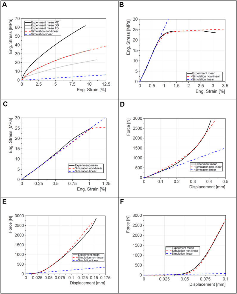
FIGURE 3. Comparison between simulation and experiments of the component tests. Tensile tests: (A) separator, (B) anode, and (C) cathode; compression tests: (D) separator, (E) anode, and (F) cathode.

Since a linearized problem is dealt with in the following section, two different simulation variants were carried out. The red curves show the results of the quasi-static non-linear simulations. The results of the static linear versions are shown in blue.

Subplots a–c show the comparison of simulation and experiments of the tensile tests. The parameters of all material models are shown in Table 2. Anodes and cathodes behaved approximately isotropically. Therefore, an isotropic elastic–plastic material model was chosen for the current collectors. It is assumed that the active material has no significant effect on the in-plane behavior. This was taken into account by a tensile cutoff (TCO) stress of ${1.010}^{-5}$ GPa.

TABLE 2

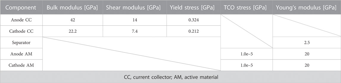
TABLE 2. Parameters of different material models.

In contrast to the electrodes, the separator has anisotropic in-plane behavior. Therefore, three experimental mean curves are shown in Figure 3A. The samples utilized in the machine direction (MD) behave more stiffly than those utilized in the transverse direction (TD). The averaged curve of the diagonal direction (DD) lies in between. With the non-linear foam model chosen for the separator, this anisotropy cannot be taken into account. Therefore, the results of the diagonal direction were used for the calibration of the tensile behavior. In the linearized calculation, the initial slope of the compression curve is also used as the tensile stiffness in this material model. This results in deviations between the red and blue curves even in the range of small strains. However, it is evident that a distinction is made between the tension and compression phases in the case of a non-linear solution. This leads to much better results despite the unchanged material model.

Figures 3D–F show the results of the compression tests. The results are used to calibrate the compression properties of the active materials and the separator. The same material model (non-linear foam) was used for the active materials of the anode and cathode as for the separator. Again, the non-linear simulation results are shown in red, and the linearized results are in blue.

3.2 Application of proper generalized decomposition

Non-linear material models were used for all components. Nevertheless, the application of the presented approach is shown on a linearized problem—as the first step—for three different load cases. This was performed to avoid an intrusive approach. Thus, a deeper insight into the behavior and results of the method is possible. All three load cases, as shown in Figure 2, were solved with the described procedure. The applied deformation is considered small enough to perform a static linear calculation. The results are shown in Figures 4–7. A value of ${10}^{-6}$ was chosen as the limit value ${\xi }_{limit}$ for the alternating direction strategy. If this value is not achieved in 50 iterations, the process is terminated anyway, and the next mode is calculated. In all three cases, 10 modes are used.

FIGURE 4

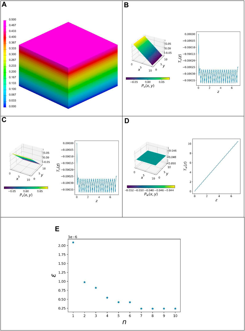
FIGURE 4. Results of load case I: (A) quasi-static linear FEM solution (displacement norm), (B) first mode u-direction, (C) first mode v-direction, (D) first mode w-direction, and (E) resulting error over the number of modes.

Figure 4 shows the results of the first load case. Here, the unit cell is compressed in the thickness direction. The fringe plot of the displacement norm of the linear static calculation using VPS-Pam-Crash is shown in Figure 4A. This shows a maximum of 0.5 mm and occurs at the upper nodes where the Dirichlet boundary conditions are applied.

Figures 4B and C show the results of the first mode. Each mode is composed of three components (u-, v-, and w-components). These are, in turn, divided into an in-plane function $\mathbf{P}$ and an out-of-plane function $\mathbf{T}$. Accordingly, $\mathbf{P}$ is dependent on the in-plane position (x- and y-coordinates), and $\mathbf{T}$ is the function of the z-coordinate. Figure 4B shows the function for the u-component (displacement in the x-direction). Here, we can observe the characteristic shape, which is marked by oscillations. This area of the curve has 42 deflections, which is consistent with the number of electrodes. These are due to the current collectors, which also expand in-plane as a result of the Poisson’s effect during transverse compression. The same characteristic curve is observed for the v-component (displacement in the y-direction). The w-component (displacement in the z-direction) does not show such pronounced oscillations. Here, only different displacements of the layers in the thickness direction are evident in the $\mathbf{T}$ function. From the in-plane function $\mathbf{P}$, it is observed that all areas are compressed equally when viewed over the x–y plane.

The computing time of the commercial solver VPS-Pam-Crash is used to compare the efficiency of the PGD method with respect to classical strategies. The linear static calculation is carried out in parallel (DMP 16 cores). This comparison shows that on average, only about half the computing time of the industrial solution is needed to calculate the first PGD mode. In addition, the PGD routine in Python is not optimized in terms of computing time, unlike the solver.

The resulting error $\epsilon$ over the number of modes used is shown in Figure 4E. This shows that the first mode is already sufficient to achieve a deviation of only ${2.110}^{-6}$. With the following modes, this value can be minimized to ${0.2510}^{-6}$.

Figure 5 shows the results obtained with PGD compared to the POD results from the procedure illustrated in Section 2.3. The left half shows the three normalized components of the first PGD mode, and the right half shows the same components with POD. For the POD components, the result of the classical FEM solution was used as the basis for the data. (Eqs 34–37). The first 10 singular values are shown in Figure 5(bottom). Therefore, the ratio of a singular value and the sum of all are used. Again, it can be seen that the first mode is sufficient to obtain a sufficiently good approximation of the solution. Comparing all three components of the first mode, it is noticeable that no significant deviations are apparent between the PGD and the POD results.

FIGURE 5

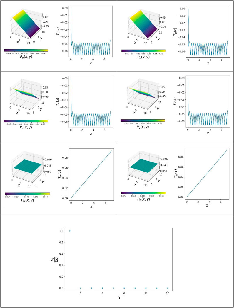
FIGURE 5. Comparison of PGD and POD for load case I: PGD (left) and POD (right). Resulting singular values over the number of modes (bottom).

The results of the second load case are shown in Figure 6. According to Figure 2B, in this case, both compressions in the thickness direction and shear in x- and y-directions are applied. The results calculated using VPS-Pam-Crash are shown in Figure 6A. The displacement norm here is a maximum of 0.575 mm. This again concerns the top node layer.

FIGURE 6

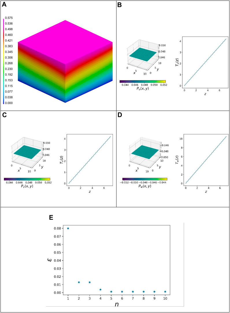
FIGURE 6. Results of load case II: (A) quasi-static linear FEM solution (displacement norm), (B) first mode u-direction, (C) first mode v-direction, (D) first mode w-direction, and (E) resulting error over the number of modes.

The three functions for the u-, v-, and w-components are shown in subplots b and c. For all three components, the in-plane function $\mathbf{P}$ assumes a constant value. The out-of-plane component $\mathbf{T}$ has a linear course from a global point of view. Locally, however, it is characterized by different stiffnesses of the individual layers. These lead to minor oscillations. This affects all three components.

The resulting error $\epsilon$, which describes the deviations between these two solutions, is shown in Figure 6E over the number of modes used. Already with the first mode, the error $\epsilon$ of about 0.08 can be achieved. With the following two modes, this value can be reduced to about 0.014. With the following extensions, a minimum value of 0.005 is achieved.

The results of the third load case are shown in Figure 7. These correspond to the boundary conditions in Figure 2C. This is the most complex of the three load cases. The unit cell is compressed more in the thickness direction than in the previous cases. In addition to a shear load, a tensile load is applied in the plane. The fringe plot of the high dimensional solution is shown in Figure 7A. The maximum displacement norm here is 0.575 mm. This value is present at the front upper edge.

FIGURE 7

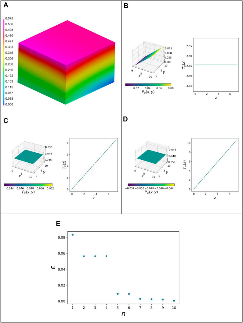
FIGURE 7. Results of load case III: (A) quasi-static linear FEM solution (displacement norm), (B) first mode u-direction, (C) first mode v-direction, (D) first mode w-direction, and (E) resulting error over the number of modes.

The u-component of the first mode is shown in subplot 7b. This is the component that determines the in-plane displacement and represents the in-plane tensile load. Here, it is noticeable that the out-of-plane function $\mathbf{T}$ has a constant value across the thickness. The in-plane function $\mathbf{P}$ is also constant along the y-coordinate. The x-direction appears linear only in the in-plane function. The v-component of the first mode is shown in Figure 7C. The in-plane function $\mathbf{P}$ is constant along both coordinates. The out-of-plane function $\mathbf{T}$ has a stepped curve over the z-coordinate. The functions of the w-component (Figure 7D) show a similar characteristic shape. The in-plane function $\mathbf{P}$ is constant here as well but with a negative value. The out-of-plane function $\mathit{T}$ also has a stepped curve over the thickness. This corresponds to the basic pattern that is expected from the described boundary conditions, which is also evident from the fringe plot in Figure 7A.

The deviation of the reduced solution using PGD from the solution of the commercial solver is shown in Figure 7E over the number of modes in use. With the first mode, a deviation of 0.08 can already be achieved. With the three further modes, this value is reduced to 0.06. By using all 10 modes, the resulting error can be minimized to 0.004.

4 Conclusion

In this work, an alternative modeling and simulation framework is proposed in the field of lithium-ion batteries, which are sensible toward out-of-plane loading.

From one side, the study provides a useful in-plane/out-of-plane characterization of the mechanical behavior, preventing simplification hypotheses coming from shell-based formulations. On the other side, the methodology circumvents fully solid-based solutions, which are unaffordable for large-scale systems involving extremely thin structures. Moreover, an additional faced challenge is the minimal intrusiveness of the proposed procedure, which should be easily integrated into commercial FEA software.

The algorithm exploits standard FEA software for the model definition, structure discretization, and finite element assembly. Afterward, the assembled system is tackled by means of the PGD method, implemented as an external plug-in. This reorders the original system in a layer-wise manner and enforces a separated representation of the solution into in-plane and out-of-plane components. The unknown increasing components are calculated via an iterative algorithm based on an alternating direction strategy (ADS), highly reducing the number of degrees of freedom involved in the subproblems. The product of these two components is called a mode. By stringing together several modes, the quality of the result is improved.

Since, in implicit simulations, system inversion is a really computationally demanding task; explicit computations are often preferred in industry, at the price of losing accuracy and verifying time-stepping requirements. However, including the PGD-based system solution in implicit computations appears as an appealing alternative. Indeed, the total complexity of the PGD algorithm is expressed as $\mathcal{O}\left(nK\left(m+L\right)\right)$, while that of classical methods, as $\mathcal{O}\left(3mL\right)$. Since $n$ and $K$ are usually small (in the present study, $n\le 10$ and $K<10$ allow an accurate enough solution) and $mL\gg m+L$, the PGD complexity is much lower than classical inversion, making the algorithm particularly attractive.

The method is exemplified over three different load cases of a linearized static problem defined for a lithium-ion cell. The model is defined using the industrial software application VPS-Pam-Crash, and the structure is discretized using solid elements, obtaining a laminate with a large number of degrees of freedom along the thickness.

The results show that the deviation decreases with the number of modes used. For example, in load case I, one mode is sufficient to achieve a deviation of only ${2.110}^{-6}$. For the other load cases, which are more complex, several modes are needed to achieve a sufficiently small deviation below 1%. Thus, the load influences how many modes are required.

By comparing PGD and POD, it was shown that almost the same results were obtained. The main advantage of the PGD method presented here is that no a priori database is required, while the POD-reduced model is built only after solving the full system.

The computing time of the commercial FEA software application VPS-Pam-Crash (parallel computing) is compared with the needed time of the PGD routine. It has been shown that on average, it takes about the same time to calculate two modes using Python as it does for the classical FEM solution in VPS-Pam-Crash. However, it should be noted that the PGD implementation is performed using Python without code parallelization and optimizations, which will be addressed in further studies.

5 Outlook

In this work, the application was shown on a static linear problem. However, the more common problems are cases with non-linear behavior due to the material models. The application of the presented procedure to non-linear problems with bigger deformations is part of the current research. At least a semi-intrusive approach is required to enable the iterative solution (Equations 9–11) using commercial software. A comparison between the modified Newton–Raphson procedure, the original Newton–Raphson method, and the one with PGD would be interesting. The implementation of this PGD-based model order reduction approach would also allow a better comparison of the computational time. By implementing it in a commercial solver, a fair comparison can be achieved since both solution variants are carried out in the same environment.

The performance of quasi-static non-linear calculations would also increase the quality of the material models. In particular, for the separator (non-linear foam), static linear calculations do not subdivide into compressive and tensile stiffnesses. However, for the representation of the in-plane anisotropy, a fundamentally different material model must be used.

Additional potential in terms of computing time can be generated by optimizing the PGD solution strategy. The alternating direction strategy is used to calculate a mode. For this, an assumption must be made in the first step (initial guess). The choice of this assumption has an influence on how many iterations have to be carried out to calculate the two functions $\mathbf{T}$ and $\mathbf{P}$. In the current work, a uniform initial guess was made. It can be assumed that an advanced selection strategy shows potential to increase the efficiency.

First, a possible embedding or linking of this method with common crash simulations—which mainly use explicit time integration—is carried out by sequential or simultaneous co-simulation (Esgandari and Olatunbosun, 2015; Hu and Zhong, 2019). Next, the envelope (pouch) of the lithium-ion cell is explicitly simulated. This simulation also includes contact modeling of the cell environment. The jellyroll is modeled in detail and solved time-efficiently using PGD in a parallel implicit calculation. This makes it possible to explicitly simulate the structure of the cell environment without suffering from the critical time step of the fine discretization of the cell structure.

Data availability statement

The original contributions presented in the study are included in the article/Supplementary Material; further inquiries can be directed to the corresponding authors.

Author contributions

Writing–original draft: AS and AP. Conceptualization: AP, AS, CE, VC, FC, and FF. Data curation: AS, AP, MR, and VC. Methodology: AP, AS, CE, FC, and FF. Validation: AS, MR, and MZ. Visualization: AP and AS. Writing–review and editing: AS, AP, CE, FF, MZ, VC, MR, and FC. Supervision: CE, FF, and FC. Project administration: CE, FF, and FC. All authors contributed to the article and approved the submitted version.

Funding

This work was conducted during the realization of the project SafeLIB (grant agreement no. 882506) with data from the previous project SafeBattery as a collaboration of the Vehicle Safety Institute of Graz University of Technology and Arts et Métiers ParisTech (Paris Campus, PIMM Lab). SafeBattery was funded within the framework of COMET—Competence Centers for Excellent Technologies and by the Province of Styria, as well as the Styrian Business Promotion Agency SFG. The follow-up SafeLIB has additionally been funded by the Province of Upper Austria. Both projects are administered by the Austrian Research Promotion Agency (FFG).

Acknowledgments

The authors would like to thank the mentioned agencies and the cooperating companies. Additionally, the authors acknowledge the support of the ESI Group through its research chair CREATE-ID at ENSAM ParisTech supported by the TU Graz Open Access Publishing Fund.

Conflict of interest

MZ and FC are employed at ESI Group; AP and VC are employed at ESI Group Chair.

The remaining authors declare that the research was conducted in the absence of any commercial or financial relationships that could be construed as a potential conflict of interest.

Publisher’s note

All claims expressed in this article are solely those of the authors and do not necessarily represent those of their affiliated organizations, or those of the publisher, the editors and the reviewers. Any product that may be evaluated in this article, or claim that may be made by its manufacturer, is not guaranteed or endorsed by the publisher.

References

Antoulas, A. C. (2005). Approximation of large-scale dynamical systems. Philadelphia, PA, United States: Society for Industrial and Applied Mathematics.

Google Scholar

Arief Budiman, B., Rahardian, S., Saputro, A., Hidayat, A., Pulung Nurprasetio, I., and Sambegoro, P. (2022). Structural integrity of lithium-ion pouch battery subjected to three-point bending. Eng. Fail. Anal. 138, 106307. doi:10.1016/j.engfailanal.2022.106307

CrossRef Full Text | Google Scholar

Beaumont, R., Masters, I., Das, A., Lucas, S., Thanikachalam, A., and Williams, D. (2021). Methodology for Methodology for Developing a Macro Finite Element Model of Lithium-Ion Pouch Cells for Predicting Mechanical Behaviour under Multiple Loading Conditionseveloping a macro finite element model of lithium-ion pouch cells for predicting mechanical behaviour under multiple loading conditions. Energies 14 (7), 1921. doi:10.3390/en14071921

CrossRef Full Text | Google Scholar

Bognet, B., Leygue, A., and Chinesta, F. (2014). Separated representations of 3D elastic solutions in shell geometries. Adv. Simul. Eng. 1 (4), 4. doi:10.1186/2213-7467-1-4

CrossRef Full Text | Google Scholar

Breitfuss, C., Sinz, W., Feist, F., Gstrein, G., Lichtenegger, B., Knauder, C., et al. (2013). A ‘Microscopic’ Structural Mechanics FE Model of a Lithium-Ion Pouch Cell for Quasi-Static Load Casesicroscopic’ structural mechanics FE model of a lithium-ion pouch cell for quasi-static load cases. SAE Int. J. Passeng. Cars - Mech. Syst. 6 (2), 1044–1054. doi:10.4271/2013-01-1519

CrossRef Full Text | Google Scholar

Budde-Meiwes, H., Drillkens, J., Lunz, B., Muennix, J., Rothgang, S., Kowal, J., et al. (2013). A review of current automotive battery technology and future prospects. Proc. Institution Mech. Eng. Part D J. Automob. Eng. 227 (5), 761–776. doi:10.1177/0954407013485567

CrossRef Full Text | Google Scholar

Chen, H., Buston, J. E., Gill, J., Howard, D., Williams, R. C., Rao Vendra, C. M., et al. (2020). An experimental study on thermal runaway characteristics of lithium-ion batteries with high specific energy and prediction of heat release rate. J. Power Sources 472, 228585. doi:10.1016/j.jpowsour.2020.228585

CrossRef Full Text | Google Scholar

Conejero, J. A., Falco, A., and Mora-Jimenez, M. (2022). Structure and approximation properties of Laplacian-like matrices. Results Math. 78. doi:10.21203/rs.3.rs-2099815/v1

CrossRef Full Text | Google Scholar

Duan, M., Yue, Z., and Song, Q. (2020). Investigation of damage to thick composite laminates under low-velocity impact and frequency-sweep vibration loading conditions. Adv. Mech. Eng. 12 (10), 168781402096504. doi:10.1177/1687814020965042

CrossRef Full Text | Google Scholar

Esgandari, M., and Olatunbosun, O. (2015). Implicit–explicit co-simulation of brake noise. Finite Elem. Analysis Des. 99, 16–23. doi:10.1016/j.finel.2015.01.011

CrossRef Full Text | Google Scholar

Farmaga, I., Shmigelskyi, P., Spiewak, P., and Ciupinski, L. “Evaluation of computational complexity of finite element analysis,” in Proceedings of the 2011 11th International Conference The Experience of Designing and Application of CAD Systems in Microelectronics (CADSM), Polyana, Ukraine, February 2011, 213–214.

Google Scholar

Feng, D., and Aymerich, F. (2014). Finite element modelling of damage induced by low-velocity impact on composite laminates. Compos. Struct. 108, 161–171. doi:10.1016/j.compstruct.2013.09.004

CrossRef Full Text | Google Scholar

George, A., and Liu, J. W. H. (1978).Algorithms for matrix partitioning and the numerical solution of finite element systems Philadelphia, PA, United States: Society for Industrial and Applied Mathematics.

Google Scholar

Germoso, C., Quaranta, G., Duval, J. L., and Chinesta, F. (2020). Non-Non-Intrusive In-Plane-Out-of-Plane Separated Representation in 3D Parametric Elastodynamicsntrusive in-plane-out-of-plane separated representation in 3D parametric elastodynamics. Computation 8 (3), 78. doi:10.3390/computation8030078

CrossRef Full Text | Google Scholar

Ghnatios, C., Barasinski, A., and Chinesta, F. (2022). On the On the High-Resolution Discretization of the Maxwell Equations in a Composite Tape and the Heating Effects Induced by the Dielectric Lossesigh-resolution discretization of the maxwell equations in a composite tape and the heating effects induced by the dielectric losses. Computation 10 (2), 24. doi:10.3390/computation10020024

CrossRef Full Text | Google Scholar

Ghnatios, C., El Haber, G., Duval, J.-L., Ziane, M., and Chinesta, F. (2021). Artificial intelligence based space reduction of structural models. ESAFORM 2021. doi:10.25518/esaform21.2004

CrossRef Full Text | Google Scholar

Gilaki, M., and Avdeev, I. (2016). Impact modeling of cylindrical lithium-ion battery cells: impact modeling of cylindrical lithium-ion battery cells: a heterogeneous approach heterogeneous approach. J. Power Sources 328, 443–451. doi:10.1016/j.jpowsour.2016.08.034

CrossRef Full Text | Google Scholar

Goutaudier, D., Berthe, L., and Chinesta, F. (2022). Exploring space separation techniques for 3D elastic waves simulations. Comput. Mech. 69 (5), 1147–1163. doi:10.1007/s00466-021-02134-x

CrossRef Full Text | Google Scholar

Guo, G., Long, B., Cheng, B., Zhou, S., Xu, P., and Cao, B. (2010). Three-dimensional thermal finite element modeling of lithium-ion battery in thermal abuse application. J. Power Sources 195 (8), 2393–2398. doi:10.1016/j.jpowsour.2009.10.090

CrossRef Full Text | Google Scholar

Hu, H., and Zhong, Z. (2019). Explicit–Explicit–Implicit Co-Simulation Techniques for Dynamic Responses of a Passenger Car on Arbitrary Road Surfacesmplicit Co-simulation techniques for dynamic responses of a passenger car on arbitrary road surfaces. Engineering 5 (6), 1171–1178. doi:10.1016/j.eng.2019.09.003

CrossRef Full Text | Google Scholar

Kazemzadeh-Parsi, M. J., Ammar, A., Duval, J. L., and Chinesta, F. (2021b). Enhanced parametric shape descriptions in PGD-based space separated representations. Adv. Model. Simul. Eng. Sci. 8 (1), 23. doi:10.1186/s40323-021-00208-2

CrossRef Full Text | Google Scholar

Kazemzadeh-Parsi, M.-J., Ammar, A., and Chinesta, F. (2023). Parametric Parametric Analysis of Thick FGM Plates Based on 3D Thermo-Elasticity Theory: a Proper Generalized Decomposition Approachnalysis of thick fgm plates based on 3D thermo-elasticity theory: a proper generalized decomposition approach. Mater. (Basel, Switz. 16, 1753–4. doi:10.3390/ma16041753

CrossRef Full Text | Google Scholar

Kazemzadeh-Parsi, M.-J., Chinesta, F., and Ammar, A. (2021a). Proper Proper Generalized Decomposition for Parametric Study and Material Distribution Design of Multi-Directional Functionally Graded Plates Based on 3D Elasticity Solutioneneralized decomposition for parametric study and material distribution design of multi-directional functionally graded plates based on 3D elasticity solution. Mater. (Basel, Switz. 14, 6660–21. doi:10.3390/ma14216660

CrossRef Full Text | Google Scholar

Kazemzadeh-Parsi, M. J., Ammar, A., and Chinesta, F. (2022). Domain decomposition involving subdomain separable space representations for solving parametric problems in complex geometries. Adv. Model. Simul. Eng. Sci. 9 (1), 2. doi:10.1186/s40323-022-00216-w

CrossRef Full Text | Google Scholar

Kermani, G., Keshavarzi, M. M., and Sahraei, E. (2021). Deformation of lithium-ion batteries under axial loading: analytical model and Representative Volume Element. Energy Rep. 7, 2849–2861. doi:10.1016/j.egyr.2021.05.015

CrossRef Full Text | Google Scholar

Kim, G.-H., Pesaran, A., and Spotnitz, R. (2007). A three-dimensional thermal abuse model for lithium-ion cells. J. Power Sources 170 (2), 476–489. doi:10.1016/j.jpowsour.2007.04.018

CrossRef Full Text | Google Scholar

Kisters, T., Sahraei, E., and Wierzbicki, T. (2017). Dynamic impact tests on lithium-ion cells. Int. J. Impact Eng. 108, 205–216. doi:10.1016/j.ijimpeng.2017.04.025

CrossRef Full Text | Google Scholar

Klein, B. (2015). Fem: grundlagen und Anwendungen der Finite-Element-Methode im Maschinen-und Fahrzeugbau. Wiesbaden, Germany: Springer Fachmedien Wiesbaden.

Google Scholar

Kovachev, , Schröttner, , Gstrein, , Aiello, , Hanzu, , Wilkening, , et al. (2019). Analytical Analytical Dissection of an Automotive Li-Ion Pouch Cellissection of an automotive Li-ion pouch cell. Batteries 5 (4), 67. doi:10.3390/batteries5040067

CrossRef Full Text | Google Scholar

Lee, S., and Park, S. S. (2012). Atomistic Atomistic Simulation Study of Monoclinic Li₃V₂(PO₄)₃ as a Cathode Material for Lithium Ion Battery: structure, Defect Chemistry, Lithium Ion Transport Pathway, and Dynamicsimulation study of monoclinic Li3V2(PO4)3 as a cathode material for lithium ion battery: structure, defect chemistry, lithium ion transport pathway, and dynamics. J. Phys. Chem. C 116 (48), 25190–25197. doi:10.1021/jp306105g

CrossRef Full Text | Google Scholar

Leon, A., Mueller, S., de Luca, P., Said, R., Duval, J.-L., and Chinesta, F. (2019). Non-intrusive proper generalized decomposition involving space and parameters: non-intrusive proper generalized decomposition involving space and parameters: application to the mechanical modeling of 3D woven fabricspplication to the mechanical modeling of 3D woven fabrics. Adv. Model. Simul. Eng. Sci. 6 (1), 13. doi:10.1186/s40323-019-0137-8

CrossRef Full Text | Google Scholar

Lin, S., Thorsson, S. I., and Waas, A. M. (2020). Predicting the low velocity impact damage of a quasi-isotropic laminate using EST. Compos. Struct. 251, 112530. doi:10.1016/j.compstruct.2020.112530

CrossRef Full Text | Google Scholar

Quaranta, G., Bognet, B., Ibañez, R., Tramecon, A., Haug, E., and Chinesta, F. (2018). A new hybrid explicit/implicit in-plane-out-of-plane separated representation for the solution of dynamic problems defined in plate-like domains. Comput. Struct. 210, 135–144. doi:10.1016/j.compstruc.2018.05.001

CrossRef Full Text | Google Scholar

Quaranta, G., Ziane, M., Haug, E., Duval, J.-L., and Chinesta, F. (2019). A minimally-intrusive fully 3D separated plate formulation in computational structural mechanics. Adv. Model. Simul. Eng. Sci. 6 (1), 11. doi:10.1186/s40323-019-0135-x

CrossRef Full Text | Google Scholar

Raffler, M., Sinz, W., Erker, S., Brunnsteiner, B., and Ellersdorfer, C. (2022). Influence of loading rate and out of plane direction dependence on deformation and electro-mechanical failure behavior of a lithium-ion pouch cell. J. Energy Storage 56, 105906. doi:10.1016/j.est.2022.105906

CrossRef Full Text | Google Scholar

Reynolds, C. D., Slater, P. R., Hare, S. D., Simmons, M. J., and Kendrick, E. (2021). A review of metrology in lithium-ion electrode coating processes. Mater. Des. 209, 109971. doi:10.1016/j.matdes.2021.109971

CrossRef Full Text | Google Scholar

Saad, Y. (2003). Iterative methods for sparse linear systems. Philadelphia, PA, United States: Society for Industrial and Applied Mathematics. doi:10.1137/1.9780898718003

CrossRef Full Text | Google Scholar

Sahraei, E., Bosco, E., Dixon, B., and Lai, B. (2016). Microscale failure mechanisms leading to internal short circuit in Li-ion batteries under complex loading scenarios. J. Power Sources 319, 56–65. doi:10.1016/j.jpowsour.2016.04.005

CrossRef Full Text | Google Scholar

Sahraei, E., Campbell, J., and Wierzbicki, T. (2012). Modeling and short circuit detection of 18650 Li-ion cells under mechanical abuse conditions. J. Power Sources 220, 360–372. doi:10.1016/j.jpowsour.2012.07.057

CrossRef Full Text | Google Scholar

Schmid, A., Ellersdorfer, C., Raffler, M., Karajan, N., and Feist, F. (2022). An efficient detailed layer model for prediction of separator damage in a Li-Ion pouch cell exposed to transverse compression. SSRN. doi:10.2139/ssrn.4273879

CrossRef Full Text | Google Scholar

Sonnberger, P., Behmer, M., Böhler, E., and Breitfuss, C. (2022). A hybrid approach to derive macro- and meso-mechanic cell models for vibrational investigations of lithium-ion pouch cells. J. Energy Storage 49, 104060. doi:10.1016/j.est.2022.104060

CrossRef Full Text | Google Scholar

Sybis, M., Smoczkiewicz-Wojciechowska, A., and Szymczak-Graczyk, A. (2016). Impact of matrix inversion on the complexity of the finite element method. Sci. Transp. Prog. Bull. Dnipropetrovsk Natl. Univ. Railw. Transp. 62, 190–199. doi:10.15802/stp2016/67358

CrossRef Full Text | Google Scholar

Tang, L., Zhang, J., and Cheng, P. (2017). Homogenized modeling methodology for 18650 lithium-ion battery module under large deformation. PloS one 12 (7), e0181882. doi:10.1371/journal.pone.0181882

PubMed Abstract | CrossRef Full Text | Google Scholar

Tertrais, H., Ibañez, R., Barasinski, A., Ghnatios, C., and Chinesta, F. (2019). On the Proper Generalized Decomposition applied to microwave processes involving multilayered components. Math. Comput. Simul. 156, 347–363. doi:10.1016/j.matcom.2018.09.008

CrossRef Full Text | Google Scholar

Timothy, A. D. (2006). Direct methods for sparse linear systems (fundamentals of algorithms 2). Philadelphia, PA, United States: Society for Industrial and Applied Mathematics.

Google Scholar

Üçel, İ. B., and Gudmundson, P. (2022). A statistical RVE model for effective mechanical properties and contact forces in lithium-ion porous electrodes. Int. J. Solids Struct. 244-245, 111602. doi:10.1016/j.ijsolstr.2022.111602

CrossRef Full Text | Google Scholar

Väyrynen, A., and Salminen, J. (2012). Lithium ion battery production. J. Chem. Thermodyn. 46, 80–85. doi:10.1016/j.jct.2011.09.005

CrossRef Full Text | Google Scholar

Volkwein, S. (2013). “Proper orthogonal decomposition: theory and reduced-order modelling,” in Lecture notes (Konstanz, Germany: University of Konstanz).

Google Scholar

Waldmann, T., Iturrondobeitia, A., Kasper, M., Ghanbari, N., Aguesse, F., Bekaert, E., et al. (2016). Review—Review—Post-Mortem Analysis of Aged Lithium-Ion Batteries: disassembly Methodology and Physico-Chemical Analysis Techniquesost-mortem analysis of aged lithium-ion batteries: disassembly methodology and physico-chemical analysis techniques. J. Electrochem. Soc. 163 (10), A2149–A2164. doi:10.1149/2.1211609jes

CrossRef Full Text | Google Scholar

Wang, L., Yin, S., and Xu, J. (2019). A detailed computational model for cylindrical lithium-ion batteries under mechanical loading: from cell deformation to short-circuit onset. J. Power Sources 413, 284–292. doi:10.1016/j.jpowsour.2018.12.059

CrossRef Full Text | Google Scholar

Wierzbicki, T., and Sahraei, E. (2013). Homogenized mechanical properties for the jellyroll of cylindrical Lithium-ion cells. J. Power Sources 241, 467–476. doi:10.1016/j.jpowsour.2013.04.135

CrossRef Full Text | Google Scholar

Yang, K.-H. (2018). Basic finite element method and analysis as applied to injury biomechanics. Cambridge, Massachusetts, United States: Academic Press, 377–378.

Google Scholar

Zhao, Y., Stein, P., Bai, Y., Al-Siraj, M., Yang, Y., and Xu, B.-X. (2019). A review on modeling of electro-chemo-mechanics in lithium-ion batteries. J. Power Sources 413, 259–283. doi:10.1016/j.jpowsour.2018.12.011

CrossRef Full Text | Google Scholar

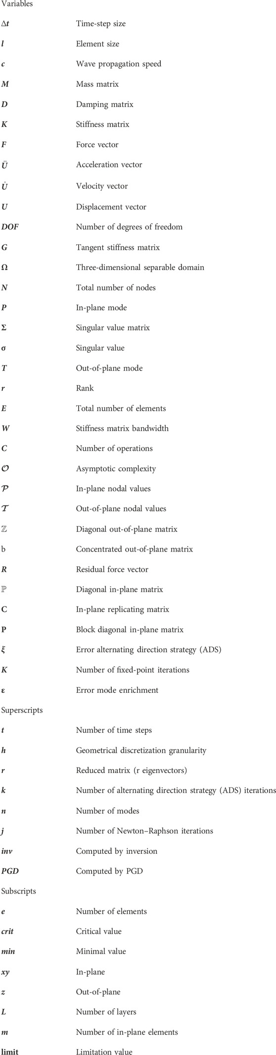
Nomenclature