Modeling a domain wall network in BiFeO3 with stochastic geometry and entropy-based similarity measure

1 Introduction

Ferroelectric domain walls (DWs) are the boundaries between two regions with differently oriented electrical polarization on a crystal structure and can be one or two atoms wide (Jia et al., 2007). They show enhanced conductivity compared to that of the domains (Seidel et al., 2009; Catalan et al., 2012; Meier et al., 2012), and their density and topological complexity can be modulated by the choice of the substrate and the system dimensions (Vlooswijk et al., 2007; Nesterov et al., 2013; Feigl et al., 2014), e.g., the film thickness. Their non-trivial electronic and transport properties have been demonstrated to be suitable for new applications of domain wall nanoelectronics (Catalan et al., 2012; Meier and Selbach, 2022). DWs can also provide memristive features (Maksymovych et al., 2011; Chen et al., 2023; Liu et al., 2023). In particular, both DWs’ enhanced conductivity with respect to domains (Chiu et al., 2011; Farokhipoor and Noheda, 2011; 2012) and DWs’ memristive behavior (Rieck et al., 2022) have been observed in as-grown self-assembled ferroelectric–ferroelastic DW networks where conduction is “lateral,” i.e., the charge flows parallel to the surface through the DW network from wall to wall.

Thus, self-assembled DW networks are potential candidates for neuromorphic information processing. Neuromorphic computing has emerged in recent years as a possible solution to the ever-increasing demand for computational power. The paradigm was ignited by Mead (2020), and it aims to the emulation of the brain learning capabilities that arise from the collective dynamics of a large number of interacting elements. Nowadays, new memristive technologies have been proposed and effectively used to mimic the brain’s ability to encode information and synapse-like dynamics in materio (Indiveri et al., 2013; Christensen et al., 2022). Wiring together memristive devices enables the realization of cross-bar arrays for the fast and energy-efficient hardware implementation of vector-matrix multiplications (Mannocci et al., 2023), which is one of the most expensive computational steps in modern neural network models in artificial intelligence. Nevertheless, the full potential of biological neural systems is achieved through the interplay between their complex topological structures and the functional dynamics of several elements evolving on them (Suárez et al., 2021). Self-assembled memristive networks of nano-objects, such as nanoparticle self-assembled networks (Bose et al., 2017; Mambretti et al., 2022; Profumo et al., 2023) or nanowire networks (Hochstetter et al., 2021; Milano et al., 2021; Montano et al., 2022), have been proposed as potential candidates to emulate the structure–function interplay of biological systems. Because ferroelastic DW formation is due to the release of an epitaxial strain imposed by the substrate, they cannot be easily moved, removed, or created with an electric field. Thus, this kind of system might provide a more robust plastic connectivity structure between input leads located on the substrate compared to other self-assembled neuromorphic systems. Self-assembled neuromorphic networks are complex systems, and unraveling their characteristics along with their potential for information processing requires an analysis of both their functional, i.e., dynamical, and structural properties. The diversity of the response of a complex system can be determined only by the coupling between both components (Ghavasieh and De Domenico, 2023). The network anatomy has a vital impact on a complete description of a complex system as the structure affects the dynamics that cope with that topology at different time scales (Pastor-Satorras and Vespignani, 2001; Strogatz, 2001; Moreno and Pacheco, 2004) and ultimately affect the function. In some cases, as for a memristive network, the reverse is also true. The dynamics can also possibly affect the structure of a system, where, in this specific case, we mean the distribution of conductance. In this regard, such coupling has been investigated in the case of other self-assembled materials with intricate structures (Loeffler et al., 2020; Milano et al., 2022) through simulation. Even though the ultimate task is to reassemble topology and function in a complete mathematical description (Caravelli et al., 2023; Caravelli et al., 2021), because of the non-linearity of some systems, e.g., the memristive dynamics, simulations are still required to shed light on their functional behavior, as shown in our previous work (Cipollini and Schomaker, 2023).

The structural connectivity can be accessed experimentally by modern imaging techniques, such as optical microscopy, conductive atomic force microscopy (cAFM), electron backscatter diffraction, or X-ray diffraction microscopy. Unfortunately, high-quality microstructural images are particularly time-consuming and costly in terms of laboratory equipment. Furthermore, it is difficult to cover all possible “states of interest” as either the image measurements might not disclose the degree of statistical homogeneity desired or the parameter space might be too large to be sampled within a reasonable time. Thus, solely relying on experimental imaging techniques for obtaining the necessary microstructural data is insufficient, and synthetic models for materials provide a practical alternative to these issues.

In this work, we focus on the structural connectivity of the DW network in BiFeO₃ (BFO) thin films that show lateral conduction. Under the framework of complex network theory together with tessellation methods from stochastic geometry, this study defines a two-dimensional generative model for the network structure of ferroelectric–ferroelastic DWs in BFO thin films. The DW network structure was experimentally accessible, thanks to the conductive atomic force microscopy (cAFM) imaging technique, and manual annotation of nodes and edges on the image was undertaken to build a dataset of DW networks (see Section 2.1).

1.1 Complex network theory

Complex systems, both artificial and natural, find an abstract yet powerful representation through network structures, which are defined by nodes interconnected by edges. A complex network theory provides a robust framework for modeling and understanding the structural and functional organization of such complex systems when encoded into the mathematical form of graphs (Newman, 2010). Specifically, in the context of self-assembled neuromorphic structures (e.g., DWs in crystal structures and nanowire networks), when complemented with a model for the dynamical memristive properties of the edges, it facilitates the understanding of the transport properties of these systems.

Complex network theory is becoming increasingly popular because of its vast applicability; nevertheless, several questions remain open. For instance, questions such as how to measure the distance between two graphs and, consequently, how to measure the likelihood of the network model parameters with respect to the observed empirical network are important in the context of networks. In other words, it is important to know how much information is gained when we try to describe the empirical network structure derived from data with a prescribed model. When the task is to find the best set of model parameters to reproduce some empirical networks, according to the model, maximization of the log-likelihood is very well-suited (Cimini et al., 2019). Maximum-likelihood methods on graphs aim to compare the ability of different models to describe empirical networks, that is, to optimize model parameters to fit soft constraints, which are quantities of interest. Hence, an ensemble of graphs is partially defined by the graph model, and maximizing the (log-) likelihood completes such a definition, which results in fixing the constraints to be equal, on average, to what is measured on the empirical networks. The model selection problem and inference of parameters are thus solved by constraining a subset of local or global features of the network structure on the proposed model to be, on average, equal to the empirical network, e.g., degree correlations, degree distribution, and clustering coefficients. A canonical ensemble of networks is thus defined, according to which the same probability is assigned to networks that satisfy the same set of constraints. Nevertheless, the caveat is in the imposition of some global or local features that do not necessarily capture the intrinsically multi-scale structure of heterogeneous networks as a whole (Cimini et al., 2019; Nicolini et al., 2020).

The work of Domenico and Biamonte (2016) recently proposed von Neumann entropy for networks to condense the description of the multi-scale network structure in a single quantity. They extended the information-theoretic framework of quantum mechanics to define the entropy of complex networks by focusing on how the information diffuses over the network topology. A density matrix, which typically encodes mixed states in quantum physics (Feynman, 1998), is used to encode the network structure. The definition of a density matrix for networks enables the extension of the von Neumann entropy to complex networks computed as the Shannon entropy of its eigenvalues.

1.1.1 Spectral entropy and diffusion in networks

When studying information spreading (Domenico and Biamonte, 2016) and the identification of core structures in heterogeneous systems (Villegas et al., 2022), diffusion processes are essential. The graph Laplacian governs diffusion in networks (Masuda et al., 2017), and its eigenvalue spectrum encodes many relevant topological properties of the graph (Anderson and Morley, 1985; Estrada, 2011). Let us consider an undirected and unweighted simple network G(V, E), where |V| = N and |E| = L are the number of nodes and links, respectively. The network combinatorial Laplacian is defined as $\widehat{L}=\widehat{D}-\widehat{A}$, where $\widehat{D}$ and $\widehat{A}$ are the diagonal matrix of the node degrees and the adjacency matrix, respectively. Given an initial state of the network encoding the amount of information in one or more nodes, $\underline{s}(0)$, the state at time τ is given by $\underline{s}(\tau )=e^{-\tau \widehat{L}}\underline{s}(0)$, where $\widehat{K}=e^{-\tau \widehat{L}}$ is the network propagator. The ensemble of accessible diffusive states at time τ is defined through the network propagator by the density matrix (Domenico and Biamonte, 2016; Nicolini et al., 2018; Ghavasieh et al., 2020):

$\widehat{\rho }=\frac{e^{-\tau \widehat{L}}}{Z},(1)$

where $\widehat{\rho }(\tau )$ can be interpreted as the canonical density operator in statistical physics. Each element ρ_ij represents the normalized amount of information transferred in a diffusion process between nodes i and j at time τ, where ρ_ij takes into account all possible topological pathways between the two nodes and assigns smaller weights to longer ones (Feynman, 1998; Villegas et al., 2022). The partition function $Z=\mathrm{Tr}[\widehat{K}]={\sum }_{i=1}^N{e}^{-\tau {\lambda }_i(\widehat{L})}$ is a function of the eigenvalues, λ_i, of the Laplacian and is proportional to the average return probability of a random walker to be back in its initial location at time τ. The object $\widehat{\rho }$ is a positive semi-definite and Hermitian matrix whose trace sums to unity, allowing its eigenvalues to be interpreted as probabilities. Therefore, the von Neumann entropy is defined as follows:

$S\left(\widehat{\rho }\left(\tau \right)\right)=-{\displaystyle \sum _{i=1}^N}{\mu }_i\left(\tau \right)\log {\mu }_i\left(\tau \right),(2)$

where ${\{{\mu }_i(\tau )\}}_i^N$ is the set of $\widehat{\rho }(\tau )$ eigenvalues that are related to the set of Laplacian matrix eigenvalues through ${\mu }_i(\tau )=e^{-\tau {\lambda }_i}/Z$. The entropy $S(\widehat{\rho }(\tau ))$ is a function of the normalized time τ and is bounded between [log  C, log  N], where C is the number of connected components and N is the number of nodes. The entropy S, as a function of τ, reflects the entropic phase transition of information propagation over the network (Villegas et al., 2022), as illustrated in Figure 1. Specifically, for a connected network, for τ → 0, S(τ) = log  N, it reflects the segregated heterogeneous phase where information diffuses from the single nodes to their local neighborhood; meanwhile, for τ → ∞, S(τ) = 0, the diffusion is governed by the smallest non-zero eigenvalue of the Laplacian, associated with the so-called Fiedler eigenvector, reflecting the homogeneous phase where information has propagated all over the network. Thus, intuitively, we can use the parameter τ in the von Neumann entropy (Eq. 2) to resolve the network topological structures at different structural scales, leveraging on the time evolution. We briefly mention that the analogy to second-order phase transitions is robust, and the specific heat can be defined and used to access the intrinsic temporal diffusion scales of the network. We refer to Villegas et al. (2023) for a more extensive explanation.Within the proposed framework, Domenico and Biamonte (2016) demonstrated the use of spectral entropy to define a distance between networks, the von Neumann relative entropy:

$S\left(\widehat{\rho }\mid \widehat{\sigma }\right)=\mathrm{Tr}\left[\widehat{\rho }\left(\log \widehat{\rho }-\log \widehat{\sigma }\right)\right],(3)$

where $\widehat{\rho }$ and $\widehat{\sigma }$ are network density matrices. This quantity describes the Kullback–Leibler divergence between two graphs, and its minimization is equivalent to maximizing the log-likelihood of the density matrix $\widehat{\sigma }$ describing the density matrix $\widehat{\rho }$. Nevertheless, to compute this quantity, both networks need to be of the same size, which is the case for networks of the canonical ensemble, but it is not suitable for our case, as is discussed in Section 2.3.

FIGURE 1

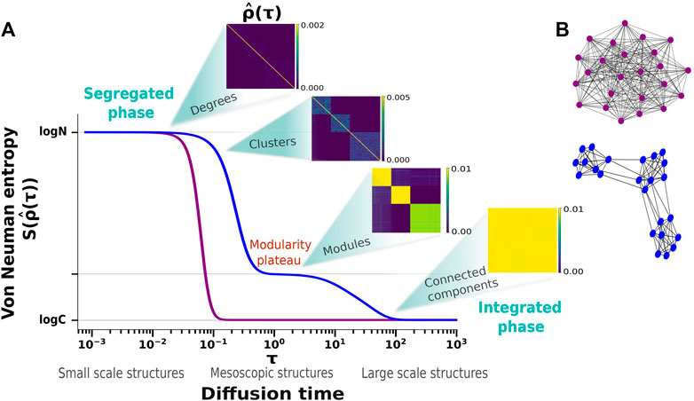
FIGURE 1. (A) Von Neumann entropy, S, as a function of the diffusion time, τ, for two exemplary networks with analogous topological features to those depicted in panel (B): in blue a stochastic block model network exhibiting tripartite modular structure, and in purple a Erdös-Rényi random network with the same number of nodes of the blue one. Graphs depicted in (B) have only illustration purpose. For small τ ∼ 0, both networks exhibit the maximum spectral entropy value log  N, where N is the number of nodes, reflecting the segregated phase. For τ → ∞, the spectral entropy converges to log  C, where C is the number of connected components, thus reflecting the integrated phase. For intermediate values of τ, the Erdös-Rényi network shows a single critical scale at which the network transitions from the segregated to the integrated phase, depicting the lack of any sign of scale-invariance in the topological structure. On the contrary, the blue network exhibits two critical resolution scales in the entropic transition. At smaller τ, information initially diffuses within the modules, afterwards a second slower diffusion between the modules completes the transition to the integrated phase. Between the two resolution scales, a plateau resolves the mesoscale properties of the network. The plateau height is associated with the modularity of the network, while its position on the horizontal axis is related to the edge density of the network. The insets show the density matrix, ρ, at different diffusion times, τ, as the entropic transition takes place along the blue curve. The tripartite modular structure of the network is shown by the emergence of the three blocks in the density matrix. Adapted from Nicolini et al. (2020) and Villegas et al. (2022).

2 Materials and methods

2.1 Data and ground truth networks

Data used in this work are from Rieck et al. (2022), and we refer to the original article for details on the experimental apparatus and experimental methods used to grow the BFO and produce the cAFM data used in this work. Here, we summarize the main points. The BFO thin films of 55-nm thickness are deposited by pulsed laser deposition (PLD) on TiO₂-terminated (100) SrTiO₃ (STO) single-crystal substrates. cAFM measurements are performed using the conductive tip of an AFM as the top electrode. For these measurements, the sample has no bottom electrode, and thus, conductivity is lateral from wall to wall. The conduction map is shown in Figure 2A and exhibits a dense and well-interconnected DW network of higher conductivity compared to the domains.

FIGURE 2

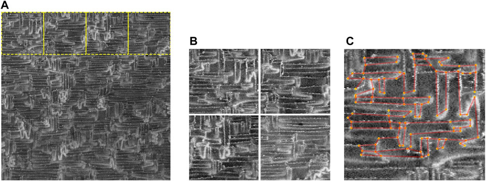
FIGURE 2. (A) Conduction map of 55-nm-thick BFO thin film from Rieck et al. (2022). A dense DW network of higher conductivity compared to the domains is revealed from the cAFM measurements. Conduction is from wall to wall. Sample size is 5 × 5 μm. Brighter regions correspond to 9-pA currents. (B) Four exemplary crops of physical linear size 1.25 μm and 128-pixel-linear size corresponding to the yellow dashed squares in (A). Panel (C) shows an example of manual graph annotation of the crop corresponding to the top-left corner of (A). Only the largest connected component is depicted. Nodes (yellow dots) are located at DW intersections. Edges (red continuous lines) connect two nodes and coincide with DWs or a part of them. DWs that continue out of the crop are not included in the annotation. More annotated crops are displayed in Supplementary Figure S1A.

The method proposed in this work is data-driven; thus, it requires a supply of a dataset of ground truth DW networks as a reference. For this purpose, the sample is cropped in 25 square patches of physical linear size 1.25 μm and 128 × 128 pixel size, as shown in Figures 2A, B. Grid-like segmentation results in 16 crops, and the 9 other crops are taken by displacing the grid-like cropping of half the linear size of the crops both on the $\widehat{y}$ and $\widehat{x}$ axes. Each crop is manually annotated with a specifically designed Python-written tool with a simple graphical user interface (GUI). Nodes are defined and manually placed in locations where DWs intersect. Edges are created by connecting two nodes such that each edge coincides with a DW or a part of it. Only DW structures that are fully contained in each single crop are included in the dataset, and DWs whose start/end/intersection is not visible in the crop are not annotated. In conclusion, from the 25 crops, we obtain a dataset of 25 DW graph-encoded networks. Importantly, after the manual annotation, the largest connected component is selected to be included in the DW network dataset. Importantly, the rules chosen for the identification of nodes and edges in the manual annotation of the experimental samples are in accordance with the automatic network extraction method applied to the synthetic samples that we discuss in Section 2.2.2, as is visually illustrated in Supplementary Figure S1.

2.2 Model

2.2.1 Voronoi tessellation

Tessellation is a class of mathematical models that divides space into non-overlapping cells (domains) that has proven to be a useful framework for models with realistic grain shapes in bulk ceramics and ferroelectric thin films in order to investigate the microstructures of materials and the structure–property relationships (Anand, 2012; Šedivý et al., 2016). This type of idealized mathematical description comes at the cost of the physical description of the underlying processes driving the formation and growth of the material. Nevertheless, in contrast to physics-based models, the geometrical approaches are less computationally demanding. To approximate the formation of a configuration of domains and walls of a given sample of the ferroelastic–ferroelectric BFO film, we need to account for both the growth and competition of distinct domains and DWs during the formation process as the material seeks to find the most stable and energetically favorable configuration under given conditions, e.g., the epitaxial strain imposed by the substrate cut, the density of domain walls due to the substrate thickness, and temperature (Catalan et al., 2012). These two key features are both available in the Voronoi scheme, where randomly displaced centroidal seeds compete with other seeds to grow and form a homogeneous region of influence. This is akin to a region of homogeneous electric polarization stochastically formed during the ferroelastic–ferroelectric film formation process. As a consequence, separating boundaries between homogeneous (polarization) regions appear both in the Voronoi-proxy process and in the physical formation process of BFO thin films, indicating the Voronoi tessellation as a natural modeling solution for mimicking the emergence of the interconnected DW network structure. The formation of a given structure of domains and DWs both in the BFO sample and in the Voronoi sample is the result of an optimization process trying to minimize either the free energy (Kittel, 1946; Landau and Lifshitz, 1992), in the case of the BFO, or a distance function, in the case of the Voronoi process. Nevertheless, in this work, we do not seek any further analogy than those discussed, but rather, we use the Voronoi process as an inductive bias over the generation of topological structures in our samples, with some control parameters acting as effective parameters gathering the overall condition under which the physical sample was grown.

We use the Voronoi tessellation to create pixel-based instances of BFO synthetic samples from which the network, in the form of graph, is subsequently extracted. Thus, the Voronoi tessellation can be regarded as the inductive bias imposed on our graph generation process. Given a set $\mathbf{P}={\{{\bar{P}}_i\}}_{i=1}^n$ of seed points on a domain $\mathbf{D}\in {\mathbb{R}}^2$, the Voronoi diagram divides the plane into convex Voronoi regions $\mathbf{V}(\mathbf{P})={\{V_i\}}_{i=1}^n$ such that

$V_i=\left\{\bar{x}\in \mathbf{D}|\Vert \bar{x}-{\bar{P}}_i\Vert \le \Vert \bar{x}-{\bar{P}}_j\Vert ,\forall j\ne i\right\}.(4)$

A Voronoi tessellation is considered centroidal when the center of mass, ${\bar{C}}_i$, of the Voronoi domains is such that ${\bar{C}}_i={\bar{P}}_i\forall i$. Given an arbitrary set of seed points, there is no guarantee that the resulting Voronoi tessellation will be centroidal. Nevertheless, given a pristine set of points, it is possible to iteratively converge toward a centroidal tessellation. We use the relaxing scheme proposed by Lloyd (1982). The process starts with computing the Voronoi diagram of an initial uniform distribution of n points ${\bar{P}}_i$ displaced over the plane. The centroids are also computed. Then, the seed points ${\bar{P}}_i$ of each region are moved to the corresponding centroids ${\bar{C}}_i$, and Voronoi regions are generated again. The algorithm stops when the maximum distance between the seed points and centroids is less than an arbitrary value. The Voronoi tessellation is a distance-based method, which means that, based on the distance metric that is used to compute the tessellation, several types of patterns can be realized (Chen et al., 2019). As an example, if a L₁-metric (Manhattan distance) is used, the Voronoi domains will converge toward a pattern of squares rotated at 45° (Efros and Leung, 1999), while the generated Voronoi region will be close to a regular hexagon if a L₂-metric distance is used. In this work, the Chebyshev distance with an axial scale is used:

$d_{\beta }\left({\bar{x}}^{\left(i\right)},{\bar{x}}^{\left(j\right)}\right)=\max \left(\beta |x_0^{\left(i\right)}-x_0^{\left(j\right)}|,\frac{1}{\beta }|x_1^{\left(i\right)}-x_1^{\left(j\right)}|\right),(5)$

where ${\bar{x}}^{(i)}=(x_0^{(i)},x_1^{(i)})$ and β is the scale factor. Rectangle-shaped Voronoi regions are generated with this metric (Chen et al., 2019).

To produce complex shapes resembling the structure of the BFO sample in Figure 2, each seed point is associated with either a vertically or horizontally axial-scaled Chebyshev distance with the probability p. The Voronoi obtained is an improper Voronoi tessellation as the domains are not convex. Moreover, as can be observed in Figure 3, the introduction of both vertically and horizontally scaled domains potentially leads to domains clashing into each other and thus creating fractured domains. In conclusion, the resulting tessellation is dependent on three parameters: the number of seed points n, the Chebyshev distance axial scale β, and the probability, p, of a domain along either the vertical or horizontal direction. Intuitively, the number of seed points governs the density of the domains and DWs, the axial scale influences the elongation of the domains and the DWs, and the probability p governs the fraction of horizontal and vertical domains together with the fraction of fractured domains and complex shapes. In the next sections, we will not refer to the number of points, n, but rather to the linear density of points, d≔n/l, where l = 128 is the linear pixel size of our samples.

FIGURE 3

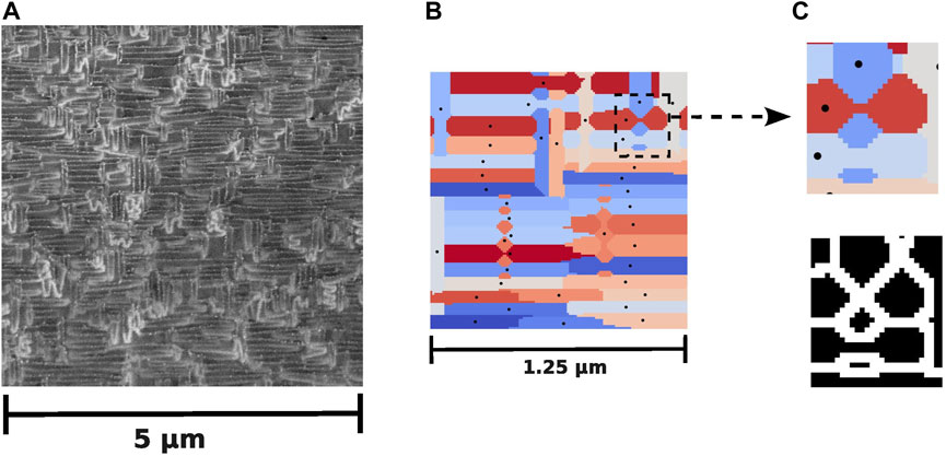
FIGURE 3. (A) BFO sample and its scale. (B) Tessellation result after 20 iterations generated with the parameters illustrated in Table 1. The seeds are indicated by black dots. The sample is of 128-pixel-linear size corresponding to 1.25 μm in physical units (see the bar at the bottom). (C) Zoomed-in view of the synthetic Voronoi sample visually illustrating the emergence of fractured domains due to the introduction of the two types of axially scaled domains, both before and after the domain border detection, as described in section 2.2.2. Note that images in panels (B, C) are rotated by 90° to the right.

2.2.2 Automatic conversion from a pixel-based to graph-based data sample

We are not interested in the domains produced by the tessellation method, which are analogous to the polarization domains in the BFO, but in the boundaries that naturally arise between the Voronoi regions that in our scheme are analogous to the DWs in the BFO. Our focus is on the network properties of the DWs in the BFO thin film, and we ultimately aim at synthetic data in a graph-based representation. To extract the DW network structures from the tessellation sample, we developed an automatic tool. A detailed description of the automatic network extraction tool can be found in Section 1 of the Supplementary Material. Here, we give a schematic description of the steps involved.

1 Synthetic Voronoi samples of pixel size 128 × 128 are generated from n seed points uniformly distributed on the 2D plane, each associated with an axial scaling of β in either the vertical or horizontal direction with probability p.

2 Walls between distinct Voronoi domains are detected with the Sobel filter (Kanopoulos et al., 1988). The output image is then binarized: all non-zero values are set to one, and the remaining pixels are left zero.

3 Automated network extraction is undertaken through the following steps:

a Nodes for the graph representation are detected through the junction detection algorithm (He et al., 2015).

b Edges for the graph representation are detected with the module from the NEFI tool (Dirnberger et al., 2015).

c Nodes that are closer to each other than $ϵ\le \sqrt{2}$ are merged.

The procedure results in both pixel-based and the respective graph-based samples of the synthetic DW network, as shown in Figure 4. See Supplementary Figure S1B for more examples of automatically extracted networks from the Voronoi samples.

FIGURE 4

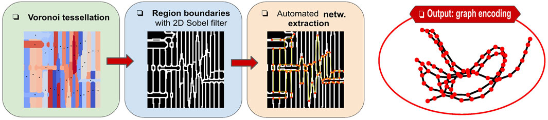
FIGURE 4. Illustration of the introduced pipeline to generate a synthetic DW network sample. We begin by generating a tessellation sample from n seed points randomly displaced over the sample of size 128 × 128 pixels. The boundaries between different tessellation domains are detected by means of the Sobel filter and the binarization step. Then, automated network extraction is undertaken over the binary image. This method results in synthetic DW networks on a pixel-level basis, along with their corresponding graph-based representations. The Voronoi sample, the binary image, and its automatically annotated counterpart depicted in this figure are generated with parameters in Table 1.

2.3 Fitting the network structure

A distance measure between networks follows the definition of the network density matrix and the spectral entropy (Domenico and Biamonte, 2016). Specifically, Domenico and Biamonte (2016) defined the Kullback–Leibler divergence (also called relative entropy) between networks and showed that it is proportional to the negative log-likelihood function. A maximum log-likelihood approach can then be used to estimate the model parameters that maximize the likelihood of reproducing the empirical samples, as previously discussed in Section 1.1.1. The procedure results in constraining the generated networks to have, on average, the same Laplacian spectrum as the empirical networks. Within the pipeline proposed in this work, the number of nodes in the network, N, cannot be held fixed; thus, any analogy to the canonical ensemble should be considered with caution (see Section 1.1). Furthermore, the relative entropy between two networks defined in this ensemble necessitates the same number of nodes to be calculated, unlike in our pipeline, where the number of nodes fluctuates. Nevertheless, while using the Voronoi tessellation to produce the pixel-based data is analogous to imposing an inductive bias on our generation model, the use of the eigenvalue spectrum of the diffusion propagator to fit the model can be interpreted as constraining the diffusion modes available in the generated networks to those of the empirical networks. Moreover, the Laplacian spectrum, on which the propagator spectrum depends, encloses several topological properties of graphs that are closely related to the conductive properties of networks (Ho et al., 1975; Klein and Randić, 1993; Ellens et al., 2011).

For what concerns this work, we directly use the spectral entropy curves to proxy the distance between the generated graphs and their desired counterpart. We estimate the optimal parameters for the tessellation-based generative model by minimization of the sum of squared error (SSE) between the empirical and synthetic spectral entropy curves in Eq. 6. The search for the optimal parameters is carried out by a standard gradient-free genetic algorithm (Mitchell, 1998) implemented by the PyGAD library (Gad, 2021) as no gradient can be easily identified in our method. During each generation, 96 ensembles, each defined by a set of parameters for the Voronoi generation, are sampled, generating 25 network instances per ensemble. The average spectral entropy measured over the 25 samples is used to estimate the fitness value per ensemble, according to Eq. 6. The selection of parents for the mating pool of size 24 is carried out by rank selection. Elitism is not used; thus, at each generation, step offsprings originate exclusively from the selected parents. An offspring mutation probability of 0.1 is set for all genes, giving each gene of each offspring a 10% likelihood to undergo a random mutation.

The fitness function maximized by the genetic algorithm is defined as

$f={\displaystyle \sum _{\tau }}{\left(<S\left(\tau \right)>-<S{\left(\tau \right)>}_{\mathit{dataset}}\right)}^{-2},(6)$

where $<S{(\tau )>}_{\mathit{dataset}}$ and $<S(\tau )>$ are the average spectral entropy measured for the ground truth networks set and the set of generated networks, respectively. Convergence of the genetic optimization method is illustrated in Figures 5A,B.

FIGURE 5

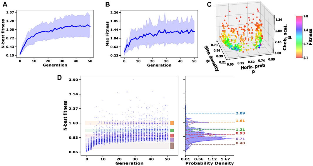
FIGURE 5. Optimization of parameters. Each network ensemble is defined by a fixed set of parameters, {d, p, β}, and the ensemble fitness value is calculated by sampling 25 networks. Panels (A) and (B) depict the average fitness value of the 10 best ensembles per generation and the maximum fitness value per generation, respectively. Each curve is averaged over 15 independent optimization processes. The shaded areas represent the standard deviation. In (C), each point represents one of the 10 best ensembles per generation collected across the 15 independent optimization processes, thus leading to a total of 10 × 50 × 15 = 7500 points. Colors represent the estimated ensemble fitness (red = low and blue/purple = high). We observe a symmetric displacement of points with respect to the horizontal probability parameter, p, and two symmetric attractors in the parameter space: p* ≃ 2 and p = 1 − p*. Both attractors lead to comparable fitness values demonstrating invariance under rotation in our method. (D) Ten best fitness values per generation collected across the 15 independent optimization processes, shown on the left, and the distribution of the same values illustrated by the histogram, shown on the right. Fitness values are clustered with the Gaussian mixture model. For each Gaussian, the mean parameter, μ, is written on the right, while the standard deviation is illustrated by the colored vertical bar and the shaded areas spanning the optimization history. It should be noted that the y-axis is shared between the two plots and that only fitness values corresponding to parameter solutions where p ≤ 0.5 are included. To obtain the ensemble parameters shown in Table 1, we average those ensemble parameters that are included in one standard deviation from the Gaussian with μ = 1.61.

The 10 best ensemble parameters per generation collected across the 15 independent optimization processes are plotted in Figure 5C. We observe the symmetric disposition of points with respect to the axis p = 0.5, thus identifying two attractors in the ensemble parameter space. The color code indicates comparable fitness values for points on either one of the two sides of the symmetry axis. Thus, solutions with either p ≥ 0.5 or p ≤ 0.5 are equally acceptable, illustrating the rotational invariance of our method. To select the optimal parameters, we cluster the 10 best fitness values per generation collected across the 15 independent optimization processes with Gaussian mixture models (see Figure 5D). We include only ensemble parameters where p ≤ 0.5 by reason of the rotational invariant property of our method. We then calculate the average of those ensemble parameters whose corresponding fitness is included in one standard deviation from the peak of the Gaussian with μ = 1.61. This spot of density among high-fitness solutions appears to be a good location to sample good models as the optimal choice of parameters is the one that selects a region in the parameter space that maps to a Gaussian mode centered at a sufficiently high fitness value, to ensure an almost-optimal solution, and is sufficiently “wide” to ensure the reproducibility of the method. As shown in Figure 5D, during the first few iterations $(<10)$, the algorithm is likely to discover N-best solutions that are suboptimal in the search space. As the optimization process progresses, among the N-best solutions, the majority is still suboptimal, gathered by the brown, light-purple, red, and green Gaussians and roughly corresponding to the red, yellow, and green dots in the parameter space illustrated in panel C. Nevertheless, at generation ≳ 10, a structure in the fitness space emerges pointing to a region in the parameter space with reliable and almost-optimal solutions. Such solutions are depicted as blue dots in the panel C and are gathered by the orange histogram in the panel D. Furthermore, as a genetic algorithm looks for minima in the parameter space, it is not necessary to keep track of all the explored solutions since the final goal is to detect a near-optimal solution in the top list. The choice of N = 10 is a heuristic choice as a trade-off between the computational burden and sufficient statistics. Contrary to gradient-based minimization algorithms, genetic algorithms do not assume smooth properties of the fitness landscape. On the other hand, it is assumed that the parameter space is broadly sampled over the optimization process. We can see from the parameter scatter plot in Figure 5C that this is indeed the case. The optimal parameter values are shown in Table 1. The parameters listed in Table 1 are used to generate networks in the following section.

TABLE 1

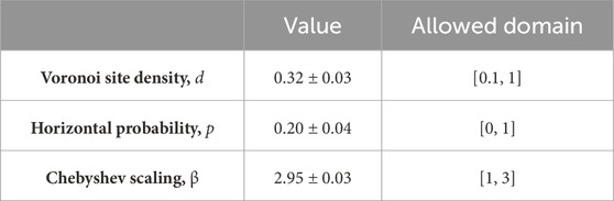
TABLE 1. Obtained ensemble parameter values. The first column shows the average value and the standard deviation measured over the 411 solutions, whose p ≤0.5, collected over all generations and all independent optimization processes, and whose fitness value is in one standard deviation from the fifth peak (red) in Figure 5D. The second column shows the allowed domain of parameters for genetic optimization.

3 Results

Figure 6A shows the spectral entropy curve measured over the 25 ground truth networks (blue curve) and the spectral entropy measured for the synthetic networks generated with the optimized parameters (red curve). A significant alignment between the curves is observed for almost all values of the normalized time τ, thus, over all scales, indicating the overall similarity of the structural connectivity between the network ensembles of the synthetic and ground truth networks. The matched upper bound indicates almost the same average number of nodes between the ensembles of the ground truth networks and the synthetic networks (see also Figure 7A). The alignment observed between the two curves can be interpreted as reflecting the information diffusion across both network structures—empirical and synthetic—through nearly identical normalized transient states. At τ ∼ 10², the two curves show the most deviation.

Figure 6B demonstrates a significant alignment between the Laplacian eigenvalue distribution obtained from the ground truth networks and that from the synthetic networks. Nevertheless, we observe that the red curve exhibits a more sudden drop, while the blue curve reveals a smoother decline on the right side of the x-axis. This discrepancy, together with the red curve’s more pronounced peak before the drop at λ ∼ 6, can be attributed to our method’s reduced ability to capture the degree distribution for k ≥ 4 (also depicted in Figure 7C). Figure 6C shows synthetic networks exhibiting visual similarity to the BFO sample shown in Figure 2. More samples are displayed in Supplementary Figure S1.

FIGURE 6

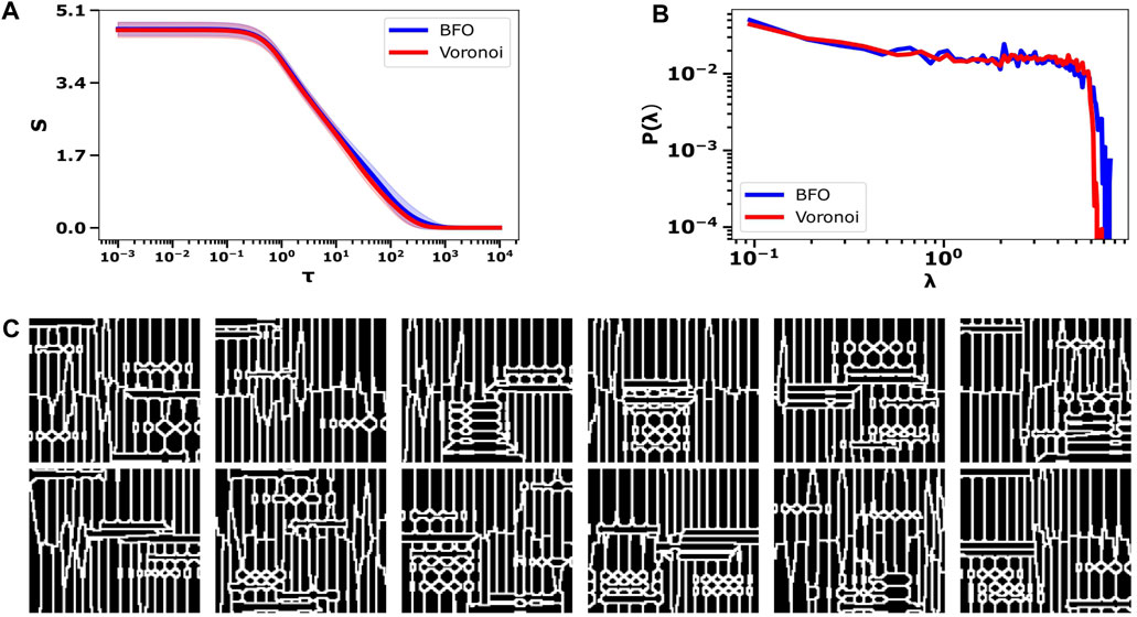
FIGURE 6. (A) Average spectral entropy for both the dataset of 25 annotated networks (blue) and 100 instances of the generated networks (red). The shaded areas indicate the standard deviation. (B) Distribution of Laplacian eigenvalues estimated from the network dataset (blue) and 100 synthetic networks (red). (C) Twelve synthetic exemplary DW networks illustrating a remarkable resemblance to the BFO sample shown in Figure 2.

FIGURE 7

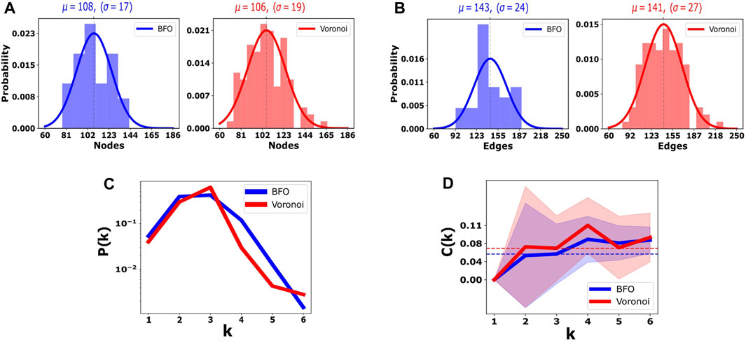
FIGURE 7. Panels (A) and (B) show the node and edge distributions, respectively, for both the ensemble of ground truth networks (blue) and the ensemble of synthetic networks (red). The Gaussian model (continuous line) is fitted to both the distribution of nodes and edges on both the dataset of 25 annotated samples and the generated DW networks (100 samples). The mean parameter, μ, of each Gaussian is indicated by dashed vertical lines, and the corresponding value is illustrated on the top axis together with the standard deviation, σ. Panel (C) shows the probability density function of node degrees, k, for both the ground truth set and the ensemble of generated networks. In (D), the average clustering coefficient C(k) is plotted as a function of the degree, k, for both sets of networks. Shaded area represents the standard deviation.

In panels A and B of Figure 7, the distributions of nodes and edges of both the BFO networks and our model are illustrated. We fitted the Gaussian model to the distributions. The mean, μ, and standard deviation, σ, of each Gaussian are indicated on the top axis. We observed a good match between the Gaussian parameters of the manually annotated dataset (25 samples) and the synthetic dataset generated (100 samples) for both the distributions of nodes and edges. In addition, the spread of the distributions is comparable.

Figure 7C depicts the degree distribution, P(k), for both the manually annotated dataset and the model; as previously mentioned, we observe good matching for smaller degrees and poor matching for larger values of k. In Figure 7D, the clustering coefficient C(k) is plotted as a function of the degree k.

4 Discussion

We introduced a compact and tractable model for creating synthetic instances of DW networks in BFO. While BFO sets the context for this work, we think that our method provides a flexible framework that is potentially applicable to other microstructures as well. Our method involves multiple steps and produces two distinct types of outputs, each with its own relevance: synthetic binary images of DW networks and their graph-based network description. For evaluation, a limited dataset of 25 manually annotated DW networks was created, which, to the best of our knowledge, is the first of its kind. Additionally, our work has led to the development of two tools. The first tool enables the manual annotation of networks from images, assisting efficient labeling of nodes and edges. The second tool tackles the problem of automated network extraction from images and combines pre-existing techniques from the literature.

Our modeling leverages on the centroidal Voronoi tessellation, used to mimic the physical crystal growth on substrates determining the formation of the DW network, and network spectral entropy, which provides a descriptor of the network as a whole across multiple scales, which we used to solve the selection problem of model parameters. Pixel-based instances of DW structures are produced with the centroidal Voronoi tessellation with a combined vertical and horizontal axial-scaled Chebyshev distance. Only three parameters govern the obtained patterns: the linear density of Voronoi sites on the image, d; the axial scale of the Chebyshev distance, β; and the probability of scaling along either the vertical or horizontal axis, p. Even though the Voronoi process is unrelated to the physical growth of polarization domains in the material, the Voronoi regions can be interpreted as analogous to the polarization domains, and the borders between Voronoi regions can be interpreted as analogous to the DWs in the physical sample.

In this work, we are mainly interested in a graph description of the DW network of the BFO as we aim to reproduce the topological properties of BFO DW networks and, in future works, complement it with a dynamical model describing the memristive conductive properties of the DWs, thus merging the current work with our previous work on disordered memristive networks with Ohmic impurities (Cipollini and Schomaker, 2023). Thus, the network of DWs is subsequently automatically extracted from the pixel-based sample, and the parameters of the Voronoi generation process are optimized using a non-gradient genetic algorithm by means of a novel information-theoretic tool for characterizing complex networks, the von Neumann entropy, or spectral entropy. Such a theoretical tool proves to be a good descriptor across all spatiotemporal scales of a heterogeneous network. The formal framework introduced by Domenico and Biamonte (2016) is grounded in statistical physics and leverages on the extension of the concept of a canonical ensemble to graphs. The canonical ensemble comprises the set of all networks with a fixed number of nodes obtained by fixing the expected values of the chosen constraints. In our case, the Voronoi tessellation method does not allow for a fixed number of nodes; thus, the ensemble hypotheses are arbitrarily relaxed in this work, and the spectral entropy is then used to provide a descriptor encoding the structural properties of the network as a whole, rather than using a subset of network properties. The convergence of the algorithm results in progressive lower distances between the spectral entropy estimated for the ground truth ensemble and the Voronoi-based synthetic ensemble, empirically demonstrating that the defined similarity function in Section 2.3 can be interpreted as a proxy of the more rigorous relative entropy introduced by Domenico and Biamonte (2016). The choice of fitting the spectral entropy reflects our focus on the diffusion of information over the network and can be thought of as fitting the transient diffusion modes. After fitting, a good alignment has been observed between multiple network descriptors. The good matching of the spectral entropy curves reflects the ability of the Voronoi tessellation to mimic the growth process of the material as such an alignment would not be a necessary result of any model. In addition, the eigenvalue and the degree distributions computed over the two ensembles show a good match. Nevertheless, a poor alignment is observed for larger eigenvalues (λ ≥ 6) and degree k > 4. A good fit is also evident from the average numbers of nodes and edges. However, two limitations need to be mentioned. The manually annotated dataset is small and unavoidably subject to possible human error. The image-based automated network extraction contains heuristics that may pose biases in the graph construction. Both these conditions can be mitigated in future research. There exist other computational models for the generation of pixel-based DW microstructures that may enhance the similarity to the empirical ones. For instance, the generalization of Laguerre tessellations, the so-called generalized balanced power diagrams (GBPDs), produces non-convex cells and curved faces, which is different from what can be obtained with the standard Voronoi and Laguerre tessellations. However, the utilization of GBPDs may result in increased computational costs. This study provides a new level of analysis of experimental BFO samples, which may help in understanding the physical properties of the substrate, evaluating its usability for neuromorphic computing, and, ultimately, proposing DW deposition patterns which have the desired properties for neuromorphic computing.

Data availability statement

The original contributions presented in the study are included in the article/Supplementary Material; further inquiries can be directed to the corresponding authors.

Author contributions

DC: conceptualization, data curation, software, writing–original draft, writing–review and editing, and methodology. AS: writing–review and editing, software, and data curation. LS: funding acquisition, supervision, writing–review and editing, and conceptualization.

Funding

The author(s) declare that financial support was received for the research, authorship, and/or publication of this article. This work was funded by EUs Horizon 2020, from the MSCA-ITN-2019 Innovative Training Networks program “Materials for Neuromorphic Circuits” (MANIC) under the grant agreement no. 861153, and by the financial support of the CogniGron research center and the Ubbo Emmius Funds (University of Groningen).

Acknowledgments

The authors are grateful to Beatriz Noheda and Jan Rieck for their invaluable assistance in providing them with the cAFM data and for the discussions regarding their concept of applying domain wall networks in nanoelectronics. The authors are grateful to Gilles Bonnet for the useful discussion on stochastic geometry.

Conflict of interest

The authors declare that the research was conducted in the absence of any commercial or financial relationships that could be construed as a potential conflict of interest.

Publisher’s note

All claims expressed in this article are solely those of the authors and do not necessarily represent those of their affiliated organizations, or those of the publisher, the editors, and the reviewers. Any product that may be evaluated in this article, or claim that may be made by its manufacturer, is not guaranteed or endorsed by the publisher.

Supplementary material

The Supplementary Material for this article can be found online at: https://www.frontiersin.org/articles/10.3389/fmats.2024.1323153/full#supplementary-material

References

Anand, O. (2012). Micromechanical modeling of ferroelectric thin films and bulk ceramics in a multi-scale approach. Ph.D. thesis. Stuttgart Germany: Universität Stuttgart. doi:10.18419/OPUS-5081

CrossRef Full Text | Google Scholar

Anderson, W. N., and Morley, T. D. (1985). Eigenvalues of the laplacian of a graph. Linear Multilinear Algebra 18, 141–145. doi:10.1080/03081088508817681

CrossRef Full Text | Google Scholar

Bose, S. K., Mallinson, J. B., Gazoni, R. M., and Brown, S. A. (2017). Stable self-assembled atomic-switch networks for neuromorphic applications. IEEE Trans. Electron Devices 64, 5194–5201. doi:10.1109/TED.2017.2766063

CrossRef Full Text | Google Scholar

Caravelli, F., Milano, G., Ricciardi, C., and Kuncic, Z. (2023). Mean field theory of self-organizing memristive connectomes. Ann. Phys. 535. doi:10.1002/andp.202300090

CrossRef Full Text | Google Scholar

Caravelli, F., Sheldon, F. C., and Traversa, F. L. (2021). Global minimization via classical tunneling assisted by collective force field formation. Sci. Adv. 7, eabh1542. doi:10.1126/sciadv.abh1542

PubMed Abstract | CrossRef Full Text | Google Scholar

Catalan, G., Seidel, J., Ramesh, R., and Scott, J. F. (2012). Domain wall nanoelectronics. Rev. Mod. Phys. 84, 119–156. doi:10.1103/RevModPhys.84.119

CrossRef Full Text | Google Scholar

Chen, D., Tan, X., Shen, B., and Jiang, J. (2023). Erasable domain wall current-dominated resistive switching in BiFeO₃ devices with an oxide-metal interface. ACS Appl. Mater. Interfaces 15, 25041–25048. doi:10.1021/acsami.3c02710

PubMed Abstract | CrossRef Full Text | Google Scholar

Chen, J., Yang, G., and Yang, M. (2019). Computation of compact distributions of discrete elements. Algorithms 12, 41. doi:10.3390/a12020041

CrossRef Full Text | Google Scholar

Chiu, Y.-P., Chen, Y.-T., Huang, B.-C., Shih, M.-C., Yang, J.-C., He, Q., et al. (2011). Atomic-scale evolution of local electronic structure across multiferroic domain walls. Adv. Mater. 23, 1530–1534. doi:10.1002/adma.201004143

PubMed Abstract | CrossRef Full Text | Google Scholar

Christensen, D. V., Dittmann, R., Linares-Barranco, B., Sebastian, A., Gallo, M. L., Redaelli, A., et al. (2022). 2022 roadmap on neuromorphic computing and engineering. Neuromorphic Comput. Eng. 2, 022501. doi:10.1088/2634-4386/ac4a83

CrossRef Full Text | Google Scholar

Cimini, G., Squartini, T., Saracco, F., Garlaschelli, D., Gabrielli, A., and Caldarelli, G. (2019). The statistical physics of real-world networks. Nat. Rev. Phys. 1, 58–71. doi:10.1038/s42254-018-0002-6

CrossRef Full Text | Google Scholar

Cipollini, D., and Schomaker, L. (2023). Conduction and entropy analysis of a mixed memristor-resistor model for neuromorphic networks. Neuromorphic Comput. Eng. 3, 034001. doi:10.1088/2634-4386/acd6b3

CrossRef Full Text | Google Scholar

Dirnberger, M., Kehl, T., and Neumann, A. (2015). NEFI: network extraction from images. Sci. Rep. 5, 15669. doi:10.1038/srep15669

PubMed Abstract | CrossRef Full Text | Google Scholar

Domenico, M. D., and Biamonte, J. (2016). Spectral entropies as information-theoretic tools for complex network comparison. Phys. Rev. X 6, 041062. doi:10.1103/physrevx.6.041062

CrossRef Full Text | Google Scholar

Efros, A. A., and Leung, T. K. (1999). “Texture synthesis by non-parametric sampling,” in Proceedings of the seventh IEEE international conference on computer vision, Kerkyra, Greece, September 1999 (IEEE), 1033–1038.

CrossRef Full Text | Google Scholar

Ellens, W., Spieksma, F., Mieghem, P. V., Jamakovic, A., and Kooij, R. (2011). Effective graph resistance. Linear Algebra its Appl. 435, 2491–2506. doi:10.1016/j.laa.2011.02.024

CrossRef Full Text | Google Scholar

Estrada, E. (2011). The structure of complex networks: theory and applications. USA: Oxford University Press, Inc.

Google Scholar

Farokhipoor, S., and Noheda, B. (2011). Conduction through 71°domain walls in BiFeO₃ thin films. Phys. Rev. Lett. 107, 127601. doi:10.1103/PhysRevLett.107.127601

PubMed Abstract | CrossRef Full Text | Google Scholar

Farokhipoor, S., and Noheda, B. (2012). Local conductivity and the role of vacancies around twin walls of (001)-BiFeO₃ thin films. J. Appl. Phys. 112, 052003. doi:10.1063/1.4746073

CrossRef Full Text | Google Scholar

Feigl, L., Yudin, P., Stolichnov, I., Sluka, T., Shapovalov, K., Mtebwa, M., et al. (2014). Controlled stripes of ultrafine ferroelectric domains. Nat. Commun. 5, 4677. doi:10.1038/ncomms5677

PubMed Abstract | CrossRef Full Text | Google Scholar

Feynman, R. P. (1998). Statistical mechanics: a set of lectures. Boca Raton, Florida: CRC Press. doi:10.1201/9780429493034

CrossRef Full Text | Google Scholar

Gad, A. F. (2021). Pygad: an intuitive genetic algorithm python library. https://arxiv.org/abs/2106.06158.

Google Scholar

Ghavasieh, A., and De Domenico, M. (2023). Generalized network density matrices for analysis of multiscale functional diversity. Phys. Rev. E 107, 044304. doi:10.1103/PhysRevE.107.044304

PubMed Abstract | CrossRef Full Text | Google Scholar

Ghavasieh, A., Nicolini, C., and Domenico, M. D. (2020). Statistical physics of complex information dynamics. Phys. Rev. E 102, 052304. doi:10.1103/physreve.102.052304

PubMed Abstract | CrossRef Full Text | Google Scholar

He, S., Wiering, M., and Schomaker, L. (2015). Junction detection in handwritten documents and its application to writer identification. Pattern Recognit. 48, 4036–4048. doi:10.1016/j.patcog.2015.05.022

CrossRef Full Text | Google Scholar

Ho, C.-W., Ruehli, A., and Brennan, P. (1975). The modified nodal approach to network analysis. IEEE Trans. Circuits Syst. 22, 504–509. doi:10.1109/tcs.1975.1084079

CrossRef Full Text | Google Scholar

Hochstetter, J., Zhu, R., Loeffler, A., Diaz-Alvarez, A., Nakayama, T., and Kuncic, Z. (2021). Avalanches and edge-of-chaos learning in neuromorphic nanowire networks. Nat. Commun. 12, 4008. doi:10.1038/s41467-021-24260-z

PubMed Abstract | CrossRef Full Text | Google Scholar

Indiveri, G., Linares-Barranco, B., Legenstein, R., Deligeorgis, G., and Prodromakis, T. (2013). Integration of nanoscale memristor synapses in neuromorphic computing architectures. Nanotechnology 24, 384010. doi:10.1088/0957-4484/24/38/384010

PubMed Abstract | CrossRef Full Text | Google Scholar

Jia, C.-L., Mi, S.-B., Urban, K., Vrejoiu, I., Alexe, M., and Hesse, D. (2007). Atomic-scale study of electric dipoles near charged and uncharged domain walls in ferroelectric films. Nat. Mater. 7, 57–61. doi:10.1038/nmat2080

PubMed Abstract | CrossRef Full Text | Google Scholar

Kanopoulos, N., Vasanthavada, N., and Baker, R. L. (1988). Design of an image edge detection filter using the sobel operator. IEEE J. solid-state circuits 23, 358–367. doi:10.1109/4.996

CrossRef Full Text | Google Scholar

Kittel, C. (1946). Theory of the structure of ferromagnetic domains in films and small particles. Phys. Rev. 70, 965–971. doi:10.1103/PhysRev.70.965

CrossRef Full Text | Google Scholar

Klein, D. J., and Randić, M. (1993). Resistance distance. J. Math. Chem. 12, 81–95. doi:10.1007/bf01164627

CrossRef Full Text | Google Scholar

Landau, L., and Lifshitz, E. (1992). On the theory of the dispersion of magnetic permeability in ferromagnetic bodies. Amsterdam, Netherlands: Elsevier, 51–65. doi:10.1016/b978-0-08-036364-6.50008-9

CrossRef Full Text | Google Scholar

Liu, Z., Wang, H., Li, M., Tao, L., Paudel, T. R., Yu, H., et al. (2023). In-plane charged domain walls with memristive behaviour in a ferroelectric film. Nature 613, 656–661. doi:10.1038/s41586-022-05503-5

PubMed Abstract | CrossRef Full Text | Google Scholar

Lloyd, S. (1982). Least squares quantization in PCM. IEEE Trans. Inf. Theory 28, 129–137. doi:10.1109/tit.1982.1056489

CrossRef Full Text | Google Scholar

Loeffler, A., Zhu, R., Hochstetter, J., Li, M., Fu, K., Diaz-Alvarez, A., et al. (2020). Topological properties of neuromorphic nanowire networks. Front. Neurosci. 14, 184. doi:10.3389/fnins.2020.00184

PubMed Abstract | CrossRef Full Text | Google Scholar

Maksymovych, P., Seidel, J., Chu, Y. H., Wu, P., Baddorf, A. P., Chen, L.-Q., et al. (2011). Dynamic conductivity of ferroelectric domain walls in BiFeO₃. Nano Lett. 11, 1906–1912. doi:10.1021/nl104363x

PubMed Abstract | CrossRef Full Text | Google Scholar

Mambretti, F., Mirigliano, M., Tentori, E., Pedrani, N., Martini, G., Milani, P., et al. (2022). Dynamical stochastic simulation of complex electrical behavior in neuromorphic networks of metallic nanojunctions. Sci. Rep. 12, 12234. doi:10.1038/s41598-022-15996-9

PubMed Abstract | CrossRef Full Text | Google Scholar

Mannocci, P., Farronato, M., Lepri, N., Cattaneo, L., Glukhov, A., Sun, Z., et al. (2023). In-memory computing with emerging memory devices: status and outlook. Apl. Mach. Learn. 1. doi:10.1063/5.0136403

CrossRef Full Text | Google Scholar

Masuda, N., Porter, M. A., and Lambiotte, R. (2017). Random walks and diffusion on networks. Phys. Rep. 716-717, 1–58. doi:10.1016/j.physrep.2017.07.007

CrossRef Full Text | Google Scholar

Mead, C. (2020). How we created neuromorphic engineering. Nat. Electron. 3, 434–435. doi:10.1038/s41928-020-0448-2

CrossRef Full Text | Google Scholar

Meier, D., Seidel, J., Cano, A., Delaney, K., Kumagai, Y., Mostovoy, M., et al. (2012). Anisotropic conductance at improper ferroelectric domain walls. Nat. Mater. 11, 284–288. doi:10.1038/nmat3249

PubMed Abstract | CrossRef Full Text | Google Scholar

Meier, D., and Selbach, S. M. (2022). Ferroelectric domain walls for nanotechnology. Nat. Rev. Mater. 7, 157–173. doi:10.1038/s41578-021-00375-z

CrossRef Full Text | Google Scholar

Milano, G., Miranda, E., and Ricciardi, C. (2022). Connectome of memristive nanowire networks through graph theory. Neural Netw. 150, 137–148. doi:10.1016/j.neunet.2022.02.022

PubMed Abstract | CrossRef Full Text | Google Scholar

Milano, G., Pedretti, G., Montano, K., Ricci, S., Hashemkhani, S., Boarino, L., et al. (2021). In materia reservoir computing with a fully memristive architecture based on self-organizing nanowire networks. Nat. Mater. 21, 195–202. doi:10.1038/s41563-021-01099-9

PubMed Abstract | CrossRef Full Text | Google Scholar

Mitchell, M. (1998). An introduction to genetic algorithms. Cambridge, Massachusetts: MIT press.

Google Scholar

Montano, K., Milano, G., and Ricciardi, C. (2022). Grid-graph modeling of emergent neuromorphic dynamics and heterosynaptic plasticity in memristive nanonetworks. Neuromorphic Comput. Eng. 2, 014007. doi:10.1088/2634-4386/ac4d86

CrossRef Full Text | Google Scholar

Moreno, Y., and Pacheco, A. F. (2004). Synchronization of kuramoto oscillators in scale-free networks. Europhys. Lett. (EPL) 68, 603–609. doi:10.1209/epl/i2004-10238-x

CrossRef Full Text | Google Scholar

Nesterov, O., Matzen, S., Magen, C., Vlooswijk, A. H. G., Catalan, G., and Noheda, B. (2013). Thickness scaling of ferroelastic domains in PbTiO₃ films on DyScO₃. Appl. Phys. Lett. 103, 142901. doi:10.1063/1.4823536

CrossRef Full Text | Google Scholar

Newman, M. (2010). Networks. Oxford, UK: Oxford University Press. doi:10.1093/acprof:oso/9780199206650.001.0001

CrossRef Full Text | Google Scholar

Nicolini, C., Forcellini, G., Minati, L., and Bifone, A. (2020). Scale-resolved analysis of brain functional connectivity networks with spectral entropy. Neuroimage 211, 116603. doi:10.1016/j.neuroimage.2020.116603

PubMed Abstract | CrossRef Full Text | Google Scholar

Nicolini, C., Vlasov, V., and Bifone, A. (2018). Thermodynamics of network model fitting with spectral entropies. Phys. Rev. E 98, 022322. doi:10.1103/PhysRevE.98.022322

PubMed Abstract | CrossRef Full Text | Google Scholar

Pastor-Satorras, R., and Vespignani, A. (2001). Epidemic spreading in scale-free networks. Phys. Rev. Lett. 86, 3200–3203. doi:10.1103/physrevlett.86.3200

PubMed Abstract | CrossRef Full Text | Google Scholar

Profumo, F., Borghi, F., Falqui, A., and Milani, P. (2023). Potentiation and depression behaviour in a two-terminal memristor based on nanostructured bilayer ZrO_x/au films. J. Phys. D Appl. Phys. 56, 355301. doi:10.1088/1361-6463/acd704

CrossRef Full Text | Google Scholar

Rieck, J. L., Cipollini, D., Salverda, M., Quinteros, C. P., Schomaker, L. R. B., and Noheda, B. (2022). Ferroelastic domain walls in BiFeO₃ as memristive networks. Adv. Intell. Syst. 5, 2200292. doi:10.1002/aisy.202200292

CrossRef Full Text | Google Scholar

Šedivý, O., Brereton, T., Westhoff, D., Polívka, L., Beneš, V., Schmidt, V., et al. (2016). 3d reconstruction of grains in polycrystalline materials using a tessellation model with curved grain boundaries. Philos. Mag. 96, 1926–1949. doi:10.1080/14786435.2016.1183829

CrossRef Full Text | Google Scholar

Seidel, J., Martin, L. W., He, Q., Zhan, Q., Chu, Y.-H., Rother, A., et al. (2009). Conduction at domain walls in oxide multiferroics. Nat. Mater. 8, 229–234. doi:10.1038/nmat2373

PubMed Abstract | CrossRef Full Text | Google Scholar

Strogatz, S. H. (2001). Exploring complex networks. Nature 410, 268–276. doi:10.1038/35065725

PubMed Abstract | CrossRef Full Text | Google Scholar

Suárez, L. E., Richards, B. A., Lajoie, G., and Misic, B. (2021). Learning function from structure in neuromorphic networks. Nat. Mach. Intell. 3, 771–786. doi:10.1038/s42256-021-00376-1

CrossRef Full Text | Google Scholar

Villegas, P., Gabrielli, A., Santucci, F., Caldarelli, G., and Gili, T. (2022). Laplacian paths in complex networks: information core emerges from entropic transitions. Phys. Rev. Res. 4, 033196. doi:10.1103/physrevresearch.4.033196

CrossRef Full Text | Google Scholar

Villegas, P., Gili, T., Caldarelli, G., and Gabrielli, A. (2023). Laplacian renormalization group for heterogeneous networks. Nat. Phys. 19, 445–450. doi:10.1038/s41567-022-01866-8

CrossRef Full Text | Google Scholar

Vlooswijk, A. H. G., Noheda, B., Catalan, G., Janssens, A., Barcones, B., Rijnders, G., et al. (2007). Smallest 90° domains in epitaxial ferroelectric films. Appl. Phys. Lett. 91. doi:10.1063/1.2783274

CrossRef Full Text | Google Scholar