Nonlinear dynamics and stability analysis of locally active Mott memristors using a physics-based compact model

Locally active memristors (LAMs) are a class of emerging nonlinear dynamic circuit elements that hold promise for scalable yet biomimetic neuromorphic circuits. Starting from a physics-based compact model, we performed small-signal linearization analyses and applied Chua’s local activity theory to a one-dimensional, locally active vanadium dioxide Mott memristor based on an insulator-to-metal phase transition. This approach establishes a connection between the dynamical behaviors of a Mott memristor and its physical device parameters, enabling a complete mapping of the locally passive and edge-of-chaos domains in the frequency and current operating parameter space. This mapping could guide materials and device development for neuromorphic circuit applications. We also examined the applicability of local analyses to a second-order relaxation oscillator circuit, which consists of a voltage-biased vanadium dioxide memristor coupled to a parallel reactive capacitor element and a series resistor. Chua’s local activity criteria allows a mapping of this second-order system’s dynamics and stability in the frequency and circuit parameter space, which is essentially a phase diagram for complexity. It shows that the coupling increases both the system’s dimension and its dynamical complexity and creates a locally active and unstable region to host instabilities and persistent oscillations. We show that global nonlinear techniques, including nullclines and phase portraits, provide further insights into instabilities and persistent oscillations near non-hyperbolic fixed points. Specifically, we observe a supercritical Hopf-like bifurcation, where an orbitally stable limit cycle emerges as a new attractor when a stable spiral transitions to an unstable one, with each of the three circuit parameters acting as a bifurcation parameter. The abrupt growth of the limit cycle resembles the Canard explosion phenomenon observed in systems exhibiting relaxation oscillations. Finally, we show that experimental limit cycle oscillations in a vanadium dioxide nano-device relaxation oscillator closely match SPICE simulations based on the compact model.

1 Introduction

In recent years, a surge of interest has been witnessed in exploiting nonlinear dynamical phenomena in emerging devices for novel circuit applications, such as neuromorphic computing. A subject that has been intensively studied is one-port (two-terminal) passive memristors, which exhibit a pinched hysteresis that always passes through the origin in their current–voltage (I–V) loci, thereby possessing a non-volatile memory effect (Strukov et al., 2008; Dittmann and Strachan, 2019). Passive memristors offer a scalable and energy-efficient approach to emulating biological synapses and implementing computationally efficient neuromorphic learning rules (Kim et al., 2015; Wang et al., 2017; Covi et al., 2018; Brivio et al., 2021).

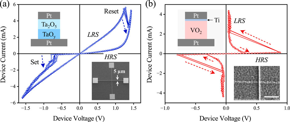
Although a canonical memristor is a passive circuit element, any one-port device that exhibits a pinched hysteresis is considered an extended memristor (Chua, 2014), which includes a class of one-port devices that exhibit non-monotonicity in their experimental quasi-direct current (quasi-DC) I–V curves—a negative differential resistance (NDR). These devices typically exhibit a pronounced I–V hysteresis when driven by a voltage stimulus; however, the hysteresis collapses at a finite voltage. Therefore, they only have a transient (volatile) memory effect. Importantly, these globally passive one-port devices are locally active within the NDR region. Under proper biasing conditions, they can function as one-port amplifiers that increase the power of an alternating-current (AC) signal applied to the same port. It was recently shown that a locally active memristor (LAM) in a distributed form can act as an axon-like signal-amplifying transmission line (Brown et al., 2024). Signal amplification is an essential capability for information processing and communication, a field that has been dominated by transistors. Figure 1 shows the comparison of typical quasi-DC I–V curves measured from a passive memristor and a locally active memristor. Such a measurement varies V or I stimulus slowly and measures time-averaged device responses, which could capture the resistance states before and after a resistance switching event (see arrows) but not the ultrafast switching dynamics that could occur within femtoseconds. Figure 1A shows a bipolar tantalum oxide (${\text{TaO}}_y$-${\text{Ta}}_2{\text{O}}_5$) passive memristor, which switches from a low-resistance state (LRS) to a high-resistance state (HRS) if a sufficiently large positive voltage is applied (Reset) and switches from the HRS back to the LRS if a sufficiently large negative voltage is applied (Set). Both Reset and Set operations are nonvolatile, i.e., resistance changes are retained even after power is turned off. In contrast, Figure 1B shows a unipolar vanadium dioxide (${\text{VO}}_2$) locally active memristor, which abruptly switches from an HRS to an LRS if a sufficiently large voltage is applied, regardless of its polarity. As the voltage is reduced below a smaller threshold level, the device switches from the LRS back to the HRS—these resistance changes are volatile and are lost once the power is turned off. It should be noted that the exemplary characteristics in Figure 1 are by no means exhaustive. Passive memristors can exhibit either bipolar or unipolar non-volatile resistance switching behaviors, which are determined by the intertwined ionic and electronic transport mechanisms within the nanoscale device volume (Waser et al., 2009; Jeong et al., 2012). They may also exhibit a fading memory effect, where the asymptotic behavior is solely determined by the state dynamics, irrespective of the initial condition (Ascoli et al., 2016; Pershin and Slipko, 2019).

Figure 1

Figure 1. Experimental quasi-DC I–V curves for (A) a ${\text{TaO}}_y$-${\text{Ta}}_2{\text{O}}_5$ bilayer passive memristor and (B) a ${\text{VO}}_2$ locally active memristor, constructed and characterized by HRL Laboratories, LLC. Resistance switching events are indicated by dashed arrows. (A) These insets show the layer structure and optical image of the $5\times 5$ $\mathrm{\mu }{\text{m}}^2$ ${\text{TaO}}_y$-${\text{Ta}}_2{\text{O}}_5$ ($y<2$) crossbar device. (B) These insets show the layer structure and scanning electron micrograph of the $50\times 50$ ${\text{nm}}^2$ ${\text{VO}}_2$ nano-crossbar device (scale bar: 500 nm). Memristor crossbars are tested in a four-terminal Kelvin connection (see Yi et al. (2019) for details). The external voltage is swept at $\sim$1 V/s rate in the sequence of 0 $\to$ +$V_{\text{p}}$ $\to$ 0 $\to$ –$V_{\text{n}}$ $\to$ 0 (repeated 10 times). $V_{\text{p}}(V_{\text{n}})=2.5(2)$ V in (A) and $V_{\text{p,n}}=1.45$ V in (B). The metal electrodes contribute a series resistance of 600–800 $\mathrm{\Omega }$.

We now focus on one-port devices that possess the peculiar I–V characteristics shown in Figure 1B. One-port devices with such switching characteristics have been extensively studied and implemented in engineering practice. They have been made out of many materials based on a variety of operating mechanisms. A familiar category is electro-thermal threshold switches such as ovonic threshold switches (OTSs), which show rapid changes in resistance due to nonlinear interactions among local temperature, metastable structural change, and electrical conductivity (Ovshinsky, 1968; Noé et al., 2020). Being a one-port device, LAMs and passive memristors share the same level of ${4\text{F}}^2$ (F: half pitch in lithography) scalability in a crossbar device geometry (Amsinck et al., 2005), resolving the trade-off between scalability and biological fidelity.

LAMs may generally be classified into two types, namely, current-controlled (S-type) and voltage-controlled ($\lambda$-type), where the letters “S” and “$\lambda$” resemble the characteristic shape of NDR in the I–V curve plotted with voltage as the $x$-axis (Ridley, 1963). S-type LAMs are “normally off” devices with an HRS when the power is turned off. $\lambda$-type LAMs such as resonant tunneling diodes are “normally on” devices with an LRS when the power is turned off (Esaki, 1958). Therefore, S-type LAMs are superior to $\lambda$-type LAMs in terms of standby power consumption. Hereafter, we focus our discussion on current-controlled LAMs.

A particularly interesting class of current-controlled LAMs is based on the insulator-to-metal phase transition (IMT) phenomena in strongly correlated materials that arise from a coupling between structural distortions (Peierls transition) and electronic instabilities (Mott transition) (Andrews et al., 2019). They possess several attractive features for circuit applications, such as ultralow (femtojoule) switching energy (Prinz et al., 2020), ultra-fast (tens of femtosecond) switching speed (Jager et al., 2017), and electroforming-free operations (Yi et al., 2018). We term all these IMT-based LAMs “Mott memristors” without discerning the subtle differences in their phase transition mechanisms. Vanadium dioxide (${\text{VO}}_2$) and niobium dioxide (${\text{NbO}}_2$) are two intensively studied Mott memristor materials among many others (Andrews et al., 2019).

For neuromorphic computing applications, circuits of self-excited oscillators and spiking neuron emulators have been built with one or more LAMs that are coupled with reactive elements (capacitors) (Farhat and Eldefrawy, 1993; Moon et al., 2015; Ignatov et al., 2015; Stoliar et al., 2017; Wang et al., 2018). An illustrative example is a scalable spiking neuron, which constitutes two oppositely energized (“polarized” in neuroscience glossary) LAMs to mimic the voltage-gated potassium and sodium cell membrane ion channels. When coupled with parallel membrane capacitors and series load resistors, the composite circuit emulates a single-compartment nerve cell, initiating all-or-nothing action potentials upon a suprathreshold stimulus (Yi et al., 2018; Pickett et al., 2013) or acting as a delayed buffer, which allows bidirectional, distortion-free propagation of action potentials when daisy-chained (Pickett and Williams, 2013; Yi, 2022). Such a circuit topology bears some resemblance to a biologically plausible Hodgkin–Huxley (HH) axon model (Chua et al., 2012) and the early 1960s proposals of “neuristor” axons utilizing non-scalable components such as inductors (Crane, 1960; Crane, 1962; Nagumo et al., 1962). Experimental spiking neurons built with ${\text{VO}}_2$ Mott memristors have shown about two dozen biological neuronal temporal dynamics, including all three classes of neuronal excitability (Yi et al., 2018). Arguably, LAM-based neurons and passive memristor-based synapses form a self-sufficient basis to construct a transistorless neural network (Yi and Cruz-Albrecht, 2019).

Despite numerous experimental demonstrations, predictive modeling and analysis of LAM elements and circuits remain challenging and hinder technology development. These difficulties are, in part, due to the fundamental mathematical challenges associated with nonlinear differential systems. One illustrious example is the second part of Hilbert’s $16^{\text{th}}$ problem that questions whether there exists a finite upper bound for the number of limit cycles of planar polynomial differential systems. It remains unsolved today, even for quadratic polynomials (degree $n=2$) (Ilyashenko, 2002). Qualitative local analyses, on the contrary, are facilitated by small-signal linearization techniques, which allow linear analysis to be applied to a nonlinear system near a hyperbolic fixed point with all eigenvalues of the linearization having non-zero real parts (Perko, 1991). A key theoretical contribution made by Chua is the local activity (LA) theorem, which provides a rigorous mathematical definition of the LA as a necessary prerequisite for the emergence of complexity in nonlinear systems (Chua, 2005). Moreover, Chua provided a set of explicit and computable criteria in the parameter space, which allows for identifying the edge-of-chaos (EOC) region that is both locally active and stable, where most of the complexity phenomena emerge. In recent years, Chua’s LA principle has been applied to clarify several long unsolved fundamental problems about dissipative systems, including Prigogine’s symmetry-breaking instability in homogeneous cellular media (Prigogine and Nicolis, 1967); the emergence of Turing instability (Turing, 1952) and its higher-order analog, Smale’s paradox (Smale, 1976), in reaction-diffusion systems; and Hodgkin–Huxley all-or-nothing excitability of nerve cells (Hodgkin and Huxley, 1952). All these complex phenomena are associated with the EOC domain within a system’s parameter space (Ascoli et al., 2022a; Ascoli et al., 2022b; Ascoli et al., 2022c; Chua, 2022).

Mathematically rigorous yet unphysical toy models of nonlinear dynamical elements were frequently used in the LA analysis procedure (Mannan et al., 2016; Mannan et al., 2017). For engineering practice, such toy models fall short of establishing a connection between circuit- or network-level dynamics and the measurable physical properties of constituent components. A recent review thoroughly elaborated on the importance of applying appropriate device physics into the mathematical memristor framework and defining physically relevant model parameters to control the circuit dynamic behavior (Brown et al., 2022b).

The main objective of this manuscript is to apply relevant theoretical techniques to understand the dynamics and stability of nonlinear circuits that involve locally active Mott memristors and map the conditions for the LA regime within the design parameter space (Messaris et al., 2021; Ascoli et al., 2021). These theoretical techniques include essential local analysis methods such as the small-signal linearization and the LA theorem and global techniques such as the nullclines and phase portraits. For engineering relevance, we base our analyses on an analytical one-dimensional (1D) Mott memristor compact model that is built on the laws of thermodynamics and only contains physically relevant device parameters. The model was developed by Pickett and Williams for ${\text{NbO}}_2$ Mott memristors (Pickett and Williams, 2012). Previously, we have verified that it is also applicable to ${\text{VO}}_2$ Mott memristors after replacing the material properties (Oh et al., 2010; Berglund and Guggenheim, 1969), and our SPICE simulations based on this model faithfully reproduced most of the measured neuronal dynamics in neuron circuits built with ${\text{VO}}_2$ memristors (Yi et al., 2018). In this study, we demonstrate that this physics-based compact model is mathematically tractable for applying local and global analysis techniques, with closed-form expressions for all the important quantities involved in the analyses. It enables a connection between the system dynamics and component physical parameters to guide circuit designs and process development. The algorithmic analysis procedure we present using a ${\text{VO}}_2$ Mott memristor model is general in nature and suitable for analyzing other Mott memristor materials. Qualitatively, the predictions regarding the dynamics and stability in this work are similar to those made by compact models based on different choices of state variables and kinetic functions (Brown et al., 2022b).

We focus on theoretical analyses and only included a cursory comparison between the model simulated and experimental characteristics of a ${\text{VO}}_2$ nano-device relaxation oscillator near the end. More detailed comparisons in the context of ${\text{VO}}_2$ Mott memristor neurons can be found in supplementary materials of Yi et al. (2018). It is understood that the compact model presented in this study has some simplifications and limitations. It is a nontrivial task to construct a computationally efficient compact model for locally active memristors with an appropriate balance between the dynamical fidelity and the computational complexity of solving the model equations. This is especially important for digital computer simulations of a scaled network that contains many instances of memristor elements, which could be costly in time and energy consumption.

The remainder of this paper is organized as follows: The first three sections (Sections 2–4) provide the analyses of an isolated 1D Mott memristor. In Section 2, we introduce the physics-based compact model and analyze the stability of an isolated 1D Mott memristor by examining its power-off plot (POP) and dynamic route map under constant input currents or voltages. This exercise confirms that the metallic state of a Mott memristor is unstable without power and is asymptotically stable with a finite input current. It also reveals that varying the voltage as the bifurcation parameter leads to a supercritical saddle-node bifurcation. In Section 3, we solve its locus of steady states (fixed points) in the three-dimensional (3D) state space and their two-dimensional (2D) projections. Note that we use both fixed point and steady state for the same concept in an interchangeable manner but avoid the term equilibrium unless the input is 0. See Subsection 2.2 for an elaboration on this topic.

In Section 4, we apply local analysis techniques on an isolated Mott memristor, including linearization and small-signal analysis, pole–zero diagram, Chua’s LA theorem, and frequency response. Its complex domain ($s$-domain) equivalent circuit derived by the Laplace transform contains three virtual elements—a negative nonlinear capacitor in parallel with a negative nonlinear resistor, both in series with a positive nonlinear resistor. The negative $s$-domain capacitance gives rise to an apparent inductive response, similar to the memristive models of potassium and sodium ion channels (Chua et al., 2012). We found that an isolated Mott memristor near a fixed point dwells either in the locally passive (LP) or the EOC region. The EOC region coincides with the NDR region in its steady state or DC I–V locus. Brown et al. (2022b) explained that for an extended electro-thermal memristor, the coincidence between NDR and EOC or LA regions is not guaranteed. Therefore, NDR shall not be used as a sole signature for EOC. In our case, the crossover between the LP and EOC regions also manifests itself in the small-signal frequency response, which shows a sign reversal in the real part of the impedance (complexity) function Re$Z(s;Q)$, as predicted by the fourth LA criterion. In the frequency domain, an isolated Mott memristor is equivalent to a positive inductor in series with a resistor that is positive in the LP region and negative in the EOC domain. We derived the parametric Nyquist plot of the LP $\leftrightarrow$ EOC crossover at a single current level and then extended it to a 2D color-scale map of Re$Z(s;Q)$ to visualize the LP and EOC regions in the parameter space spanned by frequency and current, which is effectively a phase diagram for complexity. We also examined the scaling trend of the EOC region versus the device size, which shows that the ${\text{VO}}_2$ conduction channel radius is the relevant dimension for device miniaturization to enhance the EOC frequency regime.

Although an EOC region exists in an isolated 1D Mott memristor, the topological constraint limits the dynamics it can possess, making it impossible to exhibit persistent oscillations. In Sections 5–6, we remove the topological constraint for an isolated 1D Mott memristor by coupling it with one or more reactive elements, increasing the system’s dimensionality and dynamical complexity. For simplicity, we choose a DC voltage $(V_{\text{dc}})$-biased Pearson–Anson relaxation oscillator, formed using a Mott memristor coupled with a parallel capacitor $C_{\text{p}}$ and a series resistor $R_{\text{s}}$, as an example of a 2D nonlinear system for our analysis (Pearson and Anson, 1921). The same analysis procedure can be applied to higher-dimensional systems, such as spiking neuron circuits consisting of two or more Mott memristors coupled with passive and reactive elements.

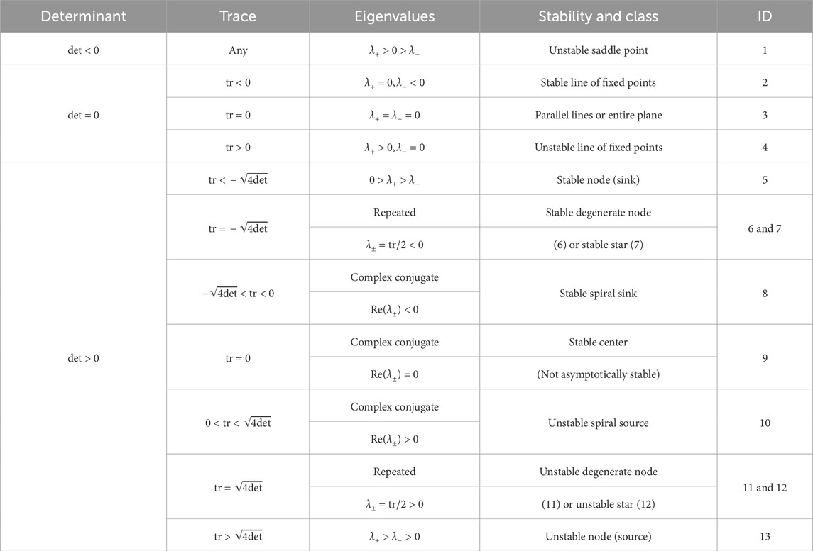
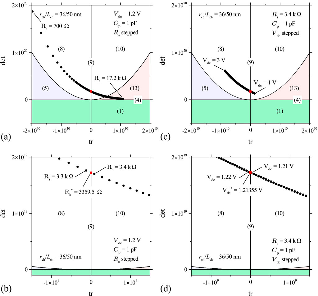
In Section 5 we first apply Chua’s LA criteria and local linearization techniques to this example system, including the element combination approach, the Jacobian matrix method, and the trace-determinant plane classification to study the stability and qualitative behaviors of its hyperbolic fixed points. The element combination approach considers a Mott memristor in parallel with a capacitor to be a composite second-order nonlinear element. The small-signal transfer function of the element-combined system has a pair of complex conjugate or real poles. We derived the Nyquist plot and a 2D phase diagram of the system’s poles. The pole phase diagram, combined with Chua’s LA criteria, allows a visualization of the LP, EOC and locally active and unstable (LA\EOC) regions in the circuit parameter space. These results are corroborated by the trace-determinant plane analysis of the Jacobian linearized 2D system, which reveals a stability-change bifurcation as the parametric (trace and determinant) locus crosses the zero-trace axis as one of the three circuit parameters is varied ($R_{\text{s}}$, $C_{\text{p}}$, and $V_{\text{dc}}$). However, analyzing the stability behavior of a non-hyperbolic center requires additional theoretical tools since the Hartman–Grobman theorem is not applicable due to the loss of hyperbolicity (Hartman, 1960; Grobman, 1959).

Finally, in Section 6 we apply several global methods, such as the nullclines and numerical phase portrait analyses to understand qualitative behaviors of the non-hyperbolic centers in this example 2D nonlinear system. We found that each of the three circuit parameters ($R_{\text{s}}$, $C_{\text{p}}$, and $V_{\text{dc}}$) acts as a bifurcation parameter that switches the stability of a fixed point as the parametric (trace and determinant) locus crosses a center. We verified that there exists a supercritical 2D Hopf-like bifurcation, i.e., the creation of a stable limit cycle encircling an unstable spiral as the fixed point switches its stability from stable to unstable. We also noticed that the limit cycle emerges abruptly over an extremely narrow bifurcation parameter interval, a phenomenon known as “canard explosion” in relaxation oscillations within chemical and biological systems (Krupa and Szmolyan, 2001; Rotstein et al., 2012). This is a prominent distinction from the classical Hopf bifurcation, which predicts a gradual growth proportional to the square root of the bifurcation parameter. Each bifurcation parameter has different bifurcation growth characteristics. We conclude the section with a comparison between the experimental limit cycle characteristics of a ${\text{VO}}_2$ relaxation oscillator and SPICE simulations based on the Mott memristor model, showing excellent agreements between them.

We conclude the manuscript with brief remarks on the application implications of locally active memristors and scalable neuromorphic dynamic neurons with a high degree of complexity.

2 One-dimensional locally active Mott memristor

2.1 Physics-based analytical compact model

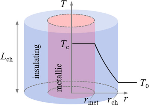
The physics-based compact model for a 1D (one state variable) locally active Mott memristor is biphasic in nature (Pickett and Williams, 2012). It assumes that once an IMT is triggered by Joule self-heating beyond a threshold level, metallic and insulating phases coexist in a constant volume conduction channel defined by the top and bottom electrodes. For mathematical simplification, the conduction channel has an axial symmetry with a constant radius $r_{\text{ch}}$ along its length. An experimental crossbar device may have a square or rectangular cross section defined by its top and bottom electrodes. The insulating phase has significantly lower thermal and electrical conductivity than the metallic phase. Therefore, the core region turns metallic first, and its radius $r_{\text{met}}$ increases as Joule heating increases. In analogy to the case of an ice–water mixture, the maximum temperature within the metallic core is capped to the transition temperature $T_{\text{c}}$ until the whole conduction channel turns metallic. The minimum temperature at the outer edge of the insulator shell is fixed at the ambient temperature $T_0$. The temperature rise required for IMT to occur is defined as $\mathrm{\Delta }T=T_{\text{c}}-T_0$. With these assumptions, a radial temperature profile bounded between $T_0$ and $T_{\text{c}}$ is established across the insulating shell surrounding the metallic core. The schematic representation of this biphasic thermal model is shown in Figure 2.

Figure 2

Figure 2. Schematic representation of the biphasic thermal model for a Mott memristor that undergoes an insulator-to-metal transition, illustrating a cylindrical conduction channel with a metallic-phase core surrounded by an insulating-phase shell. The model assumes that the metallic core is fixed at the transition temperature $T_{\text{c}}$, and the outer edge of the conduction channel is fixed at the ambient temperature $T_0$. The black solid line shows a calculated radial temperature profile. The top and bottom electrodes are not shown for clarity.

The state variable $x\triangleq r_{\text{met}}/r_{\text{ch}}$ is modeled as the dimensionless volumetric fraction of the metallic phase in the conduction channel and is bounded between 0 and 1. The model derives that the temperature at a specific radius $T(r)$ is a nonlinear function of $x$ of the form $T(r)=T_0+\mathrm{\Delta }T\ln (\frac{r}{r_{\text{ch}}})/\ln (x)$, where $r_{\text{met}}\le r\le r_{\text{ch}}$.

Another assumption the model makes for mathematical simplification is to ignore the axial heat exchanges with the electrodes and the associated temperature gradients near the top and bottom interfaces. Moreover, the thermal and electrical conductivity of the insulating shell are approximated as constants, regardless of the radial temperature gradient across it. This approximation holds true if neither of them varies significantly as temperature increases from $T_0$ to $T_{\text{c}}$. This is probably the case for ${\text{VO}}_2$ with a small $\mathrm{\Delta }T$ ($T_{\text{c}}\approx 340$ K and $\mathrm{\Delta }T\approx 43$ K) (Berglund and Guggenheim, 1969) but becomes questionable for ${\text{NbO}}_2$ with a very large $\mathrm{\Delta }T$ ($T_{\text{c}}\approx 1080$ K and $\mathrm{\Delta }T\approx 784$ K) (Janninck and Whitmore, 1966).

The compact model consists of two coupled equations that satisfy the definition of a 1D extended memristor (Chua, 2014): a state-dependent instantaneous relationship between voltage and current in the form of Ohm’s law (state-dependent Ohm’s law) and a first-order ordinary differential equation (ODE) that determines the dynamics of the single state variable $x$ (state equation). The kinetic function that accounts for the state dynamics is a function of both the state variable $x$ and the input variable (voltage $v$ or current $i$). A Mott memristor, therefore, is a dynamical system—a system whose state at a future time depends deterministically on its present sate and a physical law that governs its evolution over time.

Since Joule self-heating depends on the passage of current, a Mott memristor is a current-controlled memristor, and current $i$ instead of voltage $v$ is the appropriate input variable. The model equations take the following form:

$v\left(x,i\right)=R_{\text{ch}}\left(x\right)i,(1)$

$\frac{dx}{dt}\triangleq f_x\left(x,i\right)=\frac{i^2{R}_{\text{ch}}\left(x\right)-{\mathrm{\Gamma }}_{\text{th}}\left(x\right)\mathrm{\Delta }T}{H^{\prime }\left(x\right)}.(2)$

The single state variable $x\in (\mathrm{0,1})$ is a dimensionless quantity within the bounded open interval between 0 and 1. $f_x(x,i)$ is the kinetic function of the state variable $x$. The derivation of $f_x(x,i)$ is nontrivial and is the main task of building the compact model. For Mott memristors and, more generally, electro-thermal memristors, $f_x(x,i)$ is derived from the first law of thermodynamics, which states that the change in the total enthalpy of a system $\mathrm{\Delta }H$ equals the net heat flow $q_p$ into it at constant pressure: $\mathrm{\Delta }H=q_p$. Therefore, their time derivatives are also equal: $\frac{d\mathrm{\Delta }H}{dt}=\frac{d{q}_p}{dt}$. This basic law forms the theoretical basis to interpret electro-thermal memristors, wherein the local temperature change plays a key role. It is worth pointing out that since there is no explicit dependence on time $t$ in $f_x(x,i)$, this is an autonomous system.

To simplify the expression of $f_x(x,i)$, three nonlinear auxiliary functions are defined, namely, the state-dependent memristance function $R_{\text{ch}}(x)$ (Equation 3), the state-dependent thermal conductance function ${\mathrm{\Gamma }}_{\text{th}}(x)$ (Equation 4), and $H^{\prime }(x)\triangleq \frac{d\mathrm{\Delta }H}{dx}$ (Equation 5), which is defined as the derivative of the total enthalpy change $\mathrm{\Delta }H$ with regard to the state variable $x$.

$R_{\text{ch}}\left(x\right)=\frac{1}{A\left(1+B{x}^2\right)},(3)$

${\mathrm{\Gamma }}_{\text{th}}\left(x\right)\mathrm{\Delta }T=-\frac{C}{\ln x},(4)$

$H^{\prime }\left(x\right)\triangleq \frac{d\mathrm{\Delta }H}{dx}=D\left(\frac{1-x^2+2x^2\ln x}{2x{\left(\ln x\right)}^2}+Ex\right),(5)$

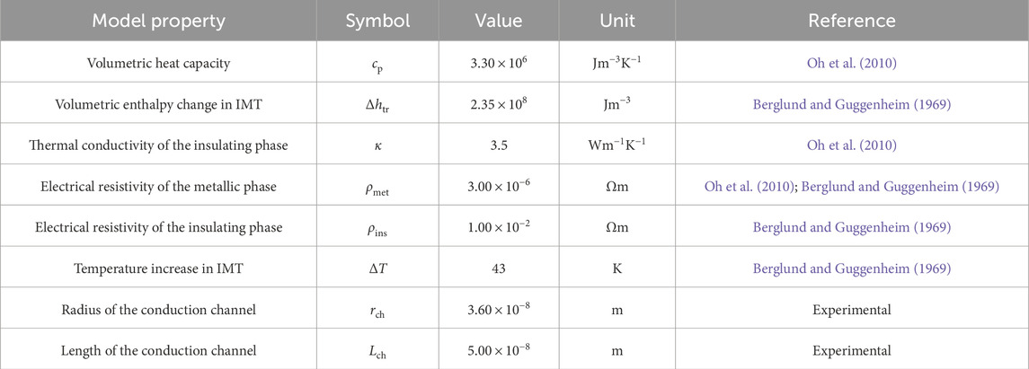
where $A=\frac{\pi r_{\text{ch}}^2}{{\rho }_{\text{ins}}{L}_{\text{ch}}}$, $B=\frac{{\rho }_{\text{ins}}}{{\rho }_{\text{met}}}-1$, $C=2\pi L_{\text{ch}}\kappa \mathrm{\Delta }T$, $D=\pi L_{\text{ch}}{r}_{\text{ch}}^2{c}_{\text{p}}\mathrm{\Delta }T$, and $E=\frac{2\mathrm{\Delta }{h}_{\text{tr}}}{c_{\text{p}}\mathrm{\Delta }T}$ are constant coefficients whose values are determined by physical model parameters, including material properties and device geometry. Table 1 lists the values of these physical model parameters for the case of ${\text{VO}}_2$ material. The radius and length of the memristor conduction channel are device-dependent parameters and can be determined experimentally by the device geometry. The remaining model parameters listed in Table 1 are electronic, thermal, and phase transition properties of ${\text{VO}}_2$ material reported in the literature (Oh et al., 2010; Berglund and Guggenheim, 1969). These material property-dependent parameters can be optimized using a calibration procedure with well-devised characterization of ${\text{VO}}_2$ devices and least-square data fitting (Brown et al., 2022a), but this is beyond the scope of this work.

Table 1

Table 1. Material properties and device parameters of a ${\text{VO}}_2$ Mott memristor model.

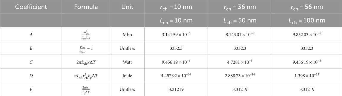
Table 2 lists the values of model coefficients $A$, $B$, $C$, $D$, and $E$ for three arbitrarily chosen ${\text{VO}}_2$ device sizes, including the radius $r_{\text{ch}}$ and length $L_{\text{ch}}$ of the conduction channel. Coefficients $B$ and $E$ are dimensionless and device size-independent. Without loss of generality, these three device sizes are used throughout this manuscript to illustrate the scaling trend of a calculated quantity as the device size varies. If not mentioned explicitly, hereafter, the modeled ${\text{VO}}_2$ device is the medium-sized one in Table 2 with $r_{\text{ch}}=36$ nm and $L_{\text{ch}}=50$ nm, and is referred to as the midsize ${\text{VO}}_2$ Mott memristor or midsize ${\text{VO}}_2$ device.

Table 2

Table 2. Values of model coefficients for three ${\text{VO}}_2$ device sizes.

A more general approach to the physical modeling of an electro-thermal memristor considers the internal temperature the sole state variable (Brown et al., 2022b). The kinetic function is derived from Newton’s law of cooling, which establishes a connection between the net heating power and a time-varying device’s internal temperature through a temperature-dependent thermal capacitance. There is clearly a benefit of adopting a universal state variable and a generalized formula of the kinetic function, albeit the temperature dependence of thermal capacitance is unknown and requires a model fitting with experimental characterization, such as the temperature dependence of self-excited oscillation frequency in a memristor-based relaxation oscillator (Brown et al., 2022a). It is interesting that both approaches can yield the same qualitative predictions regarding the system dynamics, despite differences in model assumptions, state variables, and kinetic functions.

2.2 Stability analyses

We start the stability analyses by focusing on an isolated or uncoupled Mott memristor. The first step is to examine the stability of solutions for Equation 2 by considering the input current to be a parameter with a zero or nonzero constant value and plotting the kinetic function $f_x(x,i)$ as a function of the state variable $x$. If a solution $f_x(x,i)=0$ exists at a point $x_Q$, it is called a fixed point (Shashkin, 1991). This is because the state variable $x(t)$ with an initial condition $x(0)=x_Q$ remains unchanged at any future time, i.e., $x(t)=x_Q$ for $t>0$. The literature from different disciplines has adopted a variety of terminologies for the same concept, including the stationary point, invariant point, equilibrium point, critical point, singular point, and steady-state point. These terms are generally interchangeable but may cause confusion if not carefully chosen. In particular, the use of the equilibrium point may cause misinterpretation by physical scientists for reasons we will elaborate below.

A system at equilibrium remains stable over time and does not require a net flow of energy or work to maintain that condition. A steady state also has stable internal conditions that remain unchanged over time. However, it requires a continuous energy input or work from the external environment to remain in a constant state. A memristor with stable internal states while a finite current flows through it is in a non-equilibrium steady state rather than equilibrium since there is a net heat transfer $q_p$ into the memristor. In this manuscript, we mainly use the term fixed point because of its prevalence in mathematics. Steady state will also be used as a descriptive term when it facilitates interpretation. For example, steady-state resistance is a preferred term over fixed-point resistance.

For a current-controlled memristor, current is the appropriate input variable for stability analysis. However, one can still consider voltage $v$ to be an input and run the same type of analysis. Interestingly, doing so would result in a bifurcation—a qualitative change in the solution of a nonlinear system incurred by a small change in a parameter, such as the creation or annihilation of fixed points or a change in their stability.

2.2.1 Power-off plot

The question of whether a memristor is non-volatile can be answered by examining the power-off plot (Chua, 2015). For a current-controlled memristor, its POP is the locus of the kinetic function $f_x(x,i)$ as a function of the state variable $x$ at zero input current, i.e., the locus of $f_x(x,0)$ vs $x$ (Equation 6).

By setting the input current to 0 in Equation 2, we obtain

$f_x\left(x,0\right)=\frac{-{\mathrm{\Gamma }}_{\text{th}}\left(x\right)\mathrm{\Delta }T}{H^{\prime }\left(x\right)}=\frac{2Cx\ln x}{D\left[1-x^2+2x^2\ln x+2E{\left(x\ln x\right)}^2\right]}.(6)$

If $f_x(x,0)$ has an intersection with the $x$-axis, then the intersection is an equilibrium point $x_Q$. The memristor state $x(t)$ with an initial state $x(0)=x_Q$ remains unchanged at any future time, i.e., $x(t)=x_Q$ for any $t>0$.

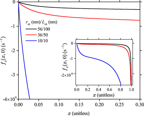
Figure 3 shows that for a Mott memristor at zero input current, $f_x(x,0)$ remains negative for any state variable $x\in (\mathrm{0,1})$. It is plausible since if there were a finite fraction of the conduction channel in the metallic phase at the beginning, it is unstable without the presence of Joule heating and will always vanish over time. The memory effect in a Mott memristor is, therefore, transient or volatile in nature and will be lost, given sufficient time after the removal of electrical power. Figure 3 inset shows that the negative rate of change in $x$ increases dramatically as $x$ approaches 1.0 asymptotically. The calculations are performed using ${\text{VO}}_2$ model parameters, but this conclusion is generally applicable to other Mott memristor materials.

Figure 3

Figure 3. Analytically calculated power-off plots $f_x(x,0)$ vs $x$ for three different-sized ${\text{VO}}_2$ Mott memristors (as labeled) in the small $x$ region $(0<x<0.3)$. Inset shows the same power-off plots for a much wider range of $0<x<1$.

2.2.2 Dynamic route map at constant input current

If input current is fixed at a finite constant level $i_0\ne 0$, one can plot the dynamic route (DR)—the locus of the kinetic function $f_x(x,i_0)$ as a function of the state variable $x$ at a constant input current $i_0$ (Chua, 1969). A set of dynamic routes parameterized by input current (or voltage for a voltage-controlled memristor) is called a dynamic route map (DRM) (Chua, 2018). Rewriting $f_x(x,i)$ in Equation 2 by replacing the auxiliary functions $R_{\text{ch}}(x)$, ${\mathrm{\Gamma }}_{\text{th}}(x)$, and $H^{\prime }(x)$ with their explicit expressions, we obtain

$f_x\left(x,i_0\right)=\frac{\frac{2x{\left(\ln x\right)}^2}{A\left(1+B{x}^2\right)}{i}_0^2+2Cx\ln x}{D\left[1-x^2+2x^2\ln x+2E{\left(x\ln x\right)}^2\right]}.(7)$

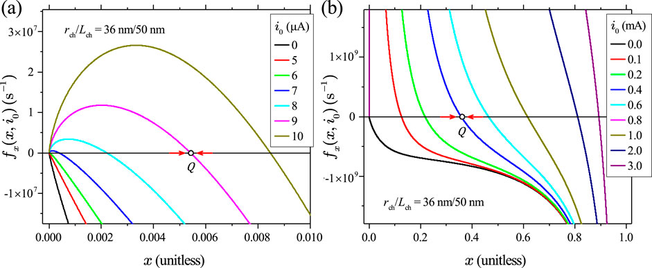
As shown in Figure 4A, even a tiny input current of a few $\mathrm{\mu }$A creates a positive slope for the DR locus of the midsize ${\text{VO}}_2$ device, flipping the fourth-quadrant POP locus up into the first quadrant once a finite current is supplied. The slope of the DR then levels off and becomes negative again as $x$ further increases. Consequently, a constant-current DR locus always intersects the $x$-axis at a single fixed point $x_Q$. This is confirmed by Figure 4B which shows the DRM loci over a much wider current range from 0 to 3 mA.

Figure 4

Figure 4. Analytically calculated dynamic route map of $f_x(x,i_0)$ at constant input current levels for the midsize ${\text{VO}}_2$ Mott memristor, plotted with (A) a narrow range of $i_0$ ranging from 0 to 10 $\mathrm{\mu }$A and (B) a broad range of $i_0$ ranging from 0 to 3 mA. The open circle in (A) and (B) highlights a fixed point $Q$, where the $f_x(x,i_0)$ locus intersects the $x$-axis. Arrowheads show the direction of movement for a solution $x(t)$ starting from an initial state located close to $Q$.

The theory of nonlinear dynamics indicates that the fixed point $x_Q$ is asymptotically stable because the solution $x(t)$ starting from any initial state $x(0)\ne x_Q$ approaches the fixed point $x_Q$ as $t\to \infty$. For $x<x_Q$, $dx/dt>0$. For $x>x_Q$, $dx/dt<0$. The arrowhead pointing to the right indicates that the solution $x(t)$ starting from any initial state $x(0)\ne x_Q$ on the DR above the $x$-axis must move to the right of $x(0)$ because $dx/dt>0$ for $t>0$, as long as $x(t)$ lies above the $x$-axis. Conversely, the arrowhead pointing to the left indicates that the solution $x(t)$ starting from any initial state $x(0)\ne x_Q$ below the $x$-axis on the DR must move to the left of $x(0)$ because $dx/dt<0$ for $t>0$, as long as $x(t)$ lies below the $x$-axis.

2.2.3 Dynamic route map at constant input voltage: saddle-node bifurcation

Although a Mott memristor is a current-controlled device, it is interesting to examine the state dynamics for the case where a constant finite input voltage is applied. Replacing current $i$ by voltage $v$ in Equation 2, the kinetic function can be rewritten as a function of $x$ and $v$. At a constant input voltage $v_0$, it takes the following form:

$\begin{array}{ll}\hfill f_x\left(x,v_0\right)& =\frac{1}{H^{\prime }\left(x\right)}\left(\frac{v_0^2}{R_{\text{ch}}\left(x\right)}-{\mathrm{\Gamma }}_{\text{th}}\left(x\right)\mathrm{\Delta }T\right)\hfill \\ \hfill & =\frac{2Ax{\left(\ln x\right)}^2\left(1+B{x}^2\right)v_0^2+2Cx\ln x}{D\left[1-x^2+2x^2\ln x+2E{\left(x\ln x\right)}^2\right]}.\hfill \end{array}(8)$

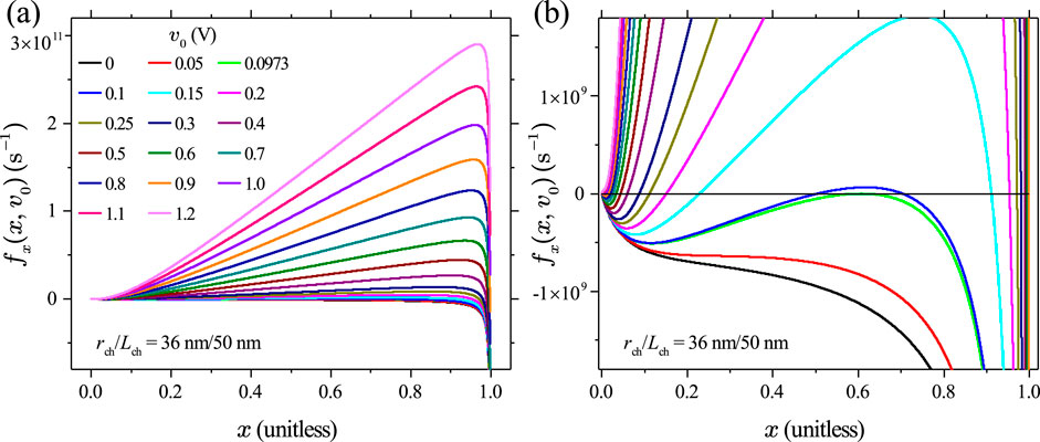
Figure 5A shows the DRM loci of $f_x(x,v_0)$ in Equation 8 vs $x$ at constant $v_0$ levels, ranging from 0 to 1.2 V in 0.1 Vs, interval for the midsize ${\text{VO}}_2$ device. Figure 5B is a zoomed view, which reveals three behaviorally distinctive regions determined by the amplitude of $v_0$. At a very small $v_0<0.0973$ V, the DR locus stays in the fourth quadrant and does not intersect with the $x$-axis. In other words, $f_x(x,v_0)<0$ is satisfied at any $x\in (\mathrm{0,1})$. It indicates that at such small input voltages, even if the initial condition is a metallic phase, a Mott memristor always returns to the insulating state after a finite time. Physically speaking, the Joule heating level at such small voltages is too small to sustain a metallic filament at the IMT critical temperature against the heat loss. At $v_0=0.0973$ V, the DR locus becomes tangent to the $x$-axis with only one intersection point close to $x_0=0.606$. At a $v_0>0.0973$ V, the DR locus “swings” from the fourth quadrant to the first quadrant, and then, it swings back to the fourth quadrant, intersecting the $x$-axis at two distinctive points to the left and right of $x_0$.

Figure 5

Figure 5. (A) Dynamic route map of $f_x(x,v_0)$ at constant input voltages in the range of 0–1.2 V, calculated for the midsize ${\text{VO}}_2$ Mott memristor. (B) Zoomed-in portion of (A) shows that at $v_0>0.0973$ V, the DR locus intersects the $x$-axis at two distinctive locations. At $v_0=0.0973$ V, the DR locus becomes tangent to the $x$-axis with only one intersection point. At $v_0<0.0973$ V, the DR locus stays in the fourth quadrant and does not intersect the $x$-axis.

For a 1D nonlinear ODE system, a saddle-node (tangent) bifurcation is the generic bifurcation in which the number of fixed points changes as a parameter varies. If additional conditions are met, a transcritical or pitchfork bifurcation may occur. A simple example of a saddle-node bifurcation is $dx/dt=\mu \pm x^2$, where $\mu$ is the bifurcation parameter and the sign determines whether it is supercritical $(\mu -x^2)$ or subcritical $(\mu +x^2)$. For the supercritical case, as $\mu$ increases through ${\mu }_0=0$ (the bifurcation value), the number of fixed points changes from 0 to 1 and then to 2. If $\mu <{\mu }_0$, $dx/dt$ is always negative and no fixed point exists. At $\mu ={\mu }_0$, there is one non-hyperbolic, semi-stable fixed point $(x=0)$. At $\mu >{\mu }_0$, a pair of stable $(x=\sqrt{\mu })$ and unstable $(x=-\sqrt{\mu })$ hyperbolic fixed points are created.

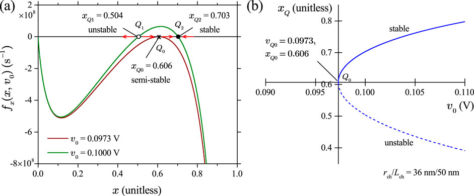
Figure 6 illustrates that if a ${\text{VO}}_2$ Mott memristor is biased by a constant voltage $v_0$, a small change in $v_0$, acting as the bifurcation parameter, results in a supercritical saddle-node bifurcation. For the midsize ${\text{VO}}_2$ device, the bifurcation value for $v_0$ is approximately 0.0973 V. Figure 6A shows the re-plots of the two DRM loci in Figure 5 at $v_0$ levels of 0.0973 V and 0.1 V. At $v_0=0.0973$ V, there is a single semi-stable fixed point $Q_0$ $(\times )$. Increasing the input voltage by a small amount to $v_0=0.1$ V results in a qualitative change in the solution structure and creates a pair of fixed points—the left one $Q_1$ $(◦)$ is unstable and the right one $Q_2$ $(•)$ is stable. The stability of a fixed point is told by the arrowheads, indicating the direction of move for a solution $x(t)$ starting from an initial state located close to it. Figure 6B shows the bifurcation diagram of the 1D saddle-node bifurcation with the input voltage as the bifurcation parameter. Solid and dashed lines show the stable and unstable solutions of fixed points $x_Q$, respectively.

Figure 6

Figure 6. (A) Dynamic routes of $f_x(x,v_0)$ at constant input voltages of 0.0973 V and 0.1 V, calculated for the midsize ${\text{VO}}_2$ Mott memristor. At $v_0=0.0973$ V, the single intersection point $Q_0$ $(\times )$ with the $x$-axis is a semi-stable fixed point. At $v_0=0.1$ V, the left intersection point $Q_1$ $(◦)$ with the $x$-axis is an unstable fixed point, and the right intersection point $Q_2$ $(•)$ with the $x$-axis is a stable fixed point. Arrowheads show the direction of movement for a solution $x(t)$ starting from an initial state located close to a fixed point. (B) Bifurcation diagram of the same device, showing a 1D supercritical saddle-node bifurcation with $v_0$ as the bifurcation parameter. The solid (dashed) line shows the stable (unstable) solutions of fixed points $x_Q$.

3 Loci of steady states

In the present approach, the internal temperature is embedded in the biphasic model and is not considered a state variable. The set of all fixed points $(x_Q,i_Q,v_Q)$ in the 3D $(x,i,v)$ state space that satisfy the instantaneous relationship $v_Q=R_{\text{ch}}(x_Q)i_Q$ and $(dx/dt){|}_Q=0$ is defined as the steady-state or DC locus of a Mott memristor. Solving the steady-state locus of an isolated Mott memristor is among the first steps for the local linearization analysis. Henceforth, both the $(x_Q,i_Q,v_Q)$ locus and its 2D projections are called the steady-state loci without discerning the dimensional difference.

To obtain the steady-state $(x_Q,i_Q,v_Q)$ locus, one can first define a sequence of $i_Q\in \mathbb{R}$ and then find the solutions of the state variable $x=x_Q(i_Q)$ numerically. This is achieved by setting the numerator in Equation 7 to be 0, which provides an equation $CA(1+B{x}_Q^2)=-i_Q^2\ln x_Q$ that can be solved numerically. After solving $x_Q(i_Q)$, voltage $v_Q$ can be calculated using the Ohm’s law relationship $v_Q(i_Q)=R_{\text{ch}}(x_Q(i_Q))i_Q$.

However, there is a much easier way to obtain the steady-state $(x_Q,i_Q,v_Q)$ locus. Instead of numerically solving the value of $x_Q$ from a given $i_Q$, one can first define a sequence of $x_Q\in (\mathrm{0,1})$ and then calculate $i_Q(x_Q)$ analytically using the following formula:

$i_Q\left(x_Q\right)=\sqrt{\frac{-CA\left(1+B{x}_Q^2\right)}{\ln x_Q}}.(9)$

Voltage $v_Q$ is then calculated using the Ohm’s law $v_Q(x_Q)=R_{\text{ch}}(x_Q)i_Q(x_Q)$. The sequence of $x_Q$ can be chosen to be evenly spaced on a linear or logarithmic scale, depending on how fast these functions vary with $x_Q$. We verified that steady states calculated by both methods are consistent with each other. The analytical method is used for discussions hereafter.

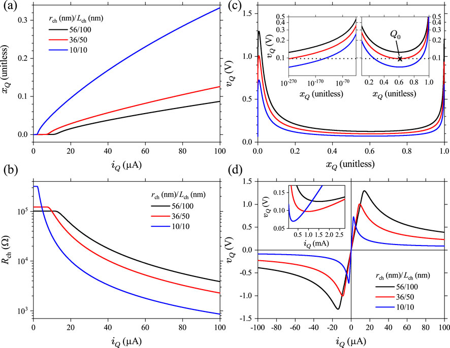
Figure 7A shows the steady-state loci of $(x_Q,i_Q)$ calculated using Equation 9 for three different ${\text{VO}}_2$ device sizes, plotted as $x_Q(i_Q)$, since Mott memristors are current-controlled devices. At small currents, the fraction of the metallic phase $x_Q$ remains negligibly small. $x_Q$ starts to increase with current in a sublinear fashion once $i_Q$ exceeds a size-dependent threshold level. The current threshold increases with the device size and is at $\mathrm{\mu }$A level for the shown device sizes.

Figure 7

Figure 7. (A) Loci of the steady-state current $i_Q(x_Q)$ calculated using Equation 9 and transposed to $x_Q(i_Q)$ with current as the independent variable. (B) Loci of the memristance function $R_{\text{ch}}(x_Q)$ vs $i_Q(x_Q)$. (C) Loci of the steady-state voltage $v_Q(x_Q)$. Insets are the very small $x_Q$ (left) and halfway regions (right). The dashed line represents $v_0=0.0973$ V. $Q_0$ $(\times )$ is the semi-stable fixed point shown in Figure 6. (D) Loci of the steady-state $(i_Q,v_Q)$ showing the zero-crossing property of memristors and a PDR-to-NDR crossover at $i_Q\gtrsim 2.522\mathrm{\mu }$A, 9.077 $\mathrm{\mu }$A, and 14.122 $\mathrm{\mu }$A, respectively, for the three ${\text{VO}}_2$ device sizes, as labeled. The inset reveals another NDR-to-PDR crossover at $i_Q\gtrsim 269.77\mathrm{\mu }$A, 971.18 $\mathrm{\mu }$A, and 1510.73 $\mathrm{\mu }$A, respectively, on the same three loci.

Figure 7B shows the loci of the memristance function $R_{\text{ch}}(x_Q)$ vs $i_Q$, which reveal that $R_{\text{ch}}(x_Q)$ has similar crossover characteristics at the same $i_Q$ thresholds. At small currents, $R_{\text{ch}}(x_Q)$ remains elevated with negligible current dependence. Once $i_Q$ exceeds a size-dependent threshold, $R_{\text{ch}}(x_Q)$ decreases rapidly with current in a nonlinear fashion. For the midsize ${\text{VO}}_2$ device ($r_{\text{ch}}=36$ nm and $L_{\text{ch}}=50$ nm), $R_{\text{ch}}(x_Q)$ decreases by more than three orders of magnitude from 122.8 k$\mathrm{\Omega }$ to 97 $\mathrm{\Omega }$ as $i_Q$ increases from 0 to 1 mA.

Figure 7C shows the steady-state loci of $(x_Q,v_Q)$ plotted as $v_Q(x_Q)$, which resemble the shape of a left handled cup. The open left handle is nearly vertical. In other words, at very small $x_Q$ levels, a tiny change in $x_Q$ will cause a large change in $v_Q$. Figure 7C (left inset) shows the plots of the extremely small $x_Q$ region of the $(x_Q,v_Q)$ loci on a log–log scale, which reveals that at a given device size, there is a corresponding asymptotic lower bound of steady-state $v_Q$ as $x_Q$ approaches 0. For the midsize ${\text{VO}}_2$ device ($r_{\text{ch}}=36$ nm and $L_{\text{ch}}=50$ nm), the $v_Q$ lower bound turns out to be 0.0973 V (dashed line). Figure 7C (right inset) shows the plot of the halfway $x_Q$ region in linear scale, illustrating that the $v_Q=0.0973$ V horizontal line is tangent to the $(x_Q,v_Q)$ locus at its trough, located at $Q_0=(0.60628,0.0973\text{\hspace{0.17em}V})$ (marked as $\times$); this corresponds to the same semi-stable fixed point $Q_0$ identified in the DR analysis. A slight increase in $v_Q$ would bifurcate $Q_0$ into a pair of fixed points on its left and right. The left inset also indicates that in this case, another fixed point would emerge at an extremely small $x_Q$ level (at $v_Q=0.2$ V, $x_Q$ is only $10^{-63}$), i.e., an insulating steady state exists at a finite voltage. These observations corroborate our previous DR analysis shown in Figure 6. All three $(x_Q,v_Q)$ loci have a sharp peak at $x_Q=0.00567$ and a rounded trough at $x_Q=0.60628$, resembling the shape of a cup. Notably, the $x_Q$ coordinates of these two extrema are size-independent.

Figure 7D shows the steady-state loci of $(i_Q,v_Q)$ plotted as $v_Q(i_Q)$. As current-controlled memristors, the $(i_Q,v_Q)$ loci are “N”-shaped when plotted with current as the $x$-axis. They are symmetric with respect to the origin in the first and third quadrants. Therefore, one only needs to analyze the first-quadrant halves. Each $(i_Q,v_Q)$ locus has three distinctive regions: a lower positive differential resistance (PDR) region from 0 to a critical current $i_{c1}$; an NDR region between $i_{c1}$ and the second critical current $i_{c2}$ (see inset); and an upper PDR region for even higher currents. Therefore, $i_{c1}$ and $i_{c2}$ produce a local maximum and minimum in the $(i_Q,v_Q)$ loci. For the shown device sizes, values of $i_{c1}$ $(i_{c2})$ are 2.522 $\mathrm{\mu }$A (269.77 $\mathrm{\mu }$A), 9.077 $\mathrm{\mu }$A (971.18 $\mathrm{\mu }$A), and 14.122 $\mathrm{\mu }$A (1510.73 $\mathrm{\mu }$A), respectively. Figure 7D also shows that the steady state or DC loci of $(i_Q,v_Q)$ always pass through the origin (0, 0), satisfying the zero-crossing property of memristors.

It should be noted that the volumetric enthalpy change in IMT $\mathrm{\Delta }{h}_{\text{tr}}$ appears only in the denominator of the kinetic function $f_x(x,i)$ via the coefficient $E$. Therefore, it has no effect in determining the steady-state $(i_Q,v_Q)$ loci. The main effect of IMT on the shape of steady-state $(i_Q,v_Q)$ is applied via coefficient $B$—the coefficient of the quadratic nonlinearity in the memristance function. Coefficient $B$ is approximately the electrical resistivity ratio $\frac{{\rho }_{\text{ins}}}{{\rho }_{\text{met}}}$ between the insulating and metallic phases.

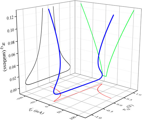
The sets of loci plotted in Figures 7A, C, D are 2D projections of the steady-state loci $(x_Q,i_Q,v_Q)$ in the 3D state space. Figure 8 shows the locus of $(x_Q,i_Q,v_Q)$ calculated for the midsize ${\text{VO}}_2$ device ($r_{\text{ch}}=36$ nm and $L_{\text{ch}}=50$ nm). It resembles a twisted handle of a binder clip. The two open legs of the clip are rotated out of the plane defined by the looped clip head. Figure 9 provides a zoomed-in view of Figure 8 to visualize the low-current region of the same $(x_Q,i_Q,v_Q)$ locus, allowing its 2D projections onto the $(i,x)$, $(v,x)$, and $(i,v)$ planes to be directly compared with the loci shown in Figures 7A, C, D, respectively.

Figure 8

Figure 8. Locus of fixed points $(x_Q,i_Q,v_Q)$ in the 3D state space of $(x,i,v)$ calculated for the midsize ${\text{VO}}_2$ Mott memristor (blue line) and its 2D projections (green, black, and red lines).

Figure 9

Figure 9. Zoomed-in view of Figure 8 to visualize the low-current region of the fixed-point locus $(x_Q,i_Q,v_Q)$ calculated for the midsize ${\text{VO}}_2$ Mott memristor. Its 2D projections (green, black, and red lines) can be compared with the loci $i_Q(x_Q)$, $v_Q(x_Q)$, and $(i_Q,v_Q)$ shown in Figure 7.

4 Local analysis of an isolated Mott memristor

4.1 Linearization and small-signal analysis

Chua’s LA theory outlines an algorithmic analysis procedure on nonlinear dynamical electronic circuits using equivalent linearized circuits (Chua, 2005). The linearized LA analysis examines the locus of fixed points of the composite circuit, the fluctuations around these fixed points, and their Laplace transforms. To explore the complex phenomena of nonlinear dynamical circuits, one can simply apply the LA criteria to access the locally active parameter domain rather than applying a time-consuming trial-and-error search in the parameter space. A good illustration of this procedure is the memristive HH axon circuit model (Chua et al., 2012). In this study, we apply the local linearization analysis and the LA theory to an isolated ${\text{VO}}_2$ Mott memristor to gain insights into its behavior near fixed points.

4.1.1 Linearization around a fixed point

Considering a fixed point $Q$ with a coordinate $(x_Q,i_Q)$ on the steady-state locus of an isolated Mott memristor, one can expand voltage $v$ at the fixed point $(x_Q,i_Q)$ in a Taylor series:

$v\left(x_Q+\delta x,i_Q+\delta i\right)=v_Q+i_Q{R}_{\text{ch}}^{\prime }\left(x_Q\right)\delta x+R_{\text{ch}}\left(x_Q\right)\delta i+\text{h.o.t.},(10)$

where $R_{\text{ch}}^{\prime }(x_Q)\triangleq \frac{d{R}_{\text{ch}}}{dx}{|}_Q$ and $\text{h.o.t.}$ denotes higher-order terms in $\delta x$ and $\delta i$. Neglecting $\text{h.o.t.}$, in Equation 10 we obtain a linear equation as follows:

$\delta v=i_Q{R}_{\text{ch}}^{\prime }\left(x_Q\right)\delta x+R_{\text{ch}}\left(x_Q\right)\delta i=a_{11}\left(Q\right)\delta x+a_{12}\left(Q\right)\delta i,(11)$

where coefficients $a_{11}(Q)\triangleq i_Q{R}_{\text{ch}}^{\prime }(x_Q)$ and $a_{12}(Q)\triangleq R_{\text{ch}}(x_Q)$. Similarly, the kinetic function $f_x(x,i)$ can be expanded at the fixed point $(x_Q,i_Q)$ in a Taylor series as follows:

$\begin{array}{ll}\hfill f_x\left(x_Q+\delta x,i_Q+\delta i\right)& =f_x\left(x_Q,i_Q\right)+\frac{\partial f_x\left(x,i\right)}{\partial x}{|}_Q\delta x\hfill \\ \hfill & +\frac{\partial f_x\left(x,i\right)}{\partial i}{|}_Q\delta i+\text{h.o.t.}.\hfill \end{array}(12)$

Note that $f_x(x_Q,i_Q)=0$ since it is a fixed point $(x_Q,i_Q)$ on the steady-state locus. Neglecting $\text{h.o.t.}$, in Equation 12 we can recast the nonlinear state equation $\frac{dx}{dt}=f_x(x,i)$ into the following linear differential equation:

$\frac{d}{dt}\left(\delta x\right)=\frac{\partial f_x\left(x,i\right)}{\partial x}{|}_Q\delta x+\frac{\partial f_x\left(x,i\right)}{\partial i}{|}_Q\delta i=b_{11}\left(Q\right)\delta x+b_{12}\left(Q\right)\delta i,(13)$

where coefficients $b_{11}(Q)\triangleq \frac{\partial f_x(x,i)}{\partial x}{|}_Q$ and $b_{12}(Q)\triangleq \frac{\partial f_x(x,i)}{\partial i}{|}_Q$. Applying Equations 2, 3, one can easily obtain the expressions for the following three linear-term coefficients:

$a_{11}\left(Q\right)=-\frac{2B{i}_Q{x}_Q}{A{\left(1+B{x}_Q^2\right)}^2},(14)$

$a_{12}\left(Q\right)=R_{\text{ch}}\left(x_Q\right)=\frac{1}{A\left(1+B{x}_Q^2\right)},(15)$

$b_{12}\left(Q\right)=\frac{4x_Q{\left(\ln x_Q\right)}^2{i}_Q}{DA\left(1+B{x}_Q^2\right)\left[1-x_Q^2+2x_Q^2\ln x_Q+2E{\left(x_Q\ln x_Q\right)}^2\right]}.(16)$

To obtain the expression for $b_{11}(Q)$, we rewrite $f_x(x,i)$ as $f_x(x,i)=\frac{i^{2}X(x)+Y(x)}{Z(x)}$, where the three auxiliary functions are defined as $X(x)=\frac{2x{(\ln x)}^2}{A(1+B{x}^2)}$, $Y(x)=2Cx\ln x$, and $Z(x)=D[1-x^2+2x^2\ln x+2E{(x\ln x)}^2]$. Applying the quotient rule $\frac{d}{dx}\frac{X(x)}{Z(x)}=\frac{X^{\prime }(x)Z(x)-X(x)Z^{\prime }(x)}{Z{(x)}^2}$, we obtain

$\begin{array}{ll}\hfill b_{11}\left(Q\right)& =i_Q^2{\left.\frac{X^{\prime }\left(x\right)Z\left(x\right)-X\left(x\right)Z^{\prime }\left(x\right)}{Z{\left(x\right)}^2}\right|}_Q\hfill \\ \hfill & +{\left.\frac{Y^{\prime }\left(x\right)Z\left(x\right)-Y\left(x\right)Z^{\prime }\left(x\right)}{Z{\left(x\right)}^2}\right|}_Q.\hfill \end{array}(17)$

The formulas for $X^{\prime }(x)\triangleq \frac{dX(x)}{dx}$, $Y^{\prime }(x)\triangleq \frac{dY(x)}{dx}$, and $Z^{\prime }(x)\triangleq \frac{dZ(x)}{dx}$ are $X^{\prime }(x)=\frac{2\ln x\left(2B{x}^2-B{x}^2\ln x+\ln x+2\right)}{A{\left(1+B{x}^2\right)}^2}$, $Y^{\prime }(x)=2C(\ln x+1)$, and $Z^{\prime }(x)=4Dx\ln x[1+E(\ln x+1)]$, respectively.

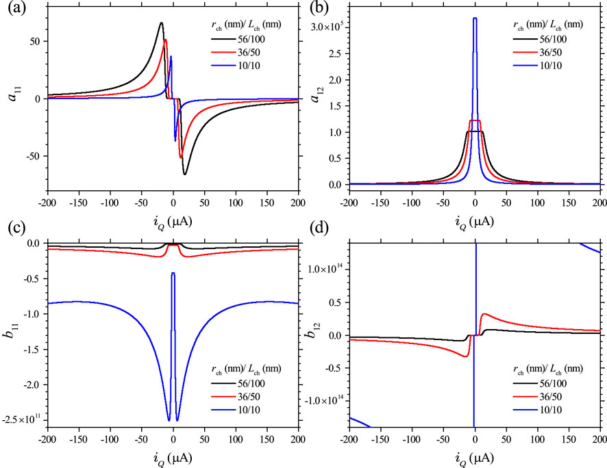
Figures 10A–D show the plot of the current dependence of the linear-term coefficients $a_{11}$, $a_{12}$, $b_{11}$, and $b_{12}$, calculated using Equations 14–17 for three different ${\text{VO}}_2$ device sizes. They show that coefficients $a_{11}$ and $b_{12}$ are odd functions of the driving current, while coefficients $b_{11}$ and $a_{12}$ are even functions of the driving current. $a_{12}$ is the same as the memristance $R_{\text{ch}}$ and is always positive. In contrast, $b_{11}$ is always negative.

Figure 10

Figure 10. Current dependences of the linear-term coefficients (A) $a_{11}$, (B) $a_{12}$, (C) $b_{11}$, and (D) $b_{12}$ in the linearized expressions of voltage $v$ and the kinetic function $f_x(x,i)$ at a fixed point on the steady-state locus of three different-sized ${\text{VO}}_2$ Mott memristors, as labeled.

4.1.2 Complex-domain equivalent circuit

Many insights can be gained about an isolated Mott memristor through complex analysis. As the second step of the local analysis, we can obtain its complex-domain equivalent circuit using the linear Laplace transform $\widehat{f}(s)\triangleq {\int }_{0^{-}}^{\infty }f(t)e^{-st}dt$ that maps a function $f(t)$ in the time domain to a function $\widehat{f}(s)$ in the complex domain $\mathbb{C}$, whose elements are complex frequencies $s=\sigma +i\omega$. The complex domain is also known as the $s$-domain. One direct benefit of the Laplace transform is that it converts a differential equation into an algebraic equation.

Taking the Laplace transforms of Equations 11, 13, we obtain

$\widehat{v}\left(s\right)=a_{11}\left(Q\right)\widehat{x}\left(s\right)+a_{12}\left(Q\right)\widehat{i}\left(s\right),(18)$

$s\widehat{x}\left(s\right)=b_{11}\left(Q\right)\widehat{x}\left(s\right)+b_{12}\left(Q\right)\widehat{i}\left(s\right),(19)$

where $\widehat{x}(s)$, $\widehat{v}(s)$, and $\widehat{i}(s)$ denote the Laplace transforms of $\delta x(t)$, $\delta v(t)$, and $\delta i(t)$, respectively. Solving Equation 19 for $\widehat{x}(s)$, we obtain

$\widehat{x}\left(s\right)=\frac{b_{12}\left(Q\right)\widehat{i}\left(s\right)}{s-b_{11}\left(Q\right)}.(20)$

Substituting Equation 20 for $\widehat{x}(s)$ in Equation 18 and solving for the impedance function $Z(s;Q)\triangleq \widehat{v}(s)/\widehat{i}(s)$, we obtain the $s$-domain impedance function as follows:

$Z\left(s;Q\right)=\frac{a_{11}\left(Q\right)b_{12}\left(Q\right)}{s-b_{11}\left(Q\right)}+a_{12}\left(Q\right).(21)$

For a current-controlled memristor, the impedance function $Z(s;Q)$ in Equation 21 is the proper choice for its transfer function $H(s;Q)$. For a voltage-controlled memristor, admittance function $Y(s;Q)$ should be used. Chua pointed out that for a 1D system with just one-port state variable, its transfer function is also the scalar complexity function that forms the basis for the LA analysis (Chua, 2005). In Chua’s original LA formulations for reaction-diffusion systems, a port state variable of a “reaction” cell (equivalent to a lumped circuit element) interacts with the neighboring cells via an energy or matter flow such as diffusion. On the other hand, a non-port state variable describes isolated internal dynamics and does not interact with other cells. The concept of LA is defined concerning only port state variables. Clearly, the state variable $x$ in the Mott memristor model is a port state variable as it interacts with a coupled circuit element through the current (energy) flow.

Since the $s$-domain representation of a capacitor looks like a “resistance” $1/sC$, one can recast the small-signal impedance function $Z(s;Q)$ of a Mott memristor at a fixed point $Q$ as an equivalent circuit that consists of three virtual elements: a capacitor $C_1$ in parallel with a resistor $R_1$ and both of them in series with a second resistor $R_2$.

$Z\left(s;Q\right)=\frac{\left(\frac{1}{s{C}_1}\right)R_1}{\left(\frac{1}{s{C}_1}\right)+R_1}+R_2,(22)$

where

$R_1\triangleq -\frac{a_{11}\left(Q\right)b_{12}\left(Q\right)}{b_{11}\left(Q\right)},(23)$

$R_2\triangleq a_{12}\left(Q\right)=R_{\text{ch}}\left(x_Q\right),(24)$

$C_1\triangleq \frac{1}{a_{11}\left(Q\right)b_{12}\left(Q\right)}.(25)$

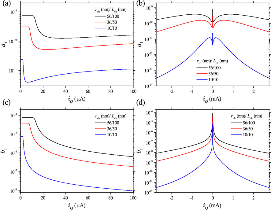
Figures 11A–C plot the current dependence of the three virtual circuit elements, namely, $R_1$, $R_2$, and $C_1$, calculated using Equations 23–25, respectively, for three different ${\text{VO}}_2$ device sizes. They are all even functions of the driving current, so we only plot the positive $x$-axis halves. The first thing to notice is that $R_1$ and $C_1$ stay negative at any current for all three device sizes calculated. In contrast, $R_2$ remains positive at any current. Note that $R_2$ is the same as $a_{12}$ and $R_{\text{ch}}(x_Q)$. Therefore, in the $s$-domain, a Mott memristor can be modeled as a nonlinear positive resistor in series with a composite reactive element consisting of a nonlinear negative capacitor and a nonlinear negative resistor placed in parallel. This small-signal equivalent circuit in the $s$-domain is shown in Figure 11B inset.

Figure 11

Figure 11. Current dependences of the three virtual circuit elements (A) $R_1$, (B) $R_2$, and (C) $C_1$ comprising the $s$-domain impedance function $Z(s;Q)$ at a fixed point on the steady-state $(i_Q,v_Q)$ loci of three different-sized ${\text{VO}}_2$ Mott memristors, as labeled. $R_1$ and $C_1$ remain negative at any current for all three device sizes. (B) The inset shows the small-signal equivalent circuit in the $s$-domain. (D) Current dependence for the sum of the two resistances $(R_1+R_2)$. $(R_1+R_2)$ turns negative as the current exceeds a size-dependent limit. (D) The inset shows that $(R_1+R_2)$ becomes positive again when the current exceeds a much larger size-dependent limit. These two current limits are identical with the critical currents $i_{c1}$ at the lower PDR to NDR and $i_{c2}$ at the NDR to upper PDR transitions on the steady-state $(i_Q,v_Q)$ loci, respectively (see Figure 7D and inset).

Since a negative capacitance value corresponds to a positive frequency-dependent inductive reactance, it indicates that a Mott memristor (or generally a current-controlled LAM) exhibits an apparent inductive reactance without involving a magnetic field. In physiology, an anomalous inductive reactance was observed as early as 1930s in voltage clamp measurements of the squid giant axon (Cole, 1941), but this perplexing phenomenon was not fully understood until Chua’s memristive formulation for the potassium and sodium ion channels (Chua et al., 2012).

Figure 11D shows the plots of the current dependence for the sum of the two resistances $(R_1+R_2)$. At small currents, $(R_1+R_2)$ is positive and remains nearly constant. As the current increases, $(R_1+R_2)$ decreases abruptly and becomes negative once the current exceeds a limit identical to the critical current $i_{c1}$ for the lower PDR to NDR transition on the steady-state $(i_Q,v_Q)$ loci (see Figure 7D) at 2.522 $\mathrm{\mu }$A, 9.077 $\mathrm{\mu }$A, and 14.122 $\mathrm{\mu }$A, respectively, for the three device sizes. The negative $(R_1+R_2)$ then starts to increase with the current. Inset of Figure 11D shows that $(R_1+R_2)$ becomes positive again as the current exceeds a much larger limit identical to the critical current $i_{c2}$ for the NDR to the upper PDR transition on the steady-state $(i_Q,v_Q)$ loci (see Figure 7D inset) at 269.77 $\mathrm{\mu }$A, 971.18 $\mathrm{\mu }$A, and 1510.73 $\mathrm{\mu }$A, respectively, for the same three devices. The one-to-one correspondence between the sign of $(R_1+R_2)$ and the sign of the slope on the steady-state $(i_Q,v_Q)$ loci indicates that the three-element equivalent circuit shown in Figure 11B inset is the proper small-signal representation of a Mott memristor in the $s$-domain.

4.2 Pole–zero diagram and Chua’s local activity theorem

4.2.1 Poles and zeros of the transfer function

For a dynamical system, the poles and zeros of its transfer function $H(s;Q)$ in the $s$-domain provide important insights into the system’s response without requiring a complete solution of the differential equations. The first step of pole–zero analysis is to rewrite the $s$-domain small-signal transfer function $H(s;Q)$ as a rational function of $s$, i.e., a ratio of two polynomials. For the case of a 1D current-controlled Mott memristor, both the denominator and numerator $s$ polynomials have a degree of $n=1$. Therefore, its impedance function $Z(s;Q)$ is written as follows:

$Z\left(s;Q\right)=\frac{b_{1}s+b_0}{a_{1}s+a_0},(26)$

where all the coefficients of $s$ polynomials in the denominator and numerator are real numbers. Using Equation 22, the expressions for these four coefficients are derived as follows:

$a_0=1,(27)$

$a_1=R_1{C}_1,(28)$

$b_0=R_1+R_2,(29)$

$b_1=R_1{R}_2{C}_1.(30)$

Since $a_0$ is a constant and $b_0=R_1+R_2$ has already been discussed (see Figure 11D), we only need to examine $a_1=R_1{C}_1$ and $b_1=R_1{R}_2{C}_1$. Both of them are even functions of the input current. Their dependence on current is plotted in Figure 12 for three different ${\text{VO}}_2$ device sizes.

Figure 12

Figure 12. Current dependences for two of the four $s$-polynomial coefficients: (A) $a_1$ (low-current part), (B) $a_1$ (wide range), (C) $b_1$ (low-current part), and (D) $b_1$ (wide range) in the rational function representation of the impedance function $Z(s;Q)$ at a fixed point on the steady-state $(i_Q,v_Q)$ locus of three different-sized ${\text{VO}}_2$ Mott memristors, as labeled. The other two coefficients are $a_0=1$ and $b_0=R_1+R_2$ (see Figure 11D).

A rational transfer function can be further rewritten in a factored or pole–zero form by expressing the $s$ polynomials in the denominator and numerator as products of linear factors. The roots of the denominator polynomial are the poles, and the roots of the numerator polynomials are the zeros. For any polynomial with real coefficients, its roots are either real or complex conjugate pairs.

For an isolated 1D Mott memristor, there is just one pole and one zero. To obtain the expressions for the zero and the pole of $Z(s;Q)$, Equation 26 is rewritten as follows:

$Z\left(s;Q\right)=\frac{k\left(s-z\right)}{\left(s-p\right)},(31)$

where $k=b_1/a_1=R_2$ is a positive real coefficient and $z$ and $p$ denote, respectively, the zero and the pole of $Z(s;Q)$. The expressions for $z$ and $p$ are as follows:

$z=-\frac{b_0}{b_1}=-\frac{R_1+R_2}{R_1{R}_2{C}_1},(32)$

$p=-\frac{a_0}{a_1}=-\frac{1}{R_1{C}_1}=b_{11}.(33)$

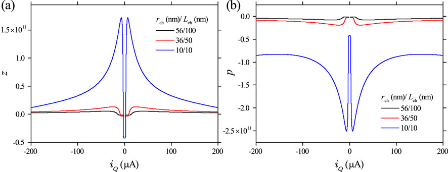
Figure 13 show the loci of the zero $z$ and the pole $p$ versus input current for three different ${\text{VO}}_2$ device sizes calculated using Equations 32, 33. It is conspicuous that both $z$ and $p$ are located on the real axis in the complex plane, and both are even functions of current. It may be noted that $p$ is already plotted in Figure 10C in the form of $b_{11}$. It is replotted in Figure 13B for a side-by-side comparison with $z$.

Figure 13

Figure 13. Current dependence of (A) the zero $z$ and (B) the pole $p$ of the $s$-domain impedance function $Z(s;Q)$ at a fixed point on the steady-state $(i_Q,v_Q)$ locus of a ${\text{VO}}_2$ Mott memristor, calculated for three different device sizes as labeled.

Since both the zero and the pole of $Z(s;Q)$ are located on the real axis, their signs can be examined to determine the local dynamical behaviors at a fixed point, as discussed in the next subsection. Generally speaking, for a 1D uncoupled Mott memristor, its pole $p$ (or $b_{11}$) remains negative at any current level. In contrast, its zero $z$ has two sign reversals at two distinctive input current levels. These characteristics are illustrated in Figure 14, which shows the current dependence of $p$ and $z$ of $Z(s;Q)$ calculated for the midsize ${\text{VO}}_2$ device ($r_{\text{ch}}=36$ nm and $L_{\text{ch}}=50$ nm).

Figure 14

Figure 14. Current dependence of the pole $p$ of $Z(s;Q)$ in (A, B) and the zero $z$ in (C, D) for the midsize ${\text{VO}}_2$ Mott memristor. $p$ remains negative at any current. For $z$, (C) $(-)\to (+)$ sign reversal is observed at 9.077 $\mathrm{\mu }$A, as indicated by a pair of nearby zeros $\{z1,z2\}$ with the opposite sign; (D) $(+)\to (-)$ sign reversal is observed at 971.18 $\mathrm{\mu }$A, as indicated by a pair of nearby zeros $\{z3,z4\}$ with the opposite sign. (E, F) Corresponding parts of the steady-state $(i_Q,v_Q)$ locus of the same device. The crossovers between the NDR region (red) and the lower and upper PDR regions (blue) at the local voltage extrema coincide with the sign reversals in $z$, as indicated by the locations of $\{Q_1,Q_2\}$ and $\{Q_3,Q_4\}$ pairs of fixed points on the $(i_Q,v_Q)$ locus.

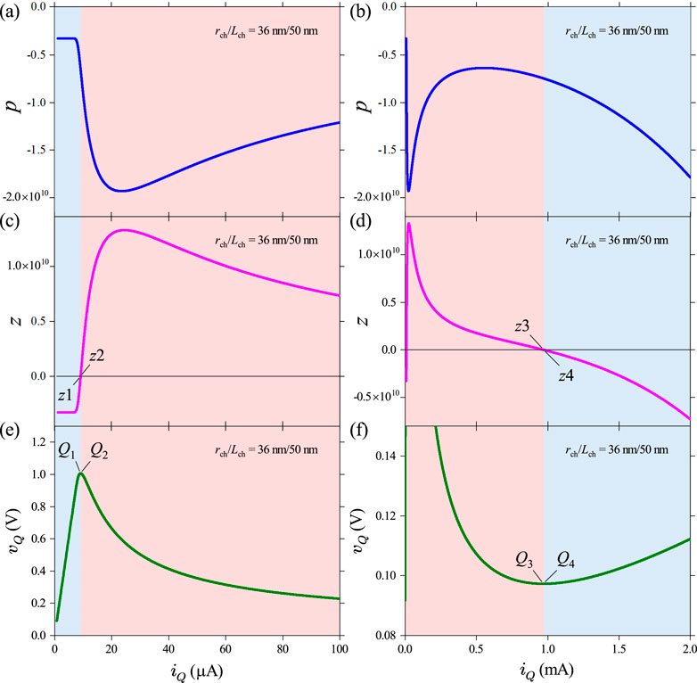
Figures 14A, B show the loci of $p(i_Q)$ for the low-current part (up to 100 $\mathrm{\mu }$A) and the broader range (up to 2 mA), respectively. $p$ exhibits a non-monotonic dependence on current, but the condition $p<0$ always holds true. Figure 14C shows that $z$ is initially negative at small currents, and then, it turns positive when the current is higher than $\approx$9.077 $\mathrm{\mu }$A, as indicated by a pair of nearby fixed points $\{Q_1,Q_2\}$ across zero. Their coordinates $[x_Q,i_Q,v_Q,\text{Re}(z)]$ are $[0.00566,9.075\mathrm{\mu }\text{A},1.007\text{\hspace{0.17em}V},-5.882\times 10^6]$ for $Q_1$ and $[0.00567,9.078\mathrm{\mu }\text{A},1.007\text{\hspace{0.17em}V},3.388\times 10^6]$ for $Q_2$, respectively. Figure 14D shows that $z$ becomes negative again if the current exceeds $\approx$971.18 $\mathrm{\mu }$A, as indicated by a pair of nearby fixed points $\{Q_3,Q_4\}$ across zero. Their coordinates are $[0.60628,971.171\mathrm{\mu }\text{A},0.097\text{\hspace{0.17em}V},3.854\times 10^4]$ for $Q_3$ and $[0.60629,971.203\mathrm{\mu }\text{A},0.097\text{\hspace{0.17em}V},-8.477\times 10^4]$ for $Q_4$, respectively. The two critical currents corresponding to sign reversals in $z$ match exactly with those that delineate the NDR region from the lower and upper PDR regions on the steady-state $(i_Q,v_Q)$ locus of the same device, as shown in Figures 14E, F. The coincidences are confirmed by examining the locations of the same two pairs of nearby fixed points $\{Q_1,Q_2\}$ and $\{Q_3,Q_4\}$ on the $(i_Q,v_Q)$ locus.

4.2.2 Chua’s local activity theorem

Chua’s local analysis method established a practical set of criteria to classify the dynamics of an isolated or uncoupled nonlinear circuit element around its fixed points. To determine whether a linearized element is LP or locally active around a fixed point $Q=(x_Q,i_Q,v_Q)$, one must find out whether small input fluctuations lead to dissipating output fluctuations over time or, conversely, result in amplification. For the discussion, we choose the example of a 1D current-controlled memristor with current as the input and voltage as the output. Their roles are exchanged for a voltage-controlled memristor by duality. Mathematically, with a homogeneous initial condition $(\delta x(0),\delta i(0),\delta v(0))=\mathbf{0}$ (no fluctuation at $t=0$), a linearized element is LP if and only if (iff) the fluctuation energy integrated over time remains positive:

$\text{LP}\iff {\int }_0^{t^{\prime }}\delta i\left(t\right)\cdot \delta v\left(t\right)dt\ge 0,(34)$

for any finite time interval $t^{\prime }>0$. The uncoupled element is locally active at a fixed point $Q$ iff there exists an input fluctuation $\delta i(t)$ and a finite time $0<T<\infty$ such that the integrated fluctuation energy becomes negative. For a multidimensional element, the fluctuation power to be integrated is a scalar “dot” product between the two vectors $\delta \mathbf{i}(t)$ and $\delta \mathbf{v}(t)$.

However, it is not practical to inspect the time-domain integral in Equation 34 for all possible input fluctuations. By applying the Laplace transform, Chua derived a mathematically equivalent yet more practical formula for the local passivity theorem in the complex domain. For the 1D scalar case, the necessary and sufficient condition for an uncoupled 1D circuit element to be LP is that its complexity function or transfer function $H(s;Q)$ is a positive real (PR) function, which satisfies both (1) $\text{Im}[H(s;Q)]=0$ if $\text{Im}[s]=0$ and (2) $\text{Re}[H(s;Q)]\ge 0$ if $\text{Re}[s]\ge 0$. Condition (1) is always satisfied since $H(s;Q)$ is a rational function. Condition (2) means that the closed right half plane (RHP) of $s$ maps into the closed RHP of $H(s;Q)$. A simple example for a PR function is $H(s;Q)=a+bs+c{s}^{-1}$, where $a$, $b$, and $c\ge 0$.

Chua proved the following local passivity theorem as a practical test for the PR condition: an uncoupled 1D circuit element is LP at a fixed point iff all the following four criteria are satisfied.

i) $H(s;Q)$ has no poles in the open RHP $(\text{Re}(s)>0)$.

ii) $H(s;Q)$ has no higher-order poles (degree $n\ge 2$) on the imaginary axis (Im axis).

iii) If $H(s;Q)$ has a simple pole $s=i{\omega }_{\text{p}}$ on the Im axis, then the residue of $H(s;Q)$ at $i{\omega }_{\text{p}}$ must be a PR number.

iv) The Im axis (excluding poles) maps into the closed RHP of $H(s;Q)$, i.e., $\text{Re}[H(i\omega ;Q)]\ge 0$ for all $\omega \in (-\infty ,\infty )$, where $s=i\omega$ is not a pole.

The LA theorem is derived by negating any one of the abovementioned conditions. In other words, an uncoupled 1D circuit element is locally active at a fixed point iff any one of the following four criteria is satisfied.

i) $H(s;Q)$ has a pole in the open RHP $\text{Re}(s)>0$.

ii) $H(s;Q)$ has a higher-order pole (degree $n\ge 2$) on the Im axis.

iii) $H(s;Q)$ has a simple pole on the Im axis with negative-real or complex residue.

iv) At least some points on the Im axis map into the open left half plane (LHP) of $H(s;Q)$, i.e., $\text{Re}[H(i\omega ;Q)]<0$ for some $\omega \in (-\infty ,\infty )$.

For a system of higher dimensions, Chua proved a similar set of four test criteria for LA, where the complexity function $H(s;Q)$ for an 1D element is replaced by the complexity matrix for a multidimensional element.

As explained by Brown et al. (2022b), the local stability of a fixed point is a property that is independent of the local activity of dynamics around it. Near a fixed point, an isolated memristor may have four possible combinations of local stability and local activity properties that can lead to persistent or decaying dynamics. Since the condition of being both LP and locally unstable is physically unrealizable, one generally only needs to consider three possible scenarios: LP and stable, locally active but asymptotically stable, which is termed as edge of chaos (EOC) by Chua, and locally active and unstable (LA$\backslash$EOC).

For a 1D uncoupled memristor, if its transfer function has a positive coefficient ($k>0$ in Equation 31), the classification of its dynamics around a fixed point is determined by the locations of the pole and zero of its transfer function in the complex plane, as specified below.

i) Locally passive $\iff$ pole in the open LHP $(\text{Re}(p)<0)$ and zero in the closed LHP $(\text{Re}(z)\le 0)$

ii) Edge of chaos $\iff$ pole in the open LHP $(\text{Re}(p)<0)$ and zero in the open RHP $(\text{Re}(z)>0)$

iii) Locally active but unstable $\iff$ pole in the closed RHP $(\text{Re}(p)\ge 0)$

Plots of $\text{Im}(p)$ versus $\text{Re}(p)$ and $\text{Im}(z)$ versus $\text{Re}(z)$, known as pole–zero diagram, thus, offer a graphical determination of local steady-state dynamics without resorting to time-domain integration.

As discussed previously, for a current-controlled Mott memristor both the pole and the zero are located on the real axis. The pole $p$ of its impedance function $Z(s;Q)$ is always in the open LHP $(\text{Re}(p)<0)$; therefore, it does not possess the LA$\backslash$EOC dynamics in (iii). On the other hand, the zero $z$ of $Z(s;Q)$ can reside in either the closed LHP or the open RHP, depending on the input current amplitude. Figure 14 shows that $\text{Re}(z)$ flips its sign twice depending on the input current, and the two sign reversals in $\text{Re}(z)$ coincide with the crossovers between the NDR region and the lower and upper PDR regions on the steady-state $(i_Q,v_Q)$ locus.

4.2.3 Pole–zero diagram

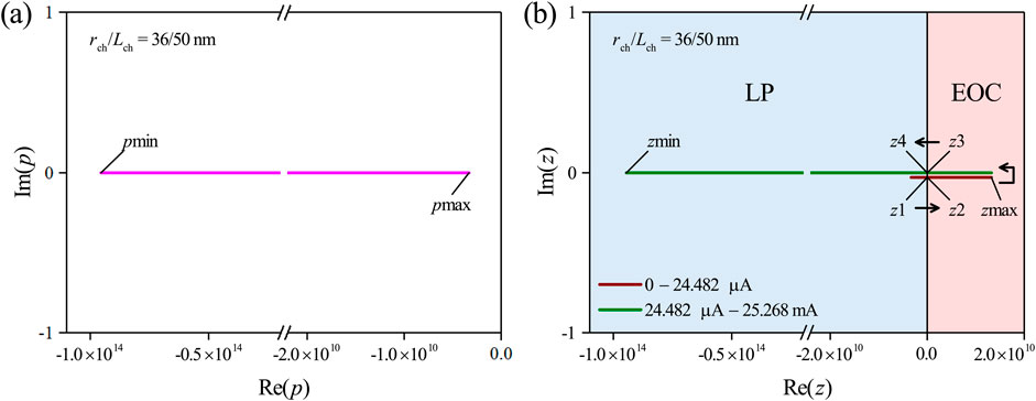
Figure 15 visualizes the evolution of $p$ and $z$ locations in the complex plane as functions of the input current for the current-controlled midsize ${\text{VO}}_2$ Mott memristor. Figure 15A shows that $\text{Re}(p)<0$ is always satisfied. The coordinates $[x_Q,i_Q,v_Q,\text{Re}(p)]$ for the minimal and maximal calculated values of $p$, labeled as $p_{\text{min}}$ and $p_{\text{max}}$, are $[0.998,25.268\text{\hspace{0.17em}mA},0.935\text{\hspace{0.17em}V},-9.543\times 10^{13}]$ and $[1\times 10^{-145},1.074\mathrm{\mu }\text{A},0.132\text{\hspace{0.17em}V},-3.273\times 10^9]$, respectively. As may be noted, $p_{\text{min}}$ and $p_{\text{max}}$ in our calculations are not the actual bounds of $p$ since $x_Q$ can approach to its asymptotes 0 and 1 very closely but will never reach them.

Figure 15

Figure 15. Locations of (A) the pole $p$ and (B) the zero $z$ in the complex plane as functions of the input current, calculated for the midsize ${\text{VO}}_2$ Mott memristor. Both $p$ and $z$ are located on the real axis. $p$ remains in the LHP, with its minimal and maximal calculated values indicated by $p_{\text{min}}$ and $p_{\text{max}}$, respectively. $z$ is located in the LHP at $i_Q=0$ and shifts to the right with current, crossing the imaginary axis into the RHP at 9.077 $\mathrm{\mu }$A, as indicated by $\{z1,z2\}$. It continues to shift to the right until reaching $z_{\text{max}}$ at 24.482 $\mathrm{\mu }$A, then shifts to the left with current, and reenters LHP at 971.18 $\mathrm{\mu }$A, as indicated by $\{z3,z4\}$. The minimum of $z$ is represented as $z_{\text{min}}$. The part of $z$ locus between 0 and 24.482 $\mathrm{\mu }$A (brown) is shifted vertically for clarity. The LP and EOC regions are highlighted by blue and red colors, respectively.

Figure 15B shows that the zero $z$ is located in the LHP at zero current, and it shifts to the right as the current increases. $z$ crosses the Im axis into the RHP at a critical current of 9.077 $\mathrm{\mu }$A, as indicated by a pair of nearby fixed points $\{z1,z2\}$ on the opposite side of the Im axis (the same ones as shown in Figure 14). $z$ continues shifting to the right with current until it reaches a maximum value at $z_{\text{max}}$ with a coordinate of $[0.03549,24.482\mathrm{\mu }\text{A},0.578\text{\hspace{0.17em}V},1.327\times 10^{10}]$. Then, it reverses course and shifts to the left with current. $z$ crosses the Im axis again and returns to the LHP at a second critical current of 971.18 $\mathrm{\mu }$A, as indicated by a pair of nearby fixed points $\{z3,z4\}$ on the opposite side of the Im axis (the same ones as shown in Figure 14). Continuously increasing the current will drive $x_Q$ asymptotically toward 1 and further decrease $z$. We stop the calculation at $z_{\text{min}}$ with a coordinate of $[0.998,25.268\text{\hspace{0.17em}mA},0.935\text{\hspace{0.17em}V},-9.467\times 10^{13}]$. We use the same blue and red colors, as shown in Figure 14 to highlight the LP and EOC regions, respectively.

Applying the pole–zero diagram LA criteria specified above, we conclude that an uncoupled 1D Mott memristor at a fixed point either belongs to the LP class or the EOC class but can never belong to the LA$\backslash$EOC class. For the midsize ${\text{VO}}_2$ device, the LP $\to$ EOC transition occurs at $(x_Q,i_Q,v_Q)\approx (0.00567,9.076\mathrm{\mu }\text{A},1.007\text{\hspace{0.17em}V})$. The EOC $\to$ LP transition occurs at $(x_Q,i_Q,v_Q)\approx (0.60629,971.2\mathrm{\mu }\text{A},0.0973\text{\hspace{0.17em}V})$.

4.3 Frequency response

An important question arises: for an uncoupled 1D Mott memristor that is current-biased in the EOC region (which coincides with its NDR region), will it remain to be locally active, capable of amplifying a small sinusoidal input fluctuation at arbitrarily high frequencies? Otherwise, is there a finite upper limit for the input fluctuation frequency, beyond which the element can no longer provide an AC signal gain? In this section, we shift the small-signal analysis to the frequency domain, which allows us to apply the fourth criterion in Chua’s LA theorem to answers these questions.

For dynamical systems, it is useful to study the system’s frequency response. In small-signal analysis, this is performed by applying a single-frequency sinusoidal fluctuation of current input $i(t)=I\sin \omega t$ with an angular frequency $\omega =2\pi f$, where $f$ is the frequency of the sine wave. The amplitude $I\ll 1$ is very small to satisfy the small-signal condition. For a 1D Mott memristor at a fixed point $Q$, substituting $s=i\omega$ for the complex frequency $s$ in the small-signal impedance $Z(s;Q)$ in Equation 26 and rearranging into its real and imaginary parts, we obtain

$Z\left(i\omega ;Q\right)=\left[\frac{a_0{b}_0+a_1{b}_1{\omega }^2}{a_0^2+a_1^2{\omega }^2}\right]+i\left[\frac{\left(a_0{b}_1-a_1{b}_0\right)\omega }{a_0^2+a_1^2{\omega }^2}\right].(35)$

The functions $\text{Re}Z(i\omega ;Q)$ and $\text{Im}Z(i\omega ;Q)$ are the real and imaginary parts of the frequency response, respectively; these are expressed in terms of the small-signal impedance $Z(i\omega ;Q)$, both of which are rational functions of $\omega$:

$\text{Re}Z\left(i\omega ;Q\right)=\frac{a_0{b}_0+a_1{b}_1{\omega }^2}{a_0^2+a_1^2{\omega }^2},(36)$

$\text{Im}Z\left(i\omega ;Q\right)=\frac{\left(a_0{b}_1-a_1{b}_0\right)\omega }{a_0^2+a_1^2{\omega }^2},(37)$

where the coefficients $a_0$, $a_1$, $b_0$, and $b_1$ are provided in Equations 27–30.

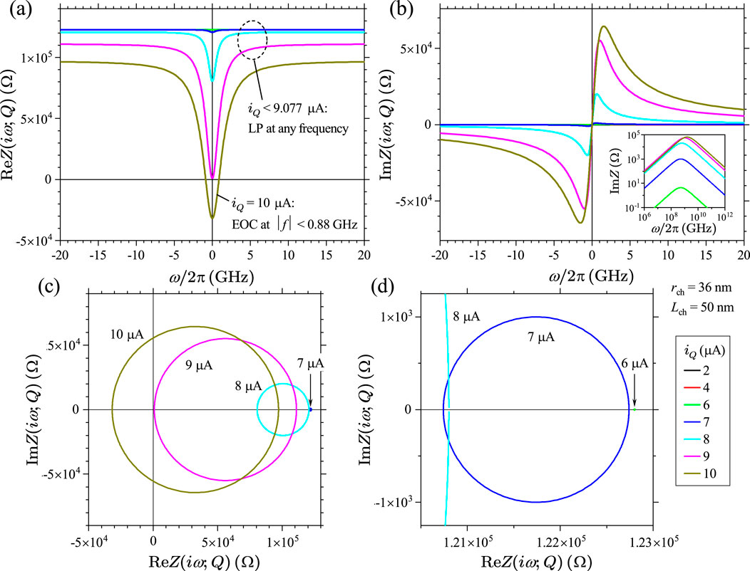
Figures 16A, B show the plot of the frequency dependence of $\text{Re}Z(i\omega ;Q)$ and $\text{Im}Z(i\omega ;Q)$ (also referred to as Re$Z$ and Im$Z$, respectively, hereafter) at different steady-state current levels between 2 $\mathrm{\mu }$A and 10 $\mathrm{\mu }$A for the midsize ${\text{VO}}_2$ Mott memristor calculated using Equations 36, 37. We replaced angular frequency $\omega$ with frequency $f$ as the $x$-axis for engineering convenience. Notice that positive and negative frequencies refer to the opposite directions of rotation for the complex exponential $e^{i\omega t}$ vector in the complex plane. Re$Z$ is an even function of frequency, while Im$Z$ is an odd function of frequency. At small currents, Re$Z$ is in the order of $10^5\mathrm{\Omega }$ and shows very weak frequency dependence. Increasing current will “pull” it toward the negative direction and develop a dip centered at zero frequency. The higher the current is, the stronger the frequency dependence becomes.

Figure 16

Figure 16. Small-signal impedance $Z(i\omega ;Q)$ frequency response of the midsize ${\text{VO}}_2$ Mott memristor biased at constant steady-state currents in the range of 2 $\mathrm{\mu }$A to 10 $\mathrm{\mu }$A. (A) $\text{Re}Z(i\omega ;Q)$ vs $\omega /2\pi$ (in GHz). At $i_Q<9.077$ $\mathrm{\mu }$A, Re$Z>0$ at any frequency, and the memristor remains LP. At $i_Q=10$ $\mathrm{\mu }$A, an EOC region exists with Re$Z<0$ at $\left|f\right|<0.88$ GHz. (B) $\text{Im}Z(i\omega ;Q)$ vs $\omega /2\pi$. Inset is a part of the same figure plotted in log–log scale. (C) Nyquist plot of $\text{Im}Z(i\omega ;Q)$ vs $\text{Re}Z(i\omega ;Q)$. (D) Zoomed portion of (C) reveals the loci at smaller currents.

Frequency response of Re$Z$ shows a dramatic change as the current increases from 9 $\mathrm{\mu }$A to 10 $\mathrm{\mu }$A. From the pole–zero diagram analysis, we already know that for the midsize ${\text{VO}}_2$ Mott memristor, the critical current at the LP (lower PDR) to EOC (NDR) crossover is $i_{c1}\approx 9.077$ $\mathrm{\mu }$A. At $i_Q=9$ $\mathrm{\mu }$A, Re$Z$ still remains positive at any frequency, but its minimum at zero frequency is very close to the origin. At $i_Q=10$ $\mathrm{\mu }$A, Re$Z$ turns negative at frequencies lower than the limit $\left|f_{\text{max}}\right|\approx 0.88$ GHz, indicating that the element is locally active within certain frequency upper bound. This $(+)\to (-)$ sign reversal in Re$Z$ is yet another hallmark of the LP $\to$ EOC transition and provides new information on the boundary of the EOC region in the frequency domain.

The value of $f_{\text{max}}$ can be derived from Chua’s fourth LA criterion. For an uncoupled 1D current-driven memristor in the frequency domain, $\text{Re}Z(i\omega ;Q)<0$; for some finite angular frequencies, $\omega \in (-\infty ,\infty )$ is a sufficient condition for it to be LA. From Equation 35, this means $a_0{b}_0+a_1{b}_1{\omega }^2<0$ or ${\omega }^2<\frac{-a_0{b}_0}{a_1{b}_1}$. Therefore, a 1D uncoupled Mott memristor is locally active if the angular frequency is lower than the upper bound specified as follows:

$\left|\omega \right|<{\omega }_{\text{max}}=\sqrt{\frac{-a_0{b}_0}{a_1{b}_1}},(38)$

which also requires that $\frac{a_0{b}_0}{a_1{b}_1}<0$ so that ${\omega }_{\text{max}}$ in Equation 38 is a real number.

At small currents, Im$Z$ is both very small and shows very weak frequency dependence. As the current increases, its amplitude and frequency dependence become more pronounced. The amplitude of Im$Z$ first increases rapidly with frequency before reaching a peak at a characteristic frequency $f_{\text{p}}$, and then, it decreases with frequency and asymptotically approaches the $x$-axis. $\left|f_{\text{p}}\right|$ increases with the current and reaches 1.51 GHz at $i_Q=10$ $\mathrm{\mu }$A. Inset of Figure 16B presents the same frequency dependence of Im$Z$ plotted on a log–log scale, which shows that Im$Z$ is proportional to the frequency for $\left|f\right|<\left|f_{\text{p}}\right|$ and inversely proportional to the frequency for $\left|f\right|>\left|f_{\text{p}}\right|$.

4.3.1 Nyquist plot

It is instructive to plot the locus of $\text{Im}Z(i\omega ;Q)$ vs. $\text{Re}Z(i\omega ;Q)$ in Cartesian coordinates, with $\omega$ indicated as a parameter. Such a parametric plot is called a Nyquist plot, a graphical technique used to provide insights into the stability of a dynamical system.

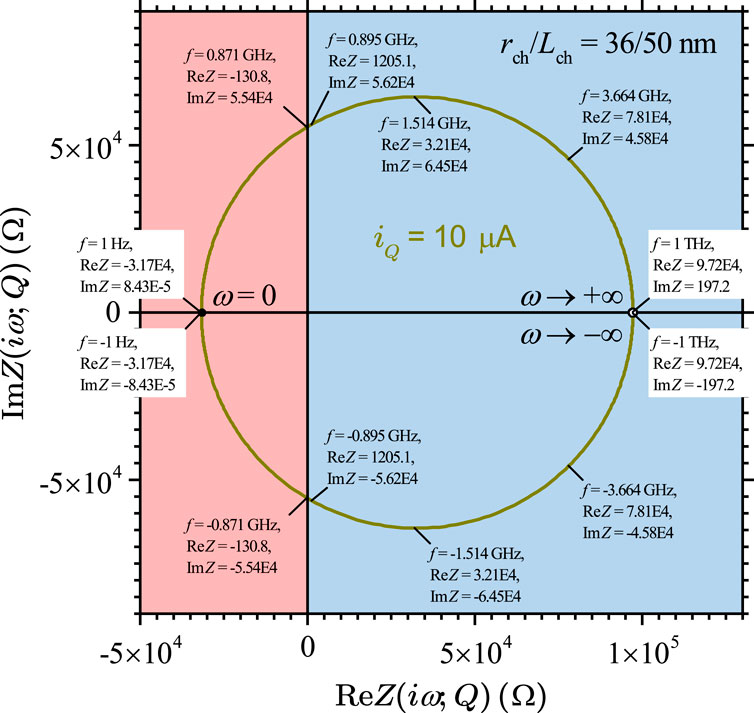
Figure 16C shows the loci of the Nyquist plot for the same ${\text{VO}}_2$ device, as shown in Figures 16A, B. Figure 16D presents a zoomed-in portion of it to reveal those much smaller loci at $i_Q\le 7$ $\mathrm{\mu }$A. Ostensibly, the locus of small-signal $\text{Im}Z(i\omega ;Q)$ vs $\text{Re}Z(i\omega ;Q)$ at a finite steady-state current appears to be a circle centered on the $x$-axis. Increasing the current will inflate the radius of the circle and move its center toward the negative direction. Points in the upper half-plane correspond to positive frequencies, and those in the lower half-plane correspond to negative frequencies. Increasing the frequency modulus will move a point in the right direction along the upper or lower arm of the locus. A closer look reveals that the left half of the locus intersects the $x$-axis at zero frequency. For the right half, the distance between the locus and the $x$-axis approaches 0 as $\left|f\right|\to \infty$, but there is no intersection at any finite frequency. In other words, the $x$-axis is a horizontal asymptote for the right half of the locus. Therefore, the locus of $\text{Im}Z(i\omega ;Q)$ vs $\text{Re}Z(i\omega ;Q)$is actually an open set of points rather than a closed loop. At $i_Q\approx 9.077$ $\mathrm{\mu }$A, the locus crosses the $y$-axis into the LHP, as illustrated by the two loci at 9 $\mathrm{\mu }$A and 10 $\mathrm{\mu }$A. Therefore, the Nyquist plot provides another visualization of the LP $\to$ EOC transition as the steady-state current increases.

Figure 17 is an annotated Nyquist plot for the Im$Z$ vs Re$Z$ locus of the same ${\text{VO}}_2$ device at $i_Q=10$ $\mathrm{\mu }$A, highlighting several key points on the locus. We use the same blue and red colors, as shown in Figures 14, 15 to represent the LP and EOC regions, respectively. Clearly, the lower half of the locus is a reflection of the upper half over the $x$-axis, by negating the values of Im$Z$ and frequency at the same Re$Z$ value. The solid dot $(•)$ at Re$Z\approx -3.17\times 10^4$ represents the $x$-intercept of the locus at zero frequency, as indicated by a pair of nearby points at $f=1$ Hz and $f=-1$ Hz. The open circle $(◦)$ at Re$Z\approx 9.72\times 10^4$ represents the $x$-asymptote of the locus as $\left|f\right|\to \infty$, as indicated by a pair of nearby points at $f=1$ THz and $f=-1$ THz. The two pairs of points at $f=\pm 0.871$ GHz and $f=\pm 0.895$ GHz indicate the crossover from the EOC (red) region to the LP (blue) region as frequency exceeds 0.88 GHz.

Figure 17

Figure 17. Nyquist plot of $\text{Im}Z(i\omega ;Q)$ vs $\text{Re}Z(i\omega ;Q)$ of the midsize ${\text{VO}}_2$ Mott memristor at a constant steady-state current $i_Q=10$ $\mathrm{\mu }$A. The LP and EOC regions are highlighted in blue and red colors, respectively.

4.3.2 Frequency-domain equivalent circuit

The frequency-domain equivalent circuit of an isolated Mott memristor can be readily obtained by substituting $a_0$, $a_1$, $b_0$, and $b_1$ in Formula 35 of $Z(i\omega ;Q)$ with $R_1$, $R_2$, and $C_1$ using Equations 27–30. The real part of $Z(i\omega ;Q)$ as shown in Formula 36, now defined as the frequency-domain resistance function, takes the form of

$R_{\omega }\left(\omega ,Q\right)\triangleq \text{Re}Z\left(i\omega ;Q\right)=\frac{\left(R_1+R_2\right)+{\left(R_1{C}_1\right)}^2{R}_2{\omega }^2}{1+{\left(R_1{C}_1\right)}^2{\omega }^2},(39)$

which can be further rewritten by replacing $C_1$ with $-1/b_{11}{R}_1$ using Equation 33

$R_{\omega }\left(\omega ,Q\right)=\frac{b_{11}^2\left(R_1+R_2\right)+R_2{\omega }^2}{b_{11}^2+{\omega }^2}.(40)$

The sign of $R_{\omega }(\omega ,Q)$ can be either positive or negative, depending on the $(\omega ,Q)$ coordinate. $R_{\omega }(\omega ,Q)\ge 0$ maps to the LP region, and $R_{\omega }(\omega ,Q)<0$ maps to the EOC region. The angular frequency in Formula 38 to satisfy Chua’s fourth LA criterion now becomes

$\left|\omega \right|<{\omega }_{\text{max}}=-b_{11}\sqrt{\frac{-\left(R_1+R_2\right)}{R_1}}.(41)$

Since the memristance $R_2$ is always positive, this indicates that $(R_1+R_2)$ must be negative for ${\omega }_{\text{max}}$ to be a real number. From the previous discussion of Figure 11D, $(R_1+R_2)<0$ maps into the NDR (EOC) region on the steady-state $(i_Q,v_Q)$ locus.

We now look at the imaginary part of $Z(i\omega ;Q)$. By substituting $a_0$, $a_1$, $b_0$, and $b_1$ in Formula 37 of $\text{Im}Z(i\omega ;Q)$ with $R_1$, $R_2$, and $C_1$, we rewrite $\text{Im}Z(i\omega ;Q)$ as

$\text{Im}Z\left(i\omega ;Q\right)\triangleq L_{\omega }\left(\omega ,Q\right)\omega =\left[\frac{-R_1^2{C}_1}{1+{\left(R_1{C}_1\right)}^2{\omega }^2}\right]\omega ,(42)$

where $L_{\omega }(\omega ,Q)$ is defined as the frequency-domain inductance function. Evidently, the sign of $L_{\omega }(\omega ,Q)$ is determined by the sign of $C_1$. Since $C_1$ remains negative at any fixed point $Q$ (see discussion on Figure 11C), $L_{\omega }(\omega ,Q)$ is always positive, regardless of the location of $Q$ in the LP or EOC region. Therefore, the frequency-domain reactance of an isolated Mott memristor is always inductive, causing its voltage output to lead a sinusoidal current input in phase. $\text{Im}Z(i\omega ;Q)$ can be further rewritten by replacing $C_1$ with $-1/b_{11}{R}_1$ as follows:

$L_{\omega }\left(\omega ,Q\right)\omega =\left(\frac{b_{11}{R}_1}{b_{11}^2+{\omega }^2}\right)\omega .(43)$

Finally, the frequency-domain small-signal impedance function is expressed as

$Z\left(i\omega ;Q\right)=R_{\omega }\left(\omega ,Q\right)+i{L}_{\omega }\left(\omega ,Q\right)\omega .(44)$

Through Equations 39–44, we conclude that in the frequency domain, an uncoupled Mott memristor can be considered a positive inductor in series with a resistor that is negative up to a certain maximum frequency (the EOC region) and positive beyond it (the LP region) (Liang et al., 2022).

4.3.3 Phase diagram for complexity

The fourth criterion in Chua’s LA theorem states that a negative real part of the complexity function of an uncoupled 1D circuit element at some finite frequencies is a sufficient condition for it to be locally active. For a current-driven memristor, its complexity function is the impedance function $Z(i\omega ;Q)$. Since $Z(i\omega ;Q)$ depends on both the angular frequency $\omega$ and the steady-state current $i_Q$, plotting Re$Z$ as a color scale with current and frequency as the $(x,y)$ coordinate provides a visualization of the LP and EOC regions in the operating parameter space. The $\text{Re}Z=0$ contour outlines the border between these regions. One could refer to such a 2D graphical representation of Re$Z$ a phase diagram for complexity.

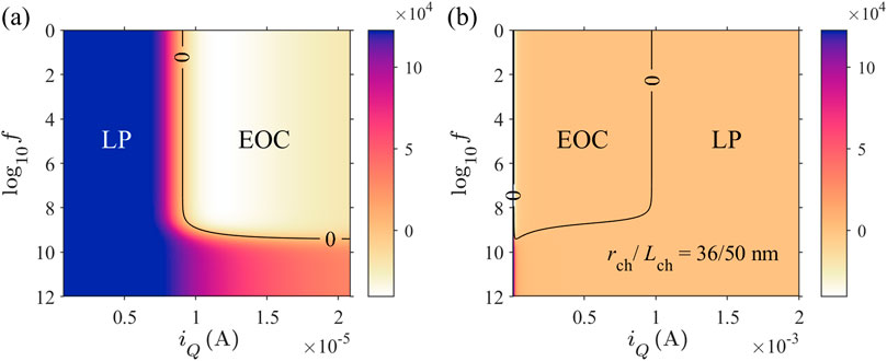
Figure 18 shows the plot of the 2D color-scale map of $\text{Re}Z(i_Q,f)$ for the midsize ${\text{VO}}_2$ Mott memristor. Figure 18A presents the low-current region, plotted up to 20.8 $\mathrm{\mu }$A. It shows that at lower frequencies, the LP $\to$ EOC transition occurs at a nearly frequency-independent critical current $i_{c1}\approx 9.077$ $\mathrm{\mu }$A, as indicated by an almost vertical $\text{Re}Z=0$ contour. At frequencies higher than $\sim$0.88 GHz, the critical current increases drastically, and consequently, the direction of the $\text{Re}Z=0$ contour turns almost parallel to the current axis. Figure 18B shows the same color-scale Re$Z$ map, with a much wider current range up to 2 mA, revealing an EOC $\to$ LP transition that occurs at a nearly constant critical current $i_{c2}\approx 971.18$ $\mathrm{\mu }$A at low frequencies. The direction of the $\text{Re}Z=0$ contour shows a similar crossover from nearly vertical at frequencies lower than $\sim$0.88 GHz to almost horizontal at higher frequencies.

Figure 18

Figure 18. 2D color-scale map of $\text{Re}Z(i_Q,f)$ for the midsize ${\text{VO}}_2$ Mott memristor as a visualization of the LP and EOC regions in the frequency and current parameter space, showing (A) its low-current region up to $i_Q=20.8$ $\mathrm{\mu }$A and (B) a wide-range map plotted up to $i_Q=2$ mA. Frequencies are plotted on a logarithmic scale.

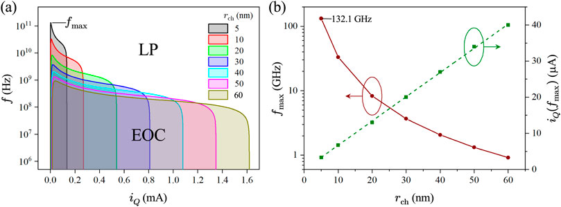
To understand the scaling trend of the local activity region versus device size, we plotted the 2D color-scale map of $\text{Re}Z(i_Q,f)$ for ${\text{VO}}_2$ Mott memristors with different combinations of $r_{\text{ch}}$ and $L_{\text{ch}}$ sizes. Figure 19 shows the main results of this analysis. We found that Re$Z$ is independent of the ${\text{VO}}_2$ channel length $L_{\text{ch}}$. This is not unexpected since the ${\text{VO}}_2$ compact model is essentially 2D in nature. Figure 19A presents a zoomed-in view of the $\text{Re}Z=0$ contours for ${\text{VO}}_2$ devices with $r_{\text{ch}}$ in the range of 5–60 nm. The shaded area under each contour is the EOC region that satisfies $\text{Re}Z(i_Q,f)<0$. The apex of each contour corresponds to the maximum frequency $f_{\text{max}}$ at which the device remains locally active. Figure 19B shows that $f_{\text{max}}$ increases super-exponentially as the ${\text{VO}}_2$ channel radius $r_{\text{ch}}$ shrinks. For a ${\text{VO}}_2$ device with $r_{\text{ch}}$ as small as 5 nm, $f_{\text{max}}$ reaches as high as 132.1 GHz. This favorable device scaling enhances the operational bandwidth for using Mott memristors as locally active components. It also reveals that the steady-state current at $f_{\text{max}}$ is directly proportional to the radius of the conduction channel $r_{\text{ch}}$.

Figure 19

Figure 19. (A) Zoomed-in view of the $\text{Re}Z=0$ contours for ${\text{VO}}_2$ Mott memristors with channel radius $r_{\text{ch}}$ in the range of 5 nm–60 nm. Shaded areas under the contours are the EOC regions, where $\text{Re}Z(i_Q,f)<0$. The apex of each contour at $f=f_{\text{max}}$ shows the maximum frequency of the EOC region. (B) Scaling of $f_{\text{max}}$ (brown) and $i_Q(f_{\text{max}})$ (green) vs. $r_{\text{ch}}$. $f_{\text{max}}$ increases super-exponentially as $r_{\text{ch}}$ decreases. $i_Q(f_{\text{max}})$ scales linearly with $r_{\text{ch}}$. A linear regression (dashed line) yields a slope of $671\pm 3$ (A/m) and a coefficient of determination $R^2=0.99988$.

5 Local analysis of reactively coupled Mott memristors: two-dimensional relaxation oscillator

The topological constraint of an isolated 1D Mott memristor limits the dynamics it can exhibit, making damped or persistent oscillations impossible. However, this constraint may get lifted when the memristor is coupled to one or more reactive elements. The coupling may increase both the system’s dimension and the complexity of its dynamics. For continuous dynamical systems, the Poincaré–Bendixson theorem states that chaos only arises in three or more dimensions.

For simplicity, we will limit our discussions to 2D cases. Experimentally, it is difficult to characterize an isolated memristor without inadvertently coupling it to one or more reactive elements. On the other hand, such couplings introduce interesting phenomena such as self-excited persistent oscillations or stable limit cycles. Limit cycles belong to an important category of attractors, alongside fixed points. A nonlinear system consisting of a Mott memristor coupled with reactive elements may exhibit a local Hopf-like bifurcation. As a bifurcation parameter is varied, its local stability abruptly switches between a fixed point and a limit cycle around it. Persistent oscillations that arise out of Hopf-like bifurcations are well-studied in the Hodgkin–Huxley and FitzHugh–Nagumo models of biological nerve cells (Hastings, 1974; Troy, 1978; Rinzel and Miller, 1980; Dogaru and Chua, 1998), and they are relevant for the intriguing neuronal signaling phenomena such as firing action potentials. However, finding the limit cycle solutions for a dynamical system is generally a very difficult mathematical problem. The unsolved second part of Hilbert’s $16^{\text{th}}$ problem is a well-known example. The local analysis techniques that we have discussed so far are not sufficient, and one needs to resort to global nonlinear techniques such as nullcline analysis and Lyapunov stability theory. In this section, we apply local analysis to a simple example of a reactively coupled Mott memristor. In the next section, we take a cursory glance at global analysis using the same example to illustrate its usefulness.

5.1 Voltage-biased relaxation oscillator circuit

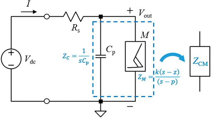
A voltage-biased Pearson–Anson (PA) relaxation oscillator circuit is a simple yet very useful example to illustrate the effect of such external couplings. As shown in Figure 20, if a Mott memristor $M$ is connected to a capacitor $C_{\text{p}}$ in parallel and both of them are connected to a resistor $R_{\text{s}}$ placed in series, then together they form a composite circuit, which can be represented as $\{(M\Vert C_{\text{p}})+R_{\text{s}}\}$. In practice, one may inadvertently form such a circuit when attempting to test an individual memristor device without explicitly connecting $C_{\text{p}}$ and $R_{\text{s}}$. $C_{\text{p}}$ may arise from the geometric capacitance between the two electrodes of a thin-film metal-oxide-metal device or from the stray capacitance of coaxial cables. $R_{\text{s}}$ may arise from the output resistance of a voltage source, the resistance of metal lead wires, and contact resistance at the metal–oxide interfaces. If a DC voltage bias $V_{\text{dc}}$ is applied to one terminal of $R_{\text{s}}$, and the other terminal of $R_{\text{s}}$ connected to the memristor is taken as the output node, the $\{(M\Vert C_{\text{p}})+R_{\text{s}}\}$ circuit forms a PA or relaxation oscillator. If the passive elements and voltage bias are appropriately valued, it exhibits persistent self-excited oscillations that will be elaborated below.

Figure 20

Figure 20. Circuit diagram of a DC voltage-biased Pearson–Anson relaxation oscillator formed by a Mott memristor $M$ in parallel with a capacitor $C_{\text{p}}$ and both connected in series with a resistor $R_{\text{s}}$. Formulas in blue are the $s$-domain impedances of $M$ and $C_{\text{p}}$ (with an initial condition $v(0)=0$) used to derive the total impedance $Z_{\text{CM}}$ (see Equations 45, 46).

Over the past 100 years, the prototype $\{(M\Vert C_{\text{p}})+R_{\text{s}}\}$ relaxation oscillator circuit has been implemented by a variety of physical mechanisms for the locally active element $M$. The original PA oscillator, invented in 1921 (Pearson and Anson, 1921), used a gas-discharge neon bulb, which achieves the EOC region through glow discharge once the gas ionization breakdown threshold voltage is reached. In the silicon age, many types of voltage-controlled oscillator (VCO) circuits have been developed for applications in digital and RF systems; among these, astable multivibrators based on relaxation oscillations offer certain benefits, such as guaranteed startup and the elimination of unscalable inductors (Newcomb and Sellami, 1999). Conceptually, an astable multivibrator is based on one energy storage element (a capacitor) and one hysteretic threshold switch, e.g., a Schmitt trigger that can be built with an operational amplifier comparator circuit. It produces a square wave output instead of the sawtooth output waveforms in LAM-based relaxation oscillators.

From the scalability perspective, it is desirable to reduce the circuit element count. An emitter-coupled Schmitt trigger can be built using two transistors connected in a positive feedback loop with typically five resistors to set the desired hysteresis thresholds. A single-transistor silicon relaxation oscillator can be realized by configuring a bipolar junction transistor (BJT) as a reverse-biased diode. For example, in the circuit shown in Figure 20, one can use an npn BJT as the element $M$ by connecting its emitter to the positive node, its collector to the ground, and leaving its base terminal open. As the capacitor is charged up until its voltage reaches a threshold between 5 and 7 V, an avalanche breakdown is triggered across the emitter and collector, and the BJT suddenly conducts current, producing an NDR region. Including the voltage drop across the series resistor, a silicon BJT relaxation oscillator typically requires a supply voltage of at least 12 V, which is a clear disadvantage compared to a Mott memristor oscillator that can operate at a much lower supply voltage like 1 V. Another advantage of Mott memristor oscillators is their higher operating frequencies. Silicon multivibrators operate between a few kHz and a few hundred MHz, depending on the transistor technology. As shown in the previous section, the maximum frequency for the EOC region of a ${\text{VO}}_2$ Mott memristor increases super-exponentially as the device is miniaturized. Operating at 1–10 GHz is feasible using device sizes within the reach of modern lithography capability.

5.2 Small-signal analysis: the element combination approach

The $\{(M\Vert C_{\text{p}})+R_{\text{s}}\}$ Mott memristor PA circuit is a second-order system with two state variables, namely, charge $q_{\text{C}}$ stored in the capacitor $C_{\text{p}}$ (or equivalently voltage $v$ across $C_{\text{p}}$ and $M$) and fraction of the metallic phase $x$ in the memristor $M$. This second-order system is described by two coupled differential equations. Its steady states or fixed points can be found using the global nullcline method, which are covered in the next section. For the sake of continuity in the discussion, we assume that fixed points of the PA oscillator have already been determined and focus, for now, on what can be inferred from local analysis. We can combine $(M\Vert C_{\text{p}})$ into a composite second-order nonlinear element (dashed box in Figure 20) and then apply the small-signal local analyses and Chua’s LA criteria to the system consisting of the composite element in series with $R_{\text{s}}$.

To perform small-signal analysis, we first need to find out the transfer function of the composite circuit. In the $s$ domain, impedance of a capacitor $C_{\text{p}}$ is $1/s{C}_{\text{p}}$ when the initial condition $v(0)=0$ is assumed. Impedance $M$ in its pole–zero form is $Z_{\text{M}}(s;Q)=\frac{k(s-z)}{(s-p)}$ (Equation 31). One can derive the transfer function $H(s;Q)$ of the PA oscillator at a fixed point Q using the voltage divider formula as follows:

$H\left(s;Q\right)=V_{\text{out}}/V_{\text{dc}}=Z_{\text{CM}}/\left(R_{\text{s}}+Z_{\text{CM}}\right),(45)$

where $Z_{\text{CM}}$ is the total impedance of $C_{\text{p}}$ in parallel with $M$ such that

$Z_{\text{CM}}=Z_{\text{C}}{Z}_{\text{M}}/\left(Z_{\text{C}}+Z_{\text{M}}\right)=\frac{k\left(s-z\right)}{k{C}_{\text{p}}{s}^2+\left(1-k{C}_{\text{p}}z\right)s-p}.(46)$

Substituting the expression of $Z_{\text{CM}}$ in the transfer function formula, we obtain

$H\left(s;Q\right)=\frac{k\left(s-z\right)}{k{R}_{\text{s}}{C}_{\text{p}}{s}^2+\left(R_{\text{s}}+k-k{R}_{\text{s}}{C}_{\text{p}}z\right)s-\left(R_{\text{s}}p+kz\right)}.(47)$

One can see that $H(s;Q)$ of a Mott memristor PA oscillator has the same zero as an uncoupled memristor, but it has a pair of two poles instead of one pole for an uncoupled memristor.

To simplify the expression of $H(s;Q)$ in Equation 47, we define a time constant ${\tau }_0\triangleq R_{\text{s}}{C}_{\text{p}}$ and a cutoff frequency ${\omega }_0\triangleq {(R_{\text{s}}{C}_{\text{p}})}^{-1}$. We also substitute $k$ with the positive real memristance function $R_{\text{ch}}$ and rewrite $H(s;Q)$ in the pole–zero form as follows:

$H\left(s;Q\right)=\frac{k^{\prime }\left(s-z\right)}{d_2{s}^2+d_{1}s+d_0}=\frac{k^{\prime }\left(s-z\right)}{\left(s-p_{+}\right)\left(s-p_{-}\right)},(48)$

where

$k^{\prime }={\omega }_0,(49)$

$d_2=1,(50)$

$d_1=\frac{R_{\text{s}}+R_{\text{ch}}-R_{\text{ch}}{\tau }_{0}z}{R_{\text{ch}}{\tau }_0}=\left(1+\frac{R_{\text{s}}}{R_{\text{ch}}}\right){\omega }_0-z,(51)$

$d_0=\frac{-\left(R_{\text{s}}p+R_{\text{ch}}z\right)}{R_{\text{ch}}{\tau }_0}=-\frac{R_{\text{s}}}{R_{\text{ch}}}{\omega }_{0}p-{\omega }_{0}z.(52)$

Here, k′ in Equation 49 is a positive real coefficient, $p$ and $z$ in Equations 51, 52 are the pole and zero of the memristor $M$. We then derive the pair of poles $p_{\pm }$ in Equation 48 for the PA oscillator by finding the roots of the quadratic equation $d_2{s}^2+d_{1}s+d_0=0$

$p_{\pm }=\frac{-d_1\pm \sqrt{d_1^2-4d_2{d}_0}}{2d_2}=\frac{-d_1\pm \sqrt{d_1^2-4d_0}}{2}.(53)$

The discriminant $d_1^2-4d_2{d}_0$ of the quadratic equation is expressed as follows:

$d_1^2-4d_2{d}_0=z^2+2{\omega }_{0}z\left(1-\frac{R_{\text{s}}}{R_{\text{ch}}}\right)+{\left(1+\frac{R_{\text{s}}}{R_{\text{ch}}}\right)}^2{\omega }_0^2+4{\omega }_{0}p\left(\frac{R_{\text{s}}}{R_{\text{ch}}}\right).(54)$

If $d_1^2-4d_2{d}_0\ge 0$, then $p_{\pm }$ are positive or negative real numbers. Otherwise, if $d_1^2-4d_2{d}_0<0$, then $p_{\pm }$ form a complex conjugate pair. Without loss of generality, we retain the standard expression for the discriminant of a quadratic equation instead of replacing $d_2$ with 1 (Equation 50) for the particular case of a Mott memristor PA circuit.

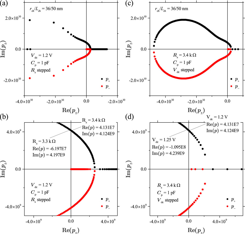
To understand the effects of parameters $R_{\text{s}}$, $C_{\text{p}}$, and $V_{\text{dc}}$ on the dynamical behavior of a Mott memristor PA oscillator, we first calculated the values of the pair of poles $p_{\pm }$ of its small-signal transfer function $H(s;Q)$, using Equation 53 by varying one parameter while keeping the other two parameters fixed. We then applied the parametric Nyquist plot technique to gain insights into the stability of the second-order system.

Let us first examine the effect of varying $R_{\text{s}}$ while keeping $C_{\text{p}}$ and $V_{\text{dc}}$ fixed. Figure 21A shows the Nyquist plot of Im$(p_{\pm })$ vs Re$(p_{\pm })$ for the midsize ${\text{VO}}_2$ Mott memristor PA oscillator with $C_{\text{p}}=1$ pF, $V_{\text{dc}}=1.2$ V, and $R_{\text{s}}$ stepped from 100 $\mathrm{\Omega }$ to 27 k$\mathrm{\Omega }$ at a 100 $\mathrm{\Omega }$ interval. It reveals three distinctive regions as $R_{\text{s}}$ increases: (1) when $R_{\text{s}}=100\mathrm{\Omega }-200\mathrm{\Omega }$, $p_{+}$ and $p_{-}$ are negative real numbers. (2) When $R_{\text{s}}=300\mathrm{\Omega }-7.5\text{\hspace{0.17em}k}\mathrm{\Omega }$, $p_{+}$ and $p_{-}$ form a complex conjugate pair. (3) When $R_{\text{s}}=7.6\text{\hspace{0.17em}k}\mathrm{\Omega }-27\text{\hspace{0.17em}k}\mathrm{\Omega }$, $p_{+}$ and $p_{-}$ are positive real numbers. Figure 21B presents a zoomed-in view of Figure 19A, which reveals that increasing $R_{\text{s}}$ from 3.3 k$\mathrm{\Omega }$ to 3.4 k$\mathrm{\Omega }$ flips the sign of Re$(p_{\pm })$ from negative to positive, i.e., the pair of poles crosses over from the LHP to the RHP. If we consider the second-order system an uncoupled one-port element and apply the first criterion of Chua’s LA theorem the element is locally active and unstable (LA$\backslash$EOC) at $R_{\text{s}}\ge 3.4$ k$\mathrm{\Omega }$ since $H(s;Q)$ has a pair of poles in the open RHP. At $R_{\text{s}}\le 3.3$ k$\mathrm{\Omega }$, both poles lie in the LHP, implying a local asymptotic stability. Since both the EOC and LP regions are locally stable, we need to use the fourth LA criterion (LA if $\text{Re}[H(i\omega ;Q)]<0$ for some finite $\omega$) to examine the system’s activity. It shows that the system is in the EOC region for $1135.4\mathrm{\Omega }\le R_{\text{s}}\le 3.3$ k$\mathrm{\Omega }$. At $R_{\text{s}}<1135.4\mathrm{\Omega }$, the system is LP. The second-order system’s EOC-LP crossover occurs when the oscillator’s load line $V=V_{\text{dc}}-I{R}_{\text{s}}$ intersects the steady-state locus of the memristor $M$ at the critical point $Q_0=(i_0,v_0)$ between the NDR and upper PDR regions (see Figure 14F). For the midsize VO₂ memristor, $i_0=971.18\mathrm{\mu }$A and $v_0=0.0973$ V. Note that this crossover coincides with the EOC-LP crossover for an isolated memristor $M$ (see Section 4.2.3). Extracting $\text{Re}[H(i\omega ;Q)]$ from Formula 47, one can derive the frequency limit for the EOC region as $f_{\text{max}}=\frac{1}{2\pi }\sqrt{\frac{-(R_{\text{s}}zp+R_2{z}^2)}{R_{\text{s}}+R_2}}$. At a fixed $V_{\text{dc}}$, $f_{\text{max}}$ grows with $R_{\text{s}}$ in a sublinear fashion. For the case of $V_{\text{dc}}=1.2$ V, $f_{\text{max}}$ rises from 182.5 MHz at $R_{\text{s}}=1.2$ k$\mathrm{\Omega }$ to 653.7 MHz at $R_{\text{s}}=3.3$ k$\mathrm{\Omega }$.

Figure 21

Figure 21. (A) Nyquist plot of Im$(p_{\pm })$ vs Re$(p_{\pm })$ for the pair of poles $p_{\pm }$ of the small-signal transfer function $H(s;Q)$ of the midsize ${\text{VO}}_2$ Mott memristor PA oscillator with $C_{\text{p}}=1$ pF, $V_{\text{dc}}=1.2$ V, and $R_{\text{s}}$ stepped from 100 $\mathrm{\Omega }$ to 27 k$\mathrm{\Omega }$ at a 100-$\mathrm{\Omega }$ interval. (B) Zoomed-in view of (A), showing that increasing $R_{\text{s}}$ from 3.3 k$\mathrm{\Omega }$ to 3.4 k$\mathrm{\Omega }$ turns Re$(p_{\pm })$ from negative to positive. (C) Nyquist plot of the same PA oscillator with $R_{\text{s}}=3.4\text{\hspace{0.17em}k}\mathrm{\Omega }$, $C_{\text{p}}=1$ pF, and $V_{\text{dc}}$ stepped from 0.55 V to 13.5 V at a 50-mV interval. (D) Zoomed-in view of (C), showing that increasing $V_{\text{dc}}$ from 1.2 V to 1.25 V turns Re$(p_{\pm })$ from positive to negative.

A similar crossover is observed by varying $V_{\text{dc}}$ while keeping $R_{\text{s}}$ and $C_{\text{p}}$ fixed. Figure 21C shows the Nyquist plot of Im$(p_{\pm })$ vs Re$(p_{\pm })$ for the midsize ${\text{VO}}_2$ Mott memristor PA oscillator with $R_{\text{s}}=3.4\text{\hspace{0.17em}k}\mathrm{\Omega }$, $C_{\text{p}}=1$ pF, and $V_{\text{dc}}$ stepped from 0.55 V to 13.5 V at 50-mV interval. It reveals the following two distinctive regions as $V_{\text{dc}}$ increases: (1) when $V_{\text{dc}}=0.55\text{\hspace{0.17em}V}-0.65\text{\hspace{0.17em}V}$, $p_{+}$ and $p_{-}$ are positive real numbers. (2) When $V_{\text{dc}}=0.7\text{\hspace{0.17em}V}-13.5\text{\hspace{0.17em}V}$, $p_{+}$ and $p_{-}$ form a complex conjugate pair. Figure 21D shows a zoomed-in view of Figure 21C, which reveals that increasing $V_{\text{dc}}$ from 1.2 V to 1.25 V flips the sign of Re$(p_{\pm })$ from positive to negative, i.e., the pair of poles crosses over from the RHP to the LHP. Applying the first LA criterion in a similar manner, the system is LA$\backslash$EOC at $V_{\text{dc}}\le 1.2$ V since $H(s;Q)$ has a pair of poles in the open RHP. At $V_{\text{dc}}\ge 1.25$ V, the system is locally stable since both poles lie in the LHP. The fourth LA criterion can be used to determine the system’s activity. It shows that the system is in the EOC region at 1.25 V $\le V_{\text{dc}}\le 3.3993$ V. At $V_{\text{dc}}>3.3993$ V, the system is LP. Once again, the system’s EOC-LP crossover occurs when the load line interects the steady-state locus of $M$ at $Q_0$. At a fixed $R_{\text{s}}$, the frequency limit $f_{\text{max}}$ for the EOC region decreases with $V_{\text{dc}}$ in a nonlinear fashion. For the case of $R_{\text{s}}=3.4$ k$\mathrm{\Omega }$, $f_{\text{max}}$ drops from 649.6 MHz at $V_{\text{dc}}=1.25$ V to 100.7 MHz at $V_{\text{dc}}=3.35$ V.

Instead of using the sign of Re$(p_{\pm })$ in the Cartesian coordinate as a test for the first LA criterion, one can also use the argument (phase) of a pole in the polar coordinate. The $p_{+}$ pole is located in the first and second quadrants, including the Re and Im + axes. Its complex conjugate $p_{-}$ is located in the third and fourth quadrants, including the Re and Im$-$ axes. We only need to examine arg$(p_{+})$, argument of the $p_{+}$ pole of $H(s;Q)$, as a test for the first LA criterion. A crossover from LA\EOC to EOC occurs if arg$(p_{+})$ increases from below $90°$ to above $90°$, i.e., $p_{+}$ moves from the first quadrant to the second quadrant by crossing the Im + axis.

At a fixed $C_{\text{p}}$ parameter, one can thus visualize the LA and LP operating regions of a Mott memristor PA oscillator by plotting a 2D color-scale map of arg$(p_{+})$ with $R_{\text{s}}$ and $V_{\text{dc}}$ parameters as the $x$ and $y$ coordinates, respectively. The $\text{arg}(p_{+})=90^{◦}$ contour line separates the EOC and LA$\backslash$EOC regions. Then the critical points from the load line analysis $V_{\text{dc}}=v_0+i_0{R}_{\text{s}}$ is superimposed to the color-scale map as the border line between the LP and EOC regions. Now, this 2D map can be referred to as a phase diagram for complexity for the second-order system. The procedure is then repeated at different $C_{\text{p}}$ values to observe how the LA and LP regions evolve as $C_{\text{p}}$ is adjusted. Figure 22 shows four 2D color-scale maps of arg$(p_{+})$ for the midsize ${\text{VO}}_2$ Mott memristor PA oscillator at $C_{\text{p}}=0.1$ pF (a), 1 pF (b), 10 pF (c), and 100 pF (d), respectively.

Figure 22

Figure 22. 2D color-scale maps of $\text{arg}(p_{+})(R_{\text{s}},V_{\text{dc}})$, argument of the $p_{+}$ pole of $H(s;Q)$, with $R_{\text{s}}$ and $V_{\text{dc}}$ as the $x$ and $y$ coordinates, respectively, for the midsize ${\text{VO}}_2$ Mott memristor PA oscillator at (A) $C_{\text{p}}=0.1$ pF, (B) $C_{\text{p}}=1$ pF, (C) $C_{\text{p}}=10$ pF, and (D) $C_{\text{p}}=100$ pF, respectively. In each plot, the LA\EOC region $(\text{Re}(p_{+})>0)$ and the EOC region $(\text{Re}(p_{+})<0$ and meets the fourth LA criterion) are separated by the $90°$ contour line (solid black line marked by “+“). The LP region $(\text{Re}(p_{+})<0$ and fails the fourth LA criterion) and the EOC region are separated by the straight line V_dc = v₀ + i₀R_s derived from the load line analysis (dashed white line). Here i₀ = 971.18 μA and v₀ = 0.0973 V. We use a cyclic color map with four distinct colors to allow four orientations or phase angles to be visualized. Both $\text{arg}(p_{+})=0°$ and $\text{arg}(p_{+})=180°$ are shown with the same color (pink).

We consider Figure 22A as an example to discuss their common characteristics. From the complex domain aspect, arg$(p_{+})$ has three distinctive regions if one navigates along the top right to bottom left diagonal. At small $V_{\text{dc}}$ and large $R_{\text{s}}$ (the top-right pink region), $\text{arg}(p_{+})=0°$ and $p_{+}$ is a positive real number on the Re + axis. At larger $V_{\text{dc}}$ and smaller $R_{\text{s}}$, $p_{+}$ is a complex number (the middle colored region) in either the first quadrant (LA\EOC) or the second quadrant (EOC), divided by the $90°$ contour line. At even larger $V_{\text{dc}}$ and smaller $R_{\text{s}}$, $\text{arg}(p_{+})=180°$ and $p_{+}$ is a negative real number on the Re$-$ axis. A notable feature is that all the borderlines between adjacent regions are straight lines that extend from the top left to the bottom right. Despite their appearance, they do not intersect at a common point if extrapolated toward the top-left direction. Note that the borderline separating the LP and EOC regions (dashed white line) does not vary with C_p.

The effect of $C_{\text{p}}$ can be observed by comparing the four color-scale maps. As $C_{\text{p}}$ increases from 0.1 pF to 10 pF, the arg(p+) = 90° borderline rotates clockwise, and the rotation stalls as $C_{\text{p}}$ further increases to 100 pF. The $\text{arg}(p_{+})=0°$ (positive real) region at the top right corner continuously expands with an increase in $C_{\text{p}}$, while the complex region shrinks with an increase in $C_{\text{p}}$. The $\text{arg}(p_{+})=180°$ (negative real) region at the bottom left corner initially shrinks significantly as $C_{\text{p}}$ increases from 0.1 pF to 1 pF, and then, it recovers a little as $C_{\text{p}}$ further increases. The size of LP region remains unchanged as C_p increases, while the size of EOC region gets compressed. At C_p = 100 pF, the EOC region barely exists as the two borderlines almost merge.

Using the element combination approach, we have shown that when a Mott memristor is coupled to a capacitor, both the system’s dimension and its dynamical complexity increases — a new LA\EOC region emerges to host instabilities and persistent oscillations. One can also examine the case of an inductively coupled Mott memristor, e.g., connecting an external inductor in parallel with a Mott memristor. It is found that the poles of the transfer function of such a composite circuit remain in the LHP; thus, the composite circuit does not satisfy the LA criterion to exhibit instabilities or persistent oscillations (Brown et al., 2022b). This is not surprising since an isolated Mott memristor has an inherently inductive reactance.

5.3 Jacobian matrix method

For second or higher-order nonlinear systems, the Jacobian matrix method is a linearization technique that allows local stability analysis near a hyperbolic fixed point. As an introduction in a nutshell, consider an autonomous system of ODEs $\dot{\mathbf{x}}=\mathbf{f}(\mathbf{x})$, where $\dot{\mathbf{x}}$ is the component-wise time derivative for the set of state variables x. x corresponds to a point in an open subset of real $n$-space, $E\subset {\mathbb{R}}^n$. $\mathbf{f}:E\to {\mathbb{R}}^n$ is a differentiable function that describes the dynamics of x. f is also called a vector field since the mapping from x to f(x) assigns a vector. For a 2D (planar) system described by $\frac{dx}{dt}=f(x,y)$ and $\frac{dy}{dt}=g(x,y)$, $\mathbf{f}(\mathbf{x})=(f(x,y),g(x,y))$ can be visualized using a vector based at the point $(x,y)$, whose $x$- and $y$-components are $f(x,y)$ and $g(x,y)$, respectively. The set of solutions $\varphi (t,{\mathbf{x}}_0)$ of the initial value problem $\dot{\mathbf{x}}=\mathbf{f}(\mathbf{x})$, with $\mathbf{x}(0)={\mathbf{x}}_0\in E$, is called the flow of the ODE or the flow of the vector field f. For each initial condition ${\mathbf{x}}_0$, $\varphi (t,{\mathbf{x}}_0)$ provides the trajectory of a unique solution of the ODE, which is called the orbit of x under $\varphi$.

In autonomous systems, f does not explicitly depend on time. If $\mathbf{f}({\mathbf{x}}_Q)=0$, i.e., its time derivative is 0, then ${\mathbf{x}}_Q$ is a fixed point. The Jacobian matrix Df, or simply Jacobian, is the matrix of all the first-order partial derivatives of f(x). The Hartman–Grobman theorem and the stable manifold theorem guarantee that the local qualitative behavior of a nonlinear system $\dot{\mathbf{x}}=\mathbf{f}(\mathbf{x})$ near a hyperbolic fixed point ${\mathbf{x}}_Q$ is determined by a linear system $\dot{\mathbf{x}}=A\mathbf{x}$, where $A=D\mathbf{f}({\mathbf{x}}_Q)$ is the Jacobian of f at ${\mathbf{x}}_Q$. In other words, the flow of a nonlinear system is topologically conjugate to that of its linearized system in some neighborhood of a fixed point, provided the fixed point is hyperbolic. If the Jacobian is a square matrix and none of the eigenvalues of $D\mathbf{f}({\mathbf{x}}_Q)$ is a pure imaginary number, then the fixed point is hyperbolic, and its stability can be told by the signs of the real parts of the eigenvalues, as will be elaborated later.

Next, we consider the Jacobian matrix approach to analyze the local stability of a Mott memristor PA oscillator. This second-order system is described by Equations 55–57.

$v=R_{\text{ch}}\left(x\right)i_{\text{M}},(55)$

$\frac{dx}{dt}=f_x\left(x,i_{\text{M}}\right),(56)$

$\frac{dv}{dt}=\frac{1}{C_{\text{p}}}\left(\frac{V_{\text{dc}}-v}{R_{\text{s}}}-i_{\text{M}}\right),(57)$

where $f_x(x,i_{\text{M}})$ and $R_{\text{ch}}(x)$ are the kinetic and memristance functions of the memristor $M$, respectively. $i_{\text{M}}$ is the current flowing through $M$. Substituting it with $v/R_{\text{ch}}(x)$, we obtain the two coupled ODEs (Equations 58, 59) that describe the system dynamics.

$\frac{dx}{dt}\triangleq f\left(x,v\right)=f_x\left(x,\frac{v}{R_{\text{ch}}\left(x\right)}\right),(58)$

$\frac{dv}{dt}\triangleq g\left(x,v\right)=\frac{1}{C_{\text{p}}}\left(\frac{V_{\text{dc}}-v}{R_{\text{s}}}-\frac{v}{R_{\text{ch}}\left(x\right)}\right).(59)$

In a vector form, the system is described as $\dot{\mathbf{x}}=\mathbf{f}(\mathbf{x})$. Here, $\dot{\mathbf{x}}={[x,v]}^{\text{T}}$ is the state variable vector, and $\mathbf{f}(\mathbf{x})={[f(x,v),g(x,v)]}^{\text{T}}$ is the differentiable function that describes the dynamics of x. Around a fixed point $Q$ with a coordinate $(x_Q,v_Q)$, the Jacobian matrix Df of the system is a 2 × 2 matrix of all the first-order partial derivatives of f(x) that takes the following form:

${\left.D\mathbf{f}\right|}_Q=\left[\begin{array}{cc}\hfill {\xi }_{11}\hfill & \hfill {\xi }_{12}\hfill \\ \hfill {\xi }_{21}\hfill & \hfill {\xi }_{22}\hfill \end{array}\right]=\left[\begin{array}{cc}\hfill {\left.\frac{\partial f\left(x,v\right)}{\partial x}\right|}_Q\hfill & \hfill {\left.\frac{\partial f\left(x,v\right)}{\partial v}\right|}_Q\hfill \\ \hfill {\left.\frac{\partial g\left(x,v\right)}{\partial x}\right|}_Q\hfill & \hfill {\left.\frac{\partial g\left(x,v\right)}{\partial v}\right|}_Q\hfill \end{array}\right].(60)$

The four elements of the Jacobian matrix are derived as follows:

${\xi }_{11}={\left.\frac{\partial f\left(x,v\right)}{\partial x}\right|}_Q=b_{11}\left(Q\right)-\frac{b_{12}\left(Q\right)a_{11}\left(Q\right)}{R_{\text{ch}}\left(x_Q\right)},(61)$

${\xi }_{12}={\left.\frac{\partial f\left(x,v\right)}{\partial v}\right|}_Q=\frac{b_{12}\left(Q\right)}{R_{\text{ch}}\left(x_Q\right)},(62)$

${\xi }_{21}={\left.\frac{\partial g\left(x,v\right)}{\partial x}\right|}_Q=\frac{a_{11}\left(Q\right)}{R_{\text{ch}}\left(x_Q\right)C_{\text{p}}},(63)$

${\xi }_{22}={\left.\frac{\partial g\left(x,v\right)}{\partial v}\right|}_Q=-\left(\frac{1}{R_{\text{s}}{C}_{\text{p}}}+\frac{1}{R_{\text{ch}}\left(x_Q\right)C_{\text{p}}}\right).(64)$

The eigenvalues of the Jacobian around a fixed point $Q$ derived through Equations 60–64 are calculated by solving its characteristic equation that can be expanded to a quadratic polynomial.

$\begin{array}{ll}\hfill \left(D\mathbf{f}-\lambda I\right){|}_Q& ={\lambda }^2-\mathrm{t}\mathrm{r}\left(D\mathbf{f}\right)\lambda +\mathrm{d}\mathrm{e}\mathrm{t}\left(D\mathbf{f}\right)\hfill \\ \hfill & ={\lambda }^2-\left({\xi }_{11}+{\xi }_{22}\right)\lambda +\left({\xi }_{11}{\xi }_{22}-{\xi }_{12}{\xi }_{21}\right),\hfill \end{array}(65)$

where $I$ is the identity matrix. $\mathrm{t}\mathrm{r}(D\mathbf{f})$ is the trace of the Jacobian matrix, and $\mathrm{d}\mathrm{e}\mathrm{t}(D\mathbf{f})$ is its determinant. For simplicity, we use $\mathrm{t}\mathrm{r}$ and $\mathrm{d}\mathrm{e}\mathrm{t}$ to represent them hereafter. Their expressions are derived as follows:

$\mathrm{t}\mathrm{r}=-\left[{\omega }_1\left(1+\frac{R_1}{R_{\text{ch}}}\right)+{\omega }_0\left(1+\frac{R_{\text{s}}}{R_{\text{ch}}}\right)\right],(66)$

$\mathrm{d}\mathrm{e}\mathrm{t}={\omega }_1{\omega }_0\left(1+\frac{R_1}{R_{\text{ch}}}+\frac{R_{\text{s}}}{R_{\text{ch}}}\right),(67)$

where we define another cutoff frequency ${\omega }_1\triangleq {(R_1{C}_1)}^{-1}$, in addition to the previously defined cutoff frequency ${\omega }_0={(R_{\text{s}}{C}_{\text{p}})}^{-1}$, to simplify the expressions.

The two roots ${\lambda }_{+}$ and ${\lambda }_{-}$ of the characteristic equation (Equation 65) are

${\lambda }_{\pm }=\frac{\mathrm{t}\mathrm{r}\pm \sqrt{{\mathrm{t}\mathrm{r}}^2-4\mathrm{d}\mathrm{e}\mathrm{t}}}{2}.(68)$

Note that ${\lambda }_{+}+{\lambda }_{-}=\mathrm{t}\mathrm{r}$ and ${\lambda }_{+}{\lambda }_{-}=\mathrm{d}\mathrm{e}\mathrm{t}$, i.e., trace is the sum of eigenvalues, and determinant is the product of them. The discriminant ${\mathrm{t}\mathrm{r}}^2-4\mathrm{d}\mathrm{e}\mathrm{t}$ of the characteristic equation in the expanded form is

$\begin{array}{l}\hfill {\mathrm{t}\mathrm{r}}^2-4\mathrm{d}\mathrm{e}\mathrm{t}={\omega }_1^2{\left(1+{\gamma }_1\right)}^2+{\omega }_0^2{\left(1+{\gamma }_{\text{s}}\right)}^2-2{\omega }_1{\omega }_0\left[\left(1-{\gamma }_1\right){\gamma }_{\text{s}}+\left(1+{\gamma }_1\right)\right],\end{array}(69)$

where we define two dimensionless resistance ratios ${\gamma }_1\triangleq \frac{R_1}{R_{\text{ch}}}$ and ${\gamma }_{\text{s}}\triangleq \frac{R_{\text{s}}}{R_{\text{ch}}}$ to simplify the expression.

5.4 Trace–determinant plane classification

For a 2D homogeneous linear system $\dot{\mathbf{x}}=A\mathbf{x}$, the parameter space of a trace–determinant (tr–det) plane allows the qualitative classification of its fixed points. In this study, a homogeneous linear system is defined in contrast to a nonhomogeneous linear system $\dot{\mathbf{x}}=A\mathbf{x}+\mathbf{h}(t)$, which includes a vector of functions $\mathbf{h}(t)$ that are independent of solutions and their derivatives. For a 2D nonlinear system, after linearization, one needs to be cautious when applying the tr–det plane method since linearization may change the nature of its fixed points, especially along the borderlines on the tr–det plane. Here, we examine the tr–det plane method on a linearized Mott memristor PA oscillator to check whether one can gain some insights into the original nonlinear system.

In a tr–det plane, a coordinate (tr, det) corresponds to a Jacobian matrix with trace tr and determinant det. The location of this point relative to the parabola curve ${\mathrm{t}\mathrm{r}}^2-4\mathrm{d}\mathrm{e}\mathrm{t}=0$ determines the geometry of the phase portrait. The sign of the discriminant ${\mathrm{t}\mathrm{r}}^2-4\mathrm{d}\mathrm{e}\mathrm{t}$ in Equation 69 divides the eigenvalues of $D\mathbf{f}$ into the following regions.

a) If ${\mathrm{t}\mathrm{r}}^2-4\mathrm{d}\mathrm{e}\mathrm{t}>0$, ${\lambda }_{+}$ and ${\lambda }_{-}$ are real and distinct.

b) If ${\mathrm{t}\mathrm{r}}^2-4\mathrm{d}\mathrm{e}\mathrm{t}<0$, ${\lambda }_{+}$ and ${\lambda }_{-}$ are complex conjugates with a nonzero imaginary part.

c) If ${\mathrm{t}\mathrm{r}}^2-4\mathrm{d}\mathrm{e}\mathrm{t}=0$, ${\lambda }_{+}$ and ${\lambda }_{-}$ are real and repeated (identical).

Within each of these three regions, the tr–det plane further classifies the dynamics and stability of isolated or non-isolated fixed points as enumerated below. The numbers within () that appear out of order are class identifiers (IDs), provided in Table 3, which is a tabulated summary of the tr–det plane classification. It is notable that the only stable region in the tr–det plane is the closed second quadrant, i.e., $\mathrm{t}\mathrm{r}\le 0$ and $\mathrm{d}\mathrm{e}\mathrm{t}\ge 0$. If a fixed point is stable, its eigenvalues ${\lambda }_{+}$ and ${\lambda }_{-}$ must both be negative real: $({\lambda }_{+},{\lambda }_{-})\le 0$ or they are complex conjugates with a negative real part: $\mathrm{R}\mathrm{e}({\lambda }_{+},{\lambda }_{-})\le 0$.

Table 3

Table 3. Trace–determinant (tr–det) plane classification of fixed points for 2D linear homogeneous systems. In the tr–det plane, the only stable region is the closed second quadrant, i.e., $\mathrm{t}\mathrm{r}\le 0$ and $\text{det}\ge 0$.

Region (a) with two real and distinct eigenvalues ${\lambda }_{+}\ne {\lambda }_{-}$

(1) ${\lambda }_{+}>0>{\lambda }_{-}$: unstable saddle point

(2) ${\lambda }_{+}=0,{\lambda }_{-}<0$: stable line of non-isolated fixed points

(4) ${\lambda }_{+}>0,{\lambda }_{-}=0$: unstable line of non-isolated fixed points

(5) $0>{\lambda }_{+}>{\lambda }_{-}$: stable sink

(13) ${\lambda }_{+}>{\lambda }_{-}>0$: unstable source

Region (b) with a pair of complex conjugate eigenvalues ${\lambda }_{\pm }=\alpha \pm \beta i$, $\beta \ne 0$

(8) $\mathrm{R}\mathrm{e}({\lambda }_{\pm })<0$: stable spiral sink

(9) $\mathrm{R}\mathrm{e}({\lambda }_{\pm })=0$: stable center (not asymptotically stable)

(10) $\mathrm{R}\mathrm{e}({\lambda }_{\pm })>0$: unstable spiral source

A center is a non-hyperbolic fixed point since it has a pair of pure imaginary eigenvalues; therefore, the Hartman–Grobman theorem is not applicable. It is stable (or Lyapunov stable) but not asymptotically stable. A solution that starts near a center remains close to it but never converges over time since non-zero pure imaginary eigenvalues correspond to periodic solutions that oscillate without damping.

Region (c) with real and repeated eigenvalues: ${\lambda }_{\pm }=\lambda$

(3) $\lambda =0$: parallel lines of non-isolated fixed points or the entire plane

(6) $\lambda <0$ and is incomplete: stable degenerate sink

(7) $\lambda <0$ and is complete: stable star sink

(11) $\lambda >0$ and is incomplete: unstable degenerate source

(12) $\lambda >0$ and is complete: unstable star source

Here, a nonzero real and repeated eigenvalue is considered complete if it has two linearly independent eigenvectors, making the fixed point (star) a proper node. Otherwise, if the eigenvalue is incomplete (has only one eigenvector), the fixed point is classified as a degenerate or improper node.

For a linearized 2D nonlinear system, the tr-det plane predictions are always accurate for classes 1, 5, 8, 10, and 13. While predictions for the other eight classes may not be accurate, they correctly determine the stability of classes 6, 7, 11, and 12. Prediction for class 9 is accurate if the system is conservative.

Now, we apply the tr–det plane analysis for the 2D nonlinear system of the ${\text{VO}}_2$Mott memristor PA oscillator. This system has been analyzed previously using an element combination approach by considering a Mott memristor $M$and a capacitor $C_{\text{p}}$in parallel as a composite second-order nonlinear element $Z_{\text{CM}}$, which is connected to a resistor $R_{\text{s}}$in series. The small-signal transfer function of this 2D nonlinear system has two poles $p_{\pm }$that form a pair of complex conjugate in part of the circuit parameter space. The Nyquist plots in Figures 21A, Bshow the evolution of the positions of $p_{\pm }$as $R_{\text{s}}$is varied while keeping $C_{\text{p}}=1$pF and $V_{\text{dc}}=1.2$V unchanged. Increasing $R_{\text{s}}$from 3.3 k$\mathrm{\Omega }$to 3.4 k$\mathrm{\Omega }$flips the sign of Re$(p_{\pm })$from negative to positive and produces a crossover from EOC to LA\EOC as per Chua’s LA theorem.

Instead of element combination, we now apply the tr–det plane analysis of the Jacobian linearized 2D PA oscillator system. We show that the 2D tr–det plane method elucidates the nature of this crossover in local activity to be a bifurcation, which changes the stability of an isolated fixed point. Figure 23A plots the (tr, det) plane that is geometrically divided into different regions by the tr- and det-axes and the $\mathrm{d}\mathrm{e}\mathrm{t}={\mathrm{t}\mathrm{r}}^2/4$ parabola. Each of them is labeled by the class IDs, as listed in Table 3. It shows a locus of (tr, det) calculated from the Jacobian matrix of the midsize ${\text{VO}}_2$ Mott memristor PA oscillator around its fixed points by fixing $C_{\text{p}}=1$ pF, $V_{\text{dc}}=1.2$ V, and stepping $R_{\text{s}}$ from 100 $\mathrm{\Omega }$ to 17.2 k$\mathrm{\Omega }$ at 100 $\mathrm{\Omega }$ interval. The (tr, det) points for $100\mathrm{\Omega }\le R_{\text{s}}\le 600\mathrm{\Omega }$ outside the plotted area are all located above the $\mathrm{d}\mathrm{e}\mathrm{t}={\mathrm{t}\mathrm{r}}^2/4$ parabola within the same stable spiral sink (class 8) region. The trajectory of (tr, det) formed by varying $R_{\text{s}}$ is nonlinear and convex-shaped. Increasing $R_{\text{s}}$ moves (tr, det) toward the region of an unstable spiral source (class 10) in the first quadrant and produces a bifurcation as it crosses the positive $\mathrm{d}\mathrm{e}\mathrm{t}$ axis. At $R_{\text{s}}>7.5$ k$\mathrm{\Omega }$, (tr, det) of the fixed point crosses the $\mathrm{d}\mathrm{e}\mathrm{t}={\mathrm{t}\mathrm{r}}^2/4$ parabola into the unstable source (class 13) region, but its stability remains unchanged. Therefore, $R_{\text{s}}$ is clearly a bifurcation parameter for the 2D PA oscillator.

Figure 23

Figure 23. (A) Trace–determinant plane showing the (tr, det) locus for the Jacobian of the midsize ${\text{VO}}_2$ Mott memristor PA oscillator with $C_{\text{p}}=1$ pF, $V_{\text{dc}}=1.2$ V, and bifurcation parameter $R_{\text{s}}$ stepped from 100 $\mathrm{\Omega }$ to 17.2 k$\mathrm{\Omega }$ at a 100-$\mathrm{\Omega }$ interval. (B) Zoomed-in view of (A), showing that increasing $R_{\text{s}}$ from 3.3 k$\mathrm{\Omega }$ to 3.4 k$\mathrm{\Omega }$ results in a bifurcation from a stable spiral sink (class 8) to an unstable spiral source (class 10). At ${R*}_{\text{s}}=3359.5$ $\mathrm{\Omega }$, the fixed point is a stable center (class 9) located on the $\mathrm{t}\mathrm{r}=0$ axis. (C) The (tr, det) locus for the Jacobian of the same PA oscillator, with $R_{\text{s}}=3.4\text{\hspace{0.17em}k}\mathrm{\Omega }$, $C_{\text{p}}=1$ pF, and bifurcation parameter $V_{\text{dc}}$ stepped from 1 V to 3 V at a 10-mV interval. (D) Zoomed-in view of (C), showing that increasing $V_{\text{dc}}$ from 1.21 V to 1.22 V produces a bifurcation from an unstable spiral source (class 10) to a stable spiral sink (class 8). At ${V*}_{\text{dc}}=1.21355$ V, the fixed point is a stable center (class 9) located on the positive $\mathrm{d}\mathrm{e}\mathrm{t}$ axis.

Figure 23B is a zoomed-in view of (a). It shows that increasing $R_{\text{s}}$ from 3.3 k$\mathrm{\Omega }$ to 3.4 k$\mathrm{\Omega }$ produces a stability-change bifurcation from a stable spiral sink (class 8) to an unstable spiral source (class 10), both belonging to Region (b) of ${\mathrm{t}\mathrm{r}}^2-4\mathrm{d}\mathrm{e}\mathrm{t}<0$ that has complex conjugate Jacobian eigenvalues. At a critical value of ${R*}_{\text{s}}=3359.5$ $\mathrm{\Omega }$, (tr, det) is located exactly on the $\mathrm{t}\mathrm{r}=0$ axis as the borderline between the unstable first quadrant and stable second quadrant. The tr–det plane predicts that the fixed point is a stable center (class 9). We have learned that predictions about a spiral sink (class 8) and a spiral source (class 10) are always correct for 2D nonlinear systems, but the prediction about a center (class 9) is unproven since a 2D PA oscillator is not a conservative system.

In Figure 23C, we plot the (tr, det) locus for the Jacobian of the same PA oscillator around its fixed points, this time by fixing $R_{\text{s}}=3.4\text{\hspace{0.17em}k}\mathrm{\Omega }$, $C_{\text{p}}=1$ pF, and stepping $V_{\text{dc}}$ from 1 V to 3 V at a 10-mV interval. It shows a similarly shaped convex trajectory of (tr, det) as the case for stepping $R_{\text{s}}$. However, the effect of $V_{\text{dc}}$ is opposite to that of $R_{\text{s}}$ a larger $V_{\text{dc}}$ moves (tr, det) toward the stable spiral sink (class 8) region in the second quadrant. Figure 23D is a zoomed-in view of (c), showing that increasing $V_{\text{dc}}$ from 1.21 V to 1.22 V produces a stability-change bifurcation from an unstable spiral source (class 10) to a stable spiral sink (class 8). At a critical value of ${V*}_{\text{dc}}=1.21355$ V, (tr, det) is located exactly on the $\mathrm{t}\mathrm{r}=0$ axis. Therefore, $V_{\text{dc}}$ is also a bifurcation parameter for the 2D PA oscillator. The fact that the critical values of bifurcation parameters $R_{\text{s}}$ and $V_{\text{dc}}$, as determined by the tr-det plane analysis, closely match with those obtained from the small-signal Nyquist plot analysis using the element combination approach (see Figure 21) corroborates the validity of both methods.

The parallel capacitor $C_{\text{p}}$ also functions as a bifurcation parameter if $R_{\text{s}}$ and $V_{\text{dc}}$ are fixed and $C_{\text{p}}$ is adjusted. Figure 24A shows the plots of four loci of the Jacobian (tr, det) for the midsize ${\text{VO}}_2$ Mott memristor PA oscillator, with $V_{\text{dc}}=1.2$ V and $R_{\text{s}}$ fixed at 3 k$\mathrm{\Omega }$, 5 k$\mathrm{\Omega }$, 7 k$\mathrm{\Omega }$, and 9 k$\mathrm{\Omega }$, respectively. For each locus, we step up $C_{\text{p}}$ in the sequence of 10 fF, 20 fF, 50 fF, 0.1 pF, 0.2 pF, 0.5 pF, 1 pF, 2 pF, 5 pF, and 10 pF. Similar to the case of varying $R_{\text{s}}$, increasing $C_{\text{p}}$ also moves (tr, det) from the stable second quadrant into the unstable first quadrant. However, the (tr, det) locus is linear instead of convex-shaped. Equations 66, 67 together predict a slope of $-{\omega }_1\left[1+R_1/\left(R_{\text{ch}}+R_{\text{s}}\right)\right]$ for the (tr, det) locus if $C_{\text{p}}$ is varied, which matches exactly with the linear regression slopes of the four loci. Equation 67 also predicts that (tr, det) asymptotically approaches the positive $\mathrm{t}\mathrm{r}$ axis as one continuously increases $C_{\text{p}}$ but never reaches it. Open symbols highlight the critical ${C*}_{\text{p}}$ values for the stability-change bifurcation as the (tr, det) loci intercept the positive $\mathrm{d}\mathrm{e}\mathrm{t}$ axis. It can be observed that a larger fixed $R_{\text{s}}$ would shift the (tr, det) locus upward and decrease its critical ${C*}_{\text{p}}$ value. Figure 24B shows the plots of the dependence of critical ${C*}_{\text{p}}$ on $R_{\text{s}}$ in a log–log fashion for three different $V_{\text{dc}}$ settings at 1.0 V, 1.2 V, and 1.4 V. One can infer that ${C*}_{\text{p}}(R_{\text{s}})$ follows a power law with an exponent close to $-2.5$. For the trace at $V_{\text{dc}}=1.2$ V, we added the point of $R_{\text{s}}=3359.5$ $\mathrm{\Omega }$. The power law predicts a ${C*}_{\text{p}}=1$ pF. which is consistent with the critical $({R*}_{\text{s}},C_{\text{p}})$ value for the same bifurcation in the case of varying $R_{\text{s}}$ at a fixed $C_{\text{p}}=1$ pF (see Figure 23B).

Figure 24

Figure 24. (A) Trace–determinant plane showing four (tr, det) loci for the Jacobian of the midsize ${\text{VO}}_2$ Mott memristor PA oscillator with $R_{\text{s}}=3$ k$\mathrm{\Omega }$, 5 k$\mathrm{\Omega }$, 7 k$\mathrm{\Omega }$, and 9 k$\mathrm{\Omega }$, respectively, all at $V_{\text{dc}}=1.2$ V. For each locus, increasing $C_{\text{p}}$ (from 10 fF to 10 pF in the present case) moves the Jacobian (tr, det) along a linear trajectory from the stable second quadrant into the unstable first quadrant, which then asymptotically approaches the positive $\mathrm{t}\mathrm{r}$ axis. The open symbol that intercepts the positive $\mathrm{d}\mathrm{e}\mathrm{t}$ axis shows the critical ${C*}_{\text{p}}$ for the source–sink bifurcation. (B) Log–log plot of the critical ${C*}_{\text{p}}$ vs $R_{\text{s}}$ for three cases of $V_{\text{dc}}=1.0$ V, 1.2 V and 1.4 V. Dashed lines are power-law fits ${C*}_{\text{p}}=a{R}_{\text{s}}^b$, with an exponent $b\approx -2.5$. The square (red) shows that ${C*}_{\text{p}}=1$ pF if $R_{\text{s}}=3359.5$ $\mathrm{\Omega }$, which is consistent that shown in Figure 23B.

6 Global analysis of reactively coupled Mott memristors: two-dimensional relaxation oscillator

6.1 Nullclines and direction field

The local analysis techniques we have discussed so far require a foreknowledge of the fixed points for a 2D nonlinear system. Global analyses, such as nullclines in the phase space of state variables, can be used to analyze a nonlinear system of ODEs and locate its fixed points. For a 2D or planar system, the $x$- (or $y$-) nullcline is defined as the set of points in the phase plane of $(x,y)$, where the time derivative of $x$ (or $y$) vanishes. Therefore, the vector field is vertical on the $x$-nullcline and horizontal on the $y$-nullcline. Together, they partition ${\mathbb{R}}^2$ into different open regions, each characterized by differences in the signs of their time derivatives. One can then determine the direction of the vector field in each region. The intersections of the $x$- and $y$-nullclines yield the fixed points. A direction field (also called a slope field) is the scaled version of a vector field, with all the vector lengths normalized to unity. In the 2D phase plane, superimposing the $x$- and $y$-nullclines onto the direction field reveals fixed points and provides insights into their dynamical classification and the orbits of solutions.

For the case of a 2D Mott memristor PA oscillator, the $x$-nullcline $(x_0,v_0)$ is the locus of points, where the time derivative of the state variable $x$ for the memristor $M$ vanishes

$f\left(x_0,v_0\right)=f_x\left(x_0,\frac{v_0}{R_{\text{ch}}\left(x_0\right)}\right)=0,(70)$

which can be rewritten as

$v_0={\left[-A\left(1+B{x}_0^2\right)\frac{\ln x_0}{C}\right]}^{-0.5}.(71)$

Since $(x_0,v_0)$ are steady states of $M$, the $x$-nullcline only depends on the internal characteristics of $M$ and is independent of the external circuit parameters including $R_{\text{s}}$, $C_{\text{p}}$, and $V_{\text{dc}}$. It remains the same as that of an isolated $M$ (see Figure 7C).

The $v$-nullcline $(x_1,v_1)$ is the locus of points where the time derivative of the state variable $v$ vanishes.

$g\left(x_1,v_1\right)=\frac{1}{C_{\text{p}}}\left(\frac{V_{\text{dc}}-v_1}{R_{\text{s}}}-\frac{v_1}{R_{\text{ch}}\left(x_1\right)}\right)=0,(72)$

which can be rewritten as

$v_1=\frac{V_{\text{dc}}}{1+R_{\text{s}}A\left(1+B{x}_1^2\right)}.(73)$

Since $v$ is the voltage across the capacitor $C_{\text{p}}$ and $M$ in parallel, the charge stored on the capacitor does not change over time; thus, there is no current flowing through it. Therefore, $R_{\text{s}}$ in series with $M$ forms a voltage divider. The $v$-nullcline depends on $V_{\text{dc}}$ and $R_{\text{s}}$, but it is independent of $C_{\text{p}}$.

The intersections of the $x$- and $y$-nullclines derived through Equations 70–73 are the fixed points $Q$ of the 2D system, where both $x$- and $v$-derivatives vanish.

$f\left(x_Q,v_Q\right)=f_x\left(x_Q,\frac{v_Q}{R_{\text{ch}}\left(x_Q\right)}\right)=0,(74)$

$g\left(x_Q,v_Q\right)=\frac{1}{C_{\text{p}}}\left(\frac{V_{\text{dc}}-v_Q}{R_{\text{s}}}-\frac{v_Q}{R_{\text{ch}}\left(x_Q\right)}\right)=0.(75)$

Figure 25 shows the plots of the $x$- and $v$-nullclines and direction field in the phase plane of the midsize ${\text{VO}}_2$ Mott memristor PA oscillator with $R_{\text{s}}=3.4$ k$\mathrm{\Omega }$ and $V_{\text{dc}}=1.2$ V. Note that the direction field depends on $C_{\text{p}}$ and is plotted for the case of $C_{\text{p}}=1.0$ pF. Under these conditions, the 2D nonlinear system has just one fixed point $(x_Q,v_Q)=(0.30396,0.12564)$ at the single intersection of the $x$-nullcline (blue-violet line) and $v$-nullcline (brown line) satisfying Equations 74, 75. The $x$- and $v$-nullclines partition the phase plane into four open regions, depending on the signs of time derivatives for $x$ and $v$, labeled as $(++)$, $(+-)$, $(-+)$, and $(--)$, respectively. The direction field (arrowheads) shows a distinct clockwise rotational pattern around $Q$, suggesting that the orbit of a solution $(x(t),v(t))$ with an initial condition close to $Q$ would rotate around it in a clockwise manner. Intuitively, if $Q$ were a stable spiral sink, $(x(t),v(t))$ would spiral inward toward it. If $Q$ were an unstable spiral source, $(x(t),v(t))$ would spiral outward. However, it is also possible that $(x(t),v(t))$ forms an isolated periodic orbit, continuously rotating around $Q$. Additional analyses are required in addition to the studies on the nullclines and direction field to determine whether such a case exists.

Figure 25

Figure 25. Nullclines and direction field (arrowheads) in the phase plane of the midsize ${\text{VO}}_2$ Mott memristor PA oscillator with $R_{\text{s}}=3.4$ k$\mathrm{\Omega }$, $C_{\text{p}}=1.0$ pF, and $V_{\text{dc}}=1.2$ V. Under these conditions, the 2D nonlinear system has one fixed point $(x_Q,v_Q)=(0.30396,0.12564)$ at the single intersection of the $x$- (blue-violet line) and $v$- (brown line) nullclines. Based on the signs of $dx/dt$ and $dv/dt$, the $x$- and $v$-nullclines partition the ${\mathbb{R}}^2$ plane into four open regions labeled as $(++)$, $(+-)$, $(-+)$, and $(--)$, respectively.

Since the location of the $v$-nullcline varies with $V_{\text{dc}}$ and $R_{\text{s}}$, decreasing $V_{\text{dc}}$ will shift it downward with respect to the $x$-nullcline, which may change the number of intersections between them. To investigate this, Figure 26 presents the three sets of $x$- and $v$-nullclines along the direction field for the same model PA oscillator at $V_{\text{dc}}$ values of 1.0379 V, 1.0 V and 0.519 V, respectively. Figure 26A and its zoomed-in view (Figure 26B) show the case of $V_{\text{dc}}=1.0379$ V. At this critical value of $V_{\text{dc}}$, the $v$-nullcline becomes tangent with the $x$-nullcline near its peak at the PDR-to-NDR crossover ${Q*}_a=(0.00589,1.00681)$, increasing the number of fixed points from one to two.

Figure 26

Figure 26. Nullclines and direction fields (arrowheads) in the phase plane of the midsize ${\text{VO}}_2$ Mott memristor PA oscillator with $R_{\text{s}}=3.4$ k$\mathrm{\Omega }$, $C_{\text{p}}=1.0$ pF, and $V_{\text{dc}}$ at (A) 1.0379 V, (C) 1.0 V, and (E) 0.519 V. (B), (D, F) Zoomed-in views to reveal semi-stable $(\times )$, stable $(•)$, and unstable $(◦)$ fixed points at the intersections of the $x$- (blue-violet line) and $v$- (brown line) nullclines.

Further reducing $V_{\text{dc}}$ will split ${Q*}_a$ into a pair of unstable $(Q_2)$ and stable $(Q_3)$ fixed points, which move apart from each other as $V_{\text{dc}}$ further decreases. This is a characteristic of a 2D saddle-node bifurcation. We are already familiar with the 1D case for an isolated Mott memristor (see Figure 6). To illustrate, Figure 26C and its zoomed-in view (Figure 26D) show the case of $V_{\text{dc}}=1.0$ V. Now, there are three intersections between the $v$- and $x$-nullclines. In addition to the original fixed point $Q_1=(0.25937,0.13823)$ located in the NDR region of $M$, two new fixed points $Q_2=(0.01064,0.96326)$ and $Q_3=(0.00243,0.97254)$ emerge at very small $x$ values. As a result, the ${\mathbb{R}}^2$ plane is now partitioned into six open regions instead of four. The two additional regions are $(++)$ within the PDR region of $M$ and $(--)$ near the PDR-to-NDR transition of $M$. The direction field reveals that $Q_2$ is an unstable node, while $Q_3$ is a stable node at an intersection in the PDR region (insulating state) of $M$.

$Q_1$ and $Q_2$ approach each other as $V_{\text{dc}}$ further decreases. Figure 26E and its zoomed-in view (Figure 26F) show that at another critical value of $V_{\text{dc}}=0.519$ V, the $v$-nullcline becomes tangent to the $x$-nullcline in its NDR region as $Q_1$ and $Q_2$ merge into one fixed point ${Q*}_b$. This fixed point disappears if $V_{\text{dc}}$ continues to decrease. At $V_{\text{dc}}<0.519$ V, only one stable fixed point $Q_3$ exists in the insulating state of $M$.

6.2 2D saddle-node bifurcations by varying V_dc

Plotting nullclines and direction fields at different values of $V_{\text{dc}}$ allowed us to identify two bifurcations, both appear to be 2D saddle-node bifurcations. Next, we apply the bifurcation diagram and tr–det plane methods to clarify their nature. We step the bifurcation parameter $V_{\text{dc}}$ from 3.0 V to 0 V at an interval of 0.01 V while keeping the other parameters unchanged and solve the fixed points $(x_Q,v_Q)$ by finding all the intersections of $x$- and $v$-nullclines. Figures 27A, B show the bifurcation diagrams for $x_Q$ and $v_Q$, respectively. Solid (open) circles are used for stable (unstable) fixed points. There exist three distinctive regions (I, II, and III) according to the number of fixed points at a specific $V_{\text{dc}}$. In region I ($V_{\text{dc}}>1.0379$ V), there is only one fixed point $Q_1$. The tr–det plane analysis (Figure 23D) reveals that $Q_1$ has a stability-change bifurcation at $V_{\text{dc}}=1.21355$ V (labeled as ${Q*}_c$) and switches from a stable spiral sink to an unstable spiral source as $V_{\text{dc}}$ decreases below 1.21355 V.

Figure 27

Figure 27. Bifurcation diagrams showing $V_{\text{dc}}$ dependences of (A) $x_Q$ and (B) $v_Q$ of the fixed point $(x_Q,v_Q)$ for the midsize ${\text{VO}}_2$ Mott memristor PA oscillator, as determined by the nullclines method. $R_{\text{s}}=3.4$ k$\mathrm{\Omega }$ and $C_{\text{p}}$ is arbitrary. Stable (unstable) fixed points are represented by solid (open) circles. As $V_{\text{dc}}$ is stepped from 3 V to 0 V at a 0.01 V interval (plotted up to 1.5 V for clarity), initially (region I), the 2D system has only one fixed point $Q_1$, which undergoes a stability-change bifurcation at $V_{\text{dc}}=1.21355$ V $({Q*}_c)$. A saddle-node bifurcation at $V_{\text{dc}}=1.0379$ V $({Q*}_a)$ creates a pair of fixed points $Q_2$ and $Q_3$ in region II. At $V_{\text{dc}}=0.519$ V $({Q*}_b)$, another bifurcation occurs as $Q_1$ and $Q_2$ coalesce and annihilate each other. For even lower $V_{\text{dc}}$ (region III), only one fixed point $Q_3$ exists. (C) (tr, det) loci for the Jacobian of the same fixed points, as shown in (A, B), calculated with $C_{\text{p}}=1.0$ pF. (D) Zoomed-in view of (C), showing that ${Q*}_a$ is located on the negative $\mathrm{t}\mathrm{r}$ axis very close to the origin, ${Q*}_b$ is on the positive $\mathrm{t}\mathrm{r}$ axis, and ${Q*}_c$ is on the positive $\mathrm{d}\mathrm{e}\mathrm{t}$ axis.

At $V_{\text{dc}}=1.0379$ V, a new fixed point ${Q*}_a$ emerges at (0.00589, 1.00681). It then splits into two fixed points $Q_2$ (unstable) and $Q_3$ (stable), which move away from each other as $V_{\text{dc}}$ further decreases. These characteristics resemble a 2D saddle-node bifurcation. In region II $(0.519\text{\hspace{0.17em}V}<V_{\text{ch}}<1.0379\text{\hspace{0.17em}V})$, the 2D system has three fixed points (stable $Q_3$, unstable $Q_1$, and $Q_2$). As $V_{\text{dc}}$ continues to decrease, another bifurcation occurs at $V_{\text{dc}}=0.519$ V, where $Q_1$ and $Q_2$ coalesce into ${Q*}_b$ at (0.08240, 0.31379) and annihilate each other. This corresponds to the $v$-nullcline becoming tangent to the $x$-nullcline in its NDR region before separating. The system only has one stable fixed point $Q_3$ in region III $(0\text{\hspace{0.17em}V}<V_{\text{ch}}<0.519\text{\hspace{0.17em}V})$ as the $v$-nullcline only intersects with the $x$-nullcline in the insulating region of the Mott memristor.

To further understand the bifurcations at ${Q*}_a$ and ${Q*}_b$, in Figure 27C, we plot the (tr, det) loci for the Jacobian of all the fixed points shown in (a) and (b). Since two of the Jacobian elements are functions of $C_{\text{p}}$, the calculations are performed at $C_{\text{p}}=1.0$ pF to match Figure 26. The (tr, det) locus of $Q_1$ was already shown in Figures 23C, D and is re-plotted here with a much wider range of $V_{\text{dc}}$. At $V_{\text{dc}}>1.21355$ V, it is in the second quadrant above the $\mathrm{d}\mathrm{e}\mathrm{t}={\mathrm{t}\mathrm{r}}^2/4$ parabola as a stable spiral. At $V_{\text{dc}}=1.21355$ V, it crosses the positive $\mathrm{d}\mathrm{e}\mathrm{t}$ axis at ${Q*}_c$ as a center into the first quadrant and switches stability. For $0.519\text{\hspace{0.17em}V}<V_{\text{dc}}<1.21355$ V, $Q_1$ remains unstable, first as an unstable spiral, and then as an unstable node after crossing the $\mathrm{d}\mathrm{e}\mathrm{t}={\mathrm{t}\mathrm{r}}^2/4$ parabola, before vanishing at $V_{\text{dc}}=0.519$ V.

At $V_{\text{dc}}=1.0379$ V, a saddle-node bifurcation creates a new fixed point ${Q*}_a$. Figure 27D as a zoomed-in view of Figure 27C shows that ${Q*}_a$ is located on the negative $\mathrm{t}\mathrm{r}$ axis very close to the origin (at $\mathrm{t}\mathrm{r}=-2.23772\times 10^8$). It then splits into a pair of fixed points, $Q_2$ and $Q_3$. The (tr, det) locus of $Q_2$ follows a V-shaped trajectory and resides entirely within the fourth quadrant, indicating that $Q_2$ is an unstable saddle point (class 1). The (tr, det) locus of $Q_3$ is entirely within the second quadrant below the $\mathrm{d}\mathrm{e}\mathrm{t}={\mathrm{t}\mathrm{r}}^2/4$ parabola, indicating that $Q_3$ is a stable sink (class 5). As $V_{\text{dc}}$ decreases from 1.0379 V, $Q_1$ and $Q_2$ approach each other until they coalesce into ${Q*}_b$ as $V_{\text{dc}}$ reaches 0.519 V, indicating that another saddle-node bifurcation occurs. ${Q*}_b$ is located on the positive $\mathrm{t}\mathrm{r}$ axis. It vanishes at even lower $V_{\text{dc}}$ values, and the only fixed point left is $Q_3$ in the second quadrant. Interestingly, the saddle-node bifurcation at ${Q*}_b$ involves two unstable fixed points $Q_1$ and $Q_2$, rather than a pair of stable and unstable fixed points as in typical cases.

It is worth mentioning that the linearized tr–det plane predictions on the borderline classes (class 2 and 4 on the $\mathrm{t}\mathrm{r}$ axis) are incorrect since ${Q*}_a$ and ${Q*}_b$ are non-hyperbolic semi-stable fixed points rather than a stable or unstable line of fixed points. It also cannot determine the occurrence of a possible Hopf bifurcation associated with the non-hyperbolic fixed point ${Q*}_c$ (class 9 on the $\mathrm{d}\mathrm{e}\mathrm{t}$ axis). Therefore, we will revisit this topic in Subsection 6.7.

6.3 2D supercritical Hopf-like bifurcation by varying R_s

The tr–det plane analysis of a linearized ${\text{VO}}_2$ Mott memristor PA oscillator showed that its fixed point can be a non-hyperbolic center as the $R_{\text{s}}$ or $C_{\text{p}}$ parameter passes through a critical value. Stability and qualitative behavior of nonlinear systems near a non-hyperbolic fixed point are complex and require further theoretical treatment. Here, using $R_{\text{s}}$ as the bifurcation parameter, we illustrate an example of a 2D local Hopf-like bifurcation. For nonlinear systems of dimension two or higher, a local Hopf bifurcation, also called Poincaré–Andronov–Hopf bifurcation, is the local creation or annihilation of a periodic solution around a fixed point as it switches stability. The bifurcating periodic solution is called a limit cycle, which is an isolated periodic orbit (closed trajectory) with no nearby periodic orbits, such that at least a nearby trajectory spirals into it either as time approaches infinity or as time approaches negative infinity. The orbital stability of a limit cycle is opposite to that of the fixed point it encircles. If a stable limit cycle appears around an unstable fixed point, it is a supercritical Hopf bifurcation. Otherwise, if an unstable limit cycle appears around a stable fixed point, then it is a subcritical Hopf bifurcation. The example we will discuss has supercritical orbital stability.

6.4 Hopf bifurcation theorem

For a nonlinear system near a non-hyperbolic fixed point in its linear part, the center manifold theorem states that its qualitative behavior can be determined by the behavior on the center manifold. The Jacobian matrix of the linearized system defines three main subspaces according to the real part of its eigenvalues. The center subspace is spanned by eigenvectors corresponding to eigenvalues with zero real parts. A center manifold is an invariant manifold that has the same dimension as the center subspace and is tangent to it. The stability problem is, therefore, reduced to lower dimensions. A direct application of the center manifold theorem is the Hopf bifurcation theorem, which allows analytical prediction on the existence of limit cycles. A version of the Hopf bifurcation theorem that is generalized to ${\mathbb{R}}^n$ is briefly introduced here (Marsden and McCracken, 1976; Guckenheimer and Holmes, 1983). Consider a nonlinear system $\dot{\mathbf{x}}=\mathbf{f}(\mathbf{x};\mu )$, $\mathbf{x}\in {\mathbb{R}}^n$, $\mu \in \mathbb{R}$, where $\mu$ is a bifurcation parameter. Assume that it has a fixed point $({\mathbf{x}}_0;\mu )$ so that $\mathbf{f}({\mathbf{x}}_0;\mu )=0$. The eigenvalues of the linearized system $\dot{\mathbf{x}}=\mathit{\text{D}}\mathbf{f}(\mathbf{x};\mu )$ at this fixed point are ${\lambda }_{\pm }(\mu )=\alpha (\mu )\pm \beta (\mu )i$. If both the following conditions are satisfied at $\mu ={\mu }_0$:

a) $\alpha ({\mu }_0)=0$ and $\beta ({\mu }_0)\ne 0$ (non-hyperbolicity condition), i.e., there is a pair of simple, conjugate pure imaginary eigenvalues and other pure imaginary eigenvalues are not present and

b) ${\left.\frac{d\alpha (\mu )}{d\mu }\right|}_{\mu ={\mu }_0}=d\ne 0$ (transversality condition), i.e., the eigenvalues cross the imaginary axis with finite speed,

Then there is a unique center manifold passing through $({\mathbf{x}}_0;{\mu }_0)$ in ${\mathbb{R}}^n\times \mathbb{R}$.

The third condition (genericity condition) is about the first Poincaré–Lyapunov constant $L_1({\mu }_0)$, which is the coefficient of cubic terms if the system is transferred to the normal form. If $L_1({\mu }_0)\ne 0$, then a surface of periodic solutions exists in the center manifold. Approximated to the second order, this surface is a paraboloid tangent to the eigenspace associated with ${\lambda }_{\pm }({\mu }_0)$. The region for periodic solutions to appear (either as $\mu$ moves into $\mu <{\mu }_0$ or into $\mu >{\mu }_0$) and the stability of periodic solutions are determined by the signs of $L_1({\mu }_0)$ and $d$ (Marsden and McCracken, 1976). For the case of $d>0$ that is relevant to our example, if $L_1({\mu }_0)<0$, then Hopf bifurcation is supercritical, i.e., a stable limit cycle bifurcates from an unstable fixed point into the region $\mu >{\mu }_0$. If $L_1({\mu }_0)>0$, then Hopf bifurcation is subcritical, i.e., an unstable limit cycle bifurcates from a stable fixed point into the region $\mu <{\mu }_0$.

The calculation of $L_1({\mu }_0)$ can be a substantial effort as it involves the second- and third-order derivatives of the system at the bifurcation point. For the sake of brevity, we do not derive the first Poincaré–Lyapunov constant $L_1({\mu }_0)$ for a Mott memristor PA oscillator and only examine whether it satisfies the non-hyperbolicity and transversality conditions. Figure 28A shows the complex-plane loci of the pair of simple, conjugate eigenvalues ${\lambda }_{\pm }(R_{\text{s}})$, calculated using Equation 68 for the Jacobian of the midsize ${\text{VO}}_2$ Mott memristor PA oscillator that has been analyzed by the tr-det plane method (see Figure 23). Fixing $C_{\text{p}}$ and $V_{\text{dc}}$ and increasing the bifurcation parameter $R_{\text{s}}$, the fixed point of the linearized system evolves from a stable spiral (Re$({\lambda }_{\pm })<0$) to a non-hyperbolic center (Re$({\lambda }_{\pm })=0$) at ${R*}_{\text{s}}=3359.5$ $\mathrm{\Omega }$ and then to an unstable spiral (Re$({\lambda }_{\pm })>0$). At $R_{\text{s}}={R*}_{\text{s}}$, the system satisfies the non-hyperbolicity condition for a Hopf bifurcation. Figure 28B shows the plots of $d\mathrm{R}\mathrm{e}({\lambda }_{\pm })/d{R}_{\text{s}}$ vs $R_{\text{s}}$ calculated from ${\lambda }_{\pm }(R_{\text{s}})$, which shows that the derivative of the real part of eigenvalues with respect to the bifurcation parameter $R_{\text{s}}$ is finite and positive at the non-hyperbolic center ($R_{\text{s}}={R*}_{\text{s}}$) and its nearby region. Thus, the transversality condition for a Hopf bifurcation is also satisfied.

Figure 28

Figure 28. Examination of the non-hyperbolicity and transversality conditions for the Hopf bifurcation theorem. (A) Loci of the conjugate pair of eigenvalues ${\lambda }_{\pm }(R_{\text{s}})$ in the complex plane for the Jacobian of the midsize ${\text{VO}}_2$ Mott memristor PA oscillator with $C_{\text{p}}=1$ pF, $V_{\text{dc}}=1.2$ V, and bifurcation parameter $R_{\text{s}}$ stepped at a 100 $\mathrm{\Omega }$ interval (labeled as k$\mathrm{\Omega }$ for several ${\lambda }_{-}$ points). The Jacobian matrix has a stable spiral for Re$({\lambda }_{\pm })<0$ and an unstable spiral for Re$({\lambda }_{\pm })>0$. At ${R*}_{\text{s}}=3359.5$ $\mathrm{\Omega }$, ${\lambda }_{\pm }$ are pure imaginary, and the fixed point is a non-hyperbolic center located on the $\mathrm{t}\mathrm{r}=0$ axis. (B) Calculated $d\mathrm{R}\mathrm{e}({\lambda }_{\pm })/d{R}_{\text{s}}$ vs $R_{\text{s}}$, showing that its value is finite and positive for $R_{\text{s}}$, which ranges from 3.0 k$\mathrm{\Omega }$ to 4.0 k$\mathrm{\Omega }$.

6.5 Phase portrait analysis of limit cycles

In this section, we check the abovementioned analytical prediction against numerical calculations. A local Hopf bifurcation can be revealed by numerically solving the coupled ODEs with an arbitrary initial condition $(x_0,v_0)$ and then inspecting the orbit of the solution $(x(t),v(t))$ in the phase plane, which is pre-loaded with nullclines and direction field. Such a plot is called a phase portrait. Plotting the time series $x(t)$ and $v(t)$ of the numerical solution helps reveal whether there are damped oscillations toward a stable fixed point or persistent self-excited oscillations characteristic of a limit cycle.

Figure 29 shows the comparison of two sets of phase portraits and the corresponding time series for the midsize ${\text{VO}}_2$ Mott memristor PA oscillator with $C_{\text{p}}=1.0$ pF, $V_{\text{dc}}=1.2$ V, and initial condition $(x_0,v_0)=(0.1,0.39)$, numerically solved using a MATLAB ode45 solver (Hong, 2022). Figures 29A–C (left column) show the case for $R_{\text{s}}=3.2$ k$\mathrm{\Omega }$. At this value of $R_{\text{s}}$, there is a single fixed point $(x_Q,v_Q)=(0.3178,0.1225)$ at the intersection of the nullclines. The linear tr–det plane analysis predicts that it is a stable spiral sink (see Figure 23B and text). The phase portrait corroborates this prediction, showing that the orbit of the solution (purple trace) converges to $Q$ along a clockwise spiral trajectory. The clockwise rotation of the system state over time is determined by the direction field. The time series $x(t)$ and $v(t)$ shown in the bottom rows exhibit fast damped oscillations that come to rest at $(x_Q,v_Q)$ within approximately 20 ns.

Figure 29

Figure 29. Phase portraits $(x(t),v(t))$ (top row) and the corresponding time series $x(t)$ and $v(t)$ (middle and bottom rows) numerically solved using a MATLAB ode45 solver for the midsize ${\text{VO}}_2$ Mott memristor PA oscillator with $C_{\text{p}}=1.0$ pF, $V_{\text{dc}}=1.2$ V, and the initial condition $(x_0,v_0)=(0.1,0.39)$. Left column (A–C) shows the case for $R_{\text{s}}=3.2$ k$\mathrm{\Omega }$ with a stable fixed point $(x_Q,v_Q)=(0.3178,0.1225)$ at the intersection of the nullclines. The phase portrait and time series corroborate the linear analysis prediction that it is a spiral sink. Right column (D–F) shows the case for $R_{\text{s}}=3.4$ k$\mathrm{\Omega }$ with an unstable fixed point $(x_Q,v_Q)=(0.3040,0.1256)$ (open circle). The phase portrait and time series reveal the birth of a limit cycle encircling $Q$ as it switches stability, characteristic of a Hopf bifurcation. Colored diamonds are solutions equally spaced in time from 25.5 ns to 28 ns at a 0.5 ns interval, showing alternative slow–fast motion along the closed limit cycle trajectory.

Figures 29D–F (right column) show the case for $R_{\text{s}}=3.4$ k$\mathrm{\Omega }$. Such a small increase in $R_{\text{s}}$ (by 200 $\mathrm{\Omega }$) results in a tiny shift in the location of $Q$ to $(x_Q,v_Q)=(0.3040,0.1256)$. The linear tr–det analysis predicts that $Q$ switches its stability and becomes an unstable spiral source. The orbit initially resembles the case of Figure 29A, but it does not finish even one loop around $Q$ before morphing into a periodic orbit that rotates clockwise about $Q$ with a distorted rectangular shape. The corresponding time series $x(t)$ and $v(t)$ shown in the bottom rows exhibit periodic oscillations—a pulse train $\tilde{x}(t+T_{\text{lc}})=\tilde{x}(t)$ and a sawtooth wave $\tilde{v}(t+T_{\text{lc}})=\tilde{v}(t)$, both launched after a very short transient period. Here, $T_{\text{lc}}$ is the period of the limit cycle. The appearance of a stable limit cycle around a fixed point as it switches from a stable sink to an unstable source is the hallmark of a supercritical Hopf bifurcation. We added several colored diamonds to represent solutions $x(t)$ and $v(t)$ equally spaced in time from 25.5 ns to 28 ns at a 0.5-ns interval. Their locations on the closed trajectory of the limit cycle are clearly unevenly spaced, revealing the alternative slow-fast motion along it as a hallmark for relaxation oscillations.

To convince ourselves that the periodic orbit revealed by Figures 29D–F is both isolated and stable, i.e., a stable limit cycle, we numerically calculated 324 solutions of the same system with the initial condition $(x_0,v_0)$, distributed on a regularly spaced (18 × 18) grid that spans across almost the entire allowable $(x,v)$ phase space. $x_0$ is evenly spaced from 0.05 to 0.95, and $v_0$ ranges from 0.06 V to 1.14 V. Orbits that start from within and outside the limit cycle are in light and dark gray colors, respectively. The results are shown in Figure 30. The phase portrait in Figure 30A shows a sampled view of the flow of this 2D nonlinear system. It shows that, regardless of its initial condition location, the $(x(t),v(t))$ orbit always settles on the same limit cycle $(\tilde{x}(t),\tilde{v}(t))$ (the blue orbit) after a transient movement. If $(x_0,v_0)$ is very close to $Q$, the transient part of the orbit can form many turns of a clockwise spiral following the direction field, but the orbit always manages to “escape” from $Q$ and becomes a limit cycle encircling it. The time series in Figure 30B reveals that the time elapsed in the transient stage until $x(t)$ (or $v(t)$) becomes periodic varies across individual solutions, depending on the initial condition $(x_0,v_0)$. The distinctive transient time causes the oscillation waveforms to be asynchronous across individual orbits, which is equivalent to having different oscillation phases. However, all the time series settle as oscillations sharing the same period. To be precise, the mean (standard deviation) of the oscillation period is 8.621 ns (5 ps), with a coefficient of variation as small as 0.06%. The minimum and maximum oscillation periods are 8.6 ns and 8.626 ns, respectively. The robustness of a limit cycle against the initial transient may explain why life is full of relaxation oscillators, including the heartbeat (van der Pol and van der Mark, 1928).

Figure 30

Figure 30. (A) Phase portrait and (B, C) the corresponding time series $x(t)$ and $v(t)$ numerically solved using a MATLAB ode45 solver for the midsize ${\text{VO}}_2$ Mott memristor PA oscillator with $C_{\text{p}}=1.0$ pF, $V_{\text{dc}}=1.2$ V, and $R_{\text{s}}=3.4$ k$\mathrm{\Omega }$. The system has an unstable fixed point $(x_Q,v_Q)=(0.3040,0.1256)$ (open circle) at the intersection of the nullclines. A total of 324 orbits are solved with their initial conditions (solid dots) located on a regular grid of $(x_0,v_0)$, with 18 $x_0$ levels evenly spaced from 0.05 to 0.95 and 18 $v_0$ levels ranging from 0.06 V to 1.14 V. Orbits that start from within and outside the limit cycle are shown in light and dark gray colors, respectively. Every $(x(t),v(t))$ trajectory converges onto the same limit cycle (blue orbit) encircling $Q$, regardless of the initial condition location. The $x(t)$ and $v(t)$ time series show different oscillation phases depending on the initial condition, but all share the same period. The mean (standard deviation) of the oscillation period is 8.621 ns (5 ps).

Figures 31A, B show the plot of the numerically solved bifurcation diagrams of the 2D Hopf-like bifurcation, with $R_{\text{s}}$ as the bifurcation parameter. We noticed that the critical value ${R*}_{\text{s}}=3258.00799$ $\mathrm{\Omega }$ found by numerical calculations is approximately 3% different from the analytical value of 3359.5 $\mathrm{\Omega }$ (see Figure 28), possibly due to rounding or truncation errors. Both $x_Q(R_{\text{s}})$ and $v_Q(R_{\text{s}})$ are smooth functions of $R_{\text{s}}$. For $R_{\text{s}}<{R*}_{\text{s}}$ (with a difference as small as 10 $\mathrm{\mu }\mathrm{\Omega }$), there is a single fixed point $(x_Q,v_Q)$, which is a stable spiral according to the linearization analysis. At $R_{\text{s}}\ge {R*}_{\text{s}}$, instead of just switching its stability to an unstable spiral (dashed lines), the fixed point bifurcates to a limit cycle. Since a limit cycle is a collection of periodic points $(\tilde{x}(t),\tilde{v}(t))$, we use the maximum and minimum of $\tilde{x}(t)$ and $\tilde{v}(t)$ oscillations to represent their bifurcation branches, with the ranges between maximum and minimum serving as a measure of the bifurcation amplitude. This definition is not unique. One can borrow the concepts from celestial mechanics and define the unstable spiral as a focus; then, the periapsis (minimum) and apoapsis (maximum) distances between a point in the limit cycle orbit and the focus can also be used to represent the bifurcation amplitude.

Figure 31

Figure 31. (A, B) Numerically solved bifurcation diagrams of the 2D Hopf-like bifurcation with $R_{\text{s}}$ as the bifurcation parameter for the midsize ${\text{VO}}_2$ Mott memristor PA oscillator with $C_{\text{p}}=1.0$ pF and $V_{\text{dc}}=1.2$ V. The maximum and minimum of $\tilde{x}(t)$ and $\tilde{v}(t)$ limit cycle oscillations are plotted as their bifurcation branches. Dashed lines show the coordinate $(x_Q,v_Q)$ for an unstable spiral at $R_{\text{s}}\ge {R*}_{\text{s}}$. (C) $R_{\text{s}}$ dependence of the limit cycle oscillation period $T_{\text{lc}}$ (black) plotted together with $R_{\text{s}}{C}_{\text{p}}$ (gray) and $2\pi /|\mathrm{I}\mathrm{m}({\lambda }_{\pm })|$ (green). (D) $R_{\text{s}}$ dependence of the ratio between $T_{\text{lc}}$ and $R_{\text{s}}{C}_{\text{p}}$.

A prominent feature of the Mott memristor PA oscillator model is the abrupt appearance or “hard transition” of a stable limit cycle that is completely unfolded over an extremely thin bifurcation parameter interval. The amplitude of a classical Hopf bifurcation for smooth systems increases like $\sqrt{|\mu -{\mu }_0|}$, i.e., the oscillation amplitude is infinitesimal as $\mu \to {\mu }_0$. However, in the present case, the oscillations in $\tilde{x}(t)$ and $\tilde{v}(t)$ almost immediately switch to full swing as long as $R_{\text{s}}$ surpasses ${R*}_{\text{s}}$, and then, their amplitudes remain essentially unchanged as $R_{\text{s}}$ further increases. The abrupt appearance of a stable limit cycle was observed in piecewise-linear systems that have a cut-off or saturation region, e.g., a Wien bridge oscillator (Kriegsmann, 1987; Freire et al., 1999). For the present Mott memristor model, the fact that the kinetic function diverges toward negative infinity as $x$ approaches 1.0 (see Figure 3 inset) reveals that there is an implicit saturation in the model. A sudden formation of relaxation oscillations, termed a “canard explosion,” has been observed in chemical and biological systems and analyzed thoroughly in the context of Liénard systems, e.g., a van der Pol oscillator (Krupa and Szmolyan, 2001; Rotstein et al., 2012). The hard transition in relaxation oscillations forms the basis for understanding the all-or-nothing spike firings in biological neurons that can be considered reaction-diffusion systems of coupled relaxation oscillators, which has been experimentally demonstrated in Mott memristor-based neuromorphic neurons [for examples, see Figure 3 in Pickett et al. (2013) and Figure 5 in Yi et al. (2018)].

Figure 31C shows the dependence of the limit cycle oscillation period $T_{\text{lc}}$ on $R_{\text{s}}$. For $R_{\text{s}}<{R*}_{\text{s}}$, $T_{\text{lc}}$ is 0 since there is no oscillation. At $R_{\text{s}}\ge {R*}_{\text{s}}$, $T_{\text{lc}}$ emerges like a step function and then increases almost linearly with $R_{\text{s}}$. For comparison, the $R_{\text{s}}{C}_{\text{p}}$ time constant as a function of $R_{\text{s}}$ is also plotted (gray line). Figure 31D shows the ratio between $T_{\text{lc}}$ and $R_{\text{s}}{C}_{\text{p}}$, which remains almost flat in the bifurcation region, with an initial overshoot to 2.6, followed by a gradual descent toward 2.4. Generally, the oscillation period of a Hopf bifurcation approaches $2\pi /|\mathrm{I}\mathrm{m}({\lambda }_{\pm })|$ as $\mu \to {\mu }_0$. However, in the present case, the calculated $2\pi /|\mathrm{I}\mathrm{m}({\lambda }_{\pm })|$ curve (green) is approximately 1.5 ns at $R_{\text{s}}\approx {R*}_{\text{s}}$, which is much smaller than $T_{\text{lc}}\approx 8.5$ ns.

6.6 2D supercritical Hopf-like bifurcation by varying C_p

From the tr–det plane analysis of a linearized ${\text{VO}}_2$ Mott memristor PA oscillator (see Figure 24 and text), we know that $C_{\text{p}}$ is also possibly a bifurcation parameter as the system’s fixed point becomes a non-hyperbolic center as $C_{\text{p}}$ passes through a critical value. Now, we apply the numerical phase portrait method to examine whether $C_{\text{p}}$ is a bifurcation parameter that triggers a 2D local Hopf-like bifurcation.

We numerically solved phase portraits and the corresponding time series for the midsize ${\text{VO}}_2$ Mott memristor PA oscillator with $R_{\text{s}}=5.0$ k$\mathrm{\Omega }$, $V_{\text{dc}}=1.2$ V, and initial condition $(x_0,v_0)=(0.1,0.39)$. $C_{\text{p}}$ is varied from 0.1 pF to 1 pF. Figures 32A, B show the plots of the numerically solved bifurcation diagrams of the 2D Hopf-like bifurcation, with $C_{\text{p}}$ as the bifurcation parameter, which reveal a critical value ${C*}_{\text{p}}=0.380448$ pF to trigger the bifurcation. This value is approximately 0.3% different than the analytical value of 0.381469 pF (see Figure 24), possibly due to rounding or truncation errors. For $C_{\text{p}}<{C*}_{\text{p}}$ (with a difference as small as 1 attofarad), there is a single fixed point $(x_Q,v_Q)$, which is a stable spiral according to the linearization analysis. Both $x_Q(R_{\text{s}})$ and $v_Q(R_{\text{s}})$ are independent of $C_{\text{p}}$, as described by the nullcline analysis. At $C_{\text{p}}\ge {C*}_{\text{p}}$, instead of just switching its stability to an unstable spiral (dashed lines), the fixed point bifurcates to a limit cycle. Compared with the case of $R_{\text{s}}$-induced Hopf-like bifurcation with abrupt unfolding, there is a striking difference in the $C_{\text{p}}$-induced Hopf-like bifurcation. Within a narrow range of $C_{\text{p}}$ (between ${C*}_{\text{p}}$ and $\sim 0.3832$ pF), the bifurcation amplitude increases more gradually and resembles the general prediction of $\sqrt{|\mu -{\mu }_0|}$, albeit it still has an abrupt switch on; thus, the oscillation amplitude is not infinitesimal as $\mu \to {\mu }_0$. To illustrate the gradual increase in the 2D Hopf-like bifurcation limit cycle, in Figure 33, we plot the numerically solved phase portraits $(x(t),v(t))$ at points I, II, III, and IV, corresponding to $C_{\text{p}}$ at 0.380,449 pF, 0.382 pF, 0.3832 pF, and 0.38325 pF, respectively. One can observe that the gradual increase in the Hopf-like bifurcation gives way to abrupt unfolding upon a further increase in $C_{\text{p}}$ beyond 0.3832 pF.

Figure 32

Figure 32. (A, B) Numerically solved bifurcation diagrams of the 2D Hopf-like bifurcation with $C_{\text{p}}$ as the bifurcation parameter for the midsize ${\text{VO}}_2$ Mott memristor PA oscillator with $R_{\text{s}}=5.0$ k$\mathrm{\Omega }$ and $V_{\text{dc}}=1.2$ V. The maximum and minimum of $\tilde{x}(t)$ and $\tilde{v}(t)$ limit cycle oscillations are plotted as their bifurcation branches. Dashed lines show the coordinate $(x_Q,v_Q)$ for an unstable spiral for $C_{\text{p}}$ larger than $C_{\text{p}}^{*}=0.380448$ pF. From I to IV, $C_{\text{p}}$ is 0.380449 pF, 0.382 pF, 0.3832 pF, and 0.38325 pF, respectively. (C) $C_{\text{p}}$ dependence of the limit cycle oscillation period $T_{\text{lc}}$ (black) plotted together with $R_{\text{s}}{C}_{\text{p}}$ (gray) and $2\pi /|\mathrm{I}\mathrm{m}({\lambda }_{\pm })|$ (green). (D) C_p = 1 pF” should be “R_s = 5.0 kΩ.

Figure 33

Figure 33. Growth of the 2D Hopf-like bifurcation limit cycle revealed by phase portraits $(x(t),v(t))$ numerically solved for the midsize ${\text{VO}}_2$ Mott memristor PA oscillator with $R_{\text{s}}=5.0$ k$\mathrm{\Omega }$ and $V_{\text{dc}}=1.2$ V. (A–D) Bifurcation parameter $C_{\text{p}}$ is 0.380449 pF, 0.382 pF, 0.3832 pF, and 0.38325 pF, respectively, corresponding to points I, II, III, and IV shown in Figure 32. All the solutions start from the same initial condition $(x_0,v_0)=(0.1,0.39)$.

Figure 32C shows the dependence of the limit cycle oscillation period $T_{\text{lc}}$ on $C_{\text{p}}$. At $C_{\text{p}}\approx {C*}_{\text{p}}$, the calculated $2\pi /|\mathrm{I}\mathrm{m}({\lambda }_{\pm })|$ curve (green) is approximately 1.18 ns, which is very close to $T_{\text{lc}}\approx 1.28$ ns (point I). This confirms that the oscillation period of $C_{\text{p}}$-induced Hopf-like bifurcation approaches the general prediction of $2\pi /|\mathrm{I}\mathrm{m}({\lambda }_{\pm })|$ as $\mu \to {\mu }_0$. At the upper limit of the gradual growth stage (point III), the oscillation period $T_{\text{lc}}\approx 2.0$ ns is close to the $R_{\text{s}}{C}_{\text{p}}$ time constant. Then, it abruptly increases to 6 s at point IV as the limit cycle expands to full swing. Figure 32D shows the ratio between $T_{\text{lc}}$ and $R_{\text{s}}{C}_{\text{p}}$. In the initial gradual growth stage, this ratio hovers around unity (increases from 0.68 at point I to 1.07 at point III). In the full-swing bifurcation stage, the trend of this ratio versus the bifurcation parameter is similar to the case of $R_{\text{s}}$, with a larger initial overshoot to 3.1, followed by a gradual descent toward 2.4.

6.7 2D supercritical Hopf-like bifurcation by varying V_dc

In this section, we revisit the case of varying $V_{\text{dc}}$ as the bifurcation parameter using the numerical phase portrait method. In Subsection 6.2, we identified two saddle-node bifurcations using the analytical nullclines and linearized tr–det plane analyses. However, these techniques cannot determine whether there exists a Hopf bifurcation or limit cycle around a non-hyperbolic fixed point, such as ${Q*}_c$ shown in Figure 27. To clarify, numerical phase portrait calculations are needed.

We numerically solved the phase portraits and the corresponding time series for the midsize ${\text{VO}}_2$ Mott memristor PA oscillator with $R_{\text{s}}=3.4$ k$\mathrm{\Omega }$, $C_{\text{p}}=1.0$ pF, and initial condition $(x_0,v_0)=(0.1,0.39)$. Figures 34A, B show the plot of the numerically solved bifurcation diagrams (solid dots). The calculations reveal a stable limit cycle associated with a supercritical Hopf-like bifurcation if $V_{\text{dc}}$ is within a range bounded by the two non-hyperbolic fixed points ${Q*}_a$ and ${Q*}_c$, both identified by the analytical methods (see Figure 27). The numerically determined critical $V_{\text{dc}}$ at ${Q*}_a$ falls between 1.037 V and 1.038 V, which matches with the analytical result of 1.0379 V. For ${Q*}_c$, it is between 1.248 V and 1.249 V, which is approximately 2.9% higher than the analytical result of 1.21355 V. At $V_{\text{dc}}\le 1.037$ V, the system is critically damped. After a fast transient response, $x(t)$ and $v(t)$ return to the stable steady state $Q_3$ without oscillation. See Figure 35A for the case of $V_{\text{dc}}=1.037$ V. The system never settles on either one of the unstable $Q_1$ or $Q_2$ fixed points (short dashed lines), which are identified by the nullclines. At $V_{\text{dc}}\ge 1.249$ V, the system is underdamped, with $x(t)$ and $v(t)$ oscillating with decaying amplitude to the stable steady state $Q_1$. See Figure 35D for the case of $V_{\text{dc}}=1.249$ V. The system has persistent limit cycle oscillations for 1.038 V$\le V_{\text{dc}}\le 1.248$ V (see Figures 35B, C for the cases of 1.038 V and 1.248 V, respectively). Similar to the case of varying $R_{\text{s}}$, there is an abrupt unfolding in the bifurcation amplitude at both ${Q*}_a$ and ${Q*}_c$.

Figure 34

Figure 34. (A, B) Numerically solved bifurcation diagrams of the 2D Hopf-like bifurcations with $V_{\text{dc}}$ as the bifurcation parameter for the midsize ${\text{VO}}_2$ Mott memristor PA oscillator with $R_{\text{s}}=3.4$ k$\mathrm{\Omega }$ and $C_{\text{p}}=1.0$ pF. The maximum and minimum of $\tilde{x}(t)$ and $\tilde{v}(t)$ limit cycle oscillations are plotted as their bifurcation branches. Numerical solutions show that a stable limit cycle exists between the non-hyperbolic fixed points $Q_a^{*}$ and $Q_c^{*}$ identified in the analytical nullclines and tr-det plane analyses (see Figure 27). At $V_{\text{dc}}\le 1.037$ V, the system settles on the stable fixed point $Q_3$ instead of the unstable $Q_1$ or $Q_2$ found by nullclines (short dashed lines). (C) $V_{\text{dc}}$ dependence of the limit cycle oscillation period $T_{\text{lc}}$ (black) plotted together with $R_{\text{s}}{C}_{\text{p}}$ (gray) and $2\pi /|\mathrm{I}\mathrm{m}({\lambda }_{\pm })|$ (green). Maximum $T_{\text{lc}}$ is 42.728 ns at $V_{\text{dc}}=1.038$ V (above the plot area). (D) $V_{\text{dc}}$ dependence of the ratio between $T_{\text{lc}}$ and $R_{\text{s}}{C}_{\text{p}}$.

Figure 35

Figure 35. Time series $x(t)$ (blue) and $v(t)$ (brown) numerically solved at $V_{\text{dc}}$ close to critical levels for the 2D Hopf-like bifurcations of the midsize ${\text{VO}}_2$ Mott memristor PA oscillator with $R_{\text{s}}=3.4$ k$\mathrm{\Omega }$ and $C_{\text{p}}=1.0$ pF, showing (A) critical damping at $V_{\text{dc}}=1.037$ V, (B) slow limit cycle oscillations at $V_{\text{dc}}=1.038$ V, (C) fast limit cycle oscillations at $V_{\text{dc}}=1.248$ V, and (D) underdamping at $V_{\text{dc}}=1.249$ V. All the solutions start from the same initial condition $(x_0,v_0)=(0.1,0.39)$.

Figure 34C shows the $V_{\text{dc}}$ dependence of the limit cycle oscillation period $T_{\text{lc}}$. As $V_{\text{dc}}$ increases through the lower bound ${Q*}_a$ of the limit cycle region, the persistent oscillation is initially extremely slow, i.e., $T_{\text{lc}}$ significantly overshoots. $T_{\text{lc}}$ is 12.6 times the $R_{\text{s}}{C}_{\text{p}}$ time constant (42.7 ns vs. 3.4 ns) or 25 times $2\pi /|\mathrm{I}\mathrm{m}({\lambda }_{\pm })|$ (42.7 ns vs. 1.7 ns). As $V_{\text{dc}}$ increases, $T_{\text{lc}}$ decreases super-exponentially. Figure 34D shows that near the upper bound ${Q*}_c$ of the limit cycle region, the ratio between $T_{\text{lc}}$ and $R_{\text{s}}{C}_{\text{p}}$ decreases to 2.34 (7.95 ns vs. 3.4 ns), which is at the same level as the cases of varying $R_{\text{s}}$ (Figure 31D) or $C_{\text{p}}$ (Figure 32D).

We conclude this section with a comparison between experimental characteristics of a ${\text{VO}}_2$ PA oscillator circuit and SPICE model simulations built upon the model Equations 1, 2, using parameters listed in Tables 1, 2. Details on the implementation of the Mott memristor model in SPICE can be found in the supplementary materials of Pickett and Williams (2012). Figure 36D shows the circuit schematic labeled with the experimental values. The ${\text{VO}}_2$ nano-crossbar memristor $(X_1)$ has a square junction area of $100\times 100$ ${\text{nm}}^2$ and oxide film thickness of 100 nm, equivalent to a circular channel radius $r_{\text{ch}}=56$ nm and length $L_{\text{ch}}=100$ nm in the model. $R_{\text{e}}=370\mathrm{\Omega }$ is the measured series resistance of metal electrodes. A parallel shunt resistance of 20 k$\mathrm{\Omega }$ (not shown) is included in simulations to account for the parasitic insulating-phase conductance present in the ${\text{VO}}_2$ device. The oscillator output voltage $V_{\text{out}}$ is probed by an input channel of an oscilloscope with high input impedance. The current flowing through $X_1$ is monitored by a second input channel with 50 $\mathrm{\Omega }$ input impedance. Figure 36A shows the comparison of the measured (red) and simulated (blue) $V_{\text{out}}$ waveforms, both showing the hallmark sawtooth relaxation oscillations. Figure 36B shows the comparison of the measured and simulated current waveforms. In both (a) and (b), we found excellent agreements between the measured and simulated results. Figure 36C shows the period $T_{\text{n}}$ of 24 consecutive oscillation peaks. The measured oscillation period irregularly fluctuates within a range from 72.4 $\mathrm{\mu }$s to 83.9 $\mathrm{\mu }$s, while the simulated period is nearly a constant at 76.3 $\mathrm{\mu }$s. Inset of (c) is the recurrence plot (Poincaré plot or return map) of adjacent oscillation periods ($T_{\text{n}}$ and $T_{\text{n}+1}$), showing the irregularities of experimental relaxation oscillations. The randomness in measured oscillation periods manifests that these nanoscaled Mott memristors are intrinsically stochastic, which has been demonstrated in stochastic phase-locked firing (skipping) of neuromorphic neurons built with higher-dimensional ${\text{VO}}_2$ Mott memristor circuits (Yi et al., 2018).

Figure 36

Figure 36. Experimental characteristics of a ${\text{VO}}_2$ PA oscillator compared with SPICE simulations. (A) Measured (red) and simulated (blue) waveforms of the output voltage $(V_{\text{out}})$. (B) Measured (red) and simulated (blue) waveforms of the current through the memristor $(X_1)$. (C) Measured (red) and simulated oscillation period $T_{\text{n}}$ ($n=$ 1–24). Inset: recurrence plot ($T_{\text{n}}$ and $T_{\text{n}+1}$) of the same data. (D) Circuit schematic representation labeled with the experimental values.

7 Concluding remarks

In our view, the implications of locally active memristors extend far beyond signal amplification or biological nerve impulse emulation. These scalable nonlinear dynamical elements enable a high degree of complexity at the network-building-block level. From the perspective of neuronal dynamics, one can borrow the concept of logical depth and measure the degree of complexity of a neuron model by approximating the number of floating point operations needed to simulate its dynamics for 1-millisecond duration on a digital computer (Bennett, 1988). The biologically plausible HH model requires 1200 FLOP/ms and has the highest degree of complexity among 11 neuron models (Izhikevich, 2004). The degree of complexity of a Mott memristor neuron is at least as high as that of the HH model, given that both exhibit similar range of neurocomputational properties. Architecturally simple yet dynamically rich neuron nodes may allow computationally efficient, small adaptive neural networks suited for edge computing scenarios, which require real-time causal reasoning based on the time-series data from unlabeled samples. These use cases remain particularly challenging for today’s artificial intelligence systems, which rely on machine learning and computationally expensive offline training in the cloud. As the network scales up, more interesting complexity phenomena may emerge at the mesoscopic level of neuron populations due to the collective interactions of constituent nodes, such as chaotic attractor itinerancy, self-organization, and synchronization. Understanding these phenomena is crucial for replicating the perception and cognition capabilities of the brain.

Data availability statement

The original contributions presented in the study are included in the article/supplementary material; further inquiries can be directed to the corresponding author.

Author contributions

WY: Conceptualization, Data curation, Formal Analysis, Funding acquisition, Investigation, Methodology, Project administration, Resources, Software, Supervision, Validation, Visualization, Writing – original draft, Writing–review and editing.

Funding

The author(s) declare that financial support was received for the research, authorship, and/or publication of this article. This work was funded by HRL Laboratories, LLC.

Acknowledgments

The author is very grateful to the leaders and colleagues of Sensors and Electronics Laboratory for their unwavering support of this research. Kenneth K. Tsang, James M. Chappell, Stephen K. Lam, Xiwei Bai, Jack A. Crowell, and Elias A. Flores are acknowledged for their contributions to the experimental data (see Figures 1, 36) presented in this article. W.Y. is thankful to the referees for their constructive feedback and valuable suggestions.

Conflict of interest

Author WY was employed by HRL Laboratories, LLC.

Publisher’s note

All claims expressed in this article are solely those of the authors and do not necessarily represent those of their affiliated organizations, or those of the publisher, the editors and the reviewers. Any product that may be evaluated in this article, or claim that may be made by its manufacturer, is not guaranteed or endorsed by the publisher.

References

Amsinck, C. J., Di Spigna, N. H., Nackashi, D. P., and Franzon, P. D. (2005). Scaling constraints in nanoelectronic random-access memories. Nanotechnology 16, 2251–2260. doi:10.1088/0957-4484/16/10/047

PubMed Abstract | CrossRef Full Text | Google Scholar

Andrews, J. L., Santos, D. A., Meyyappan, M., Williams, R. S., and Banerjee, S. (2019). Building brain-inspired logic circuits from dynamically switchable transition-metal oxides. Trends Chem. 1, 711–726. doi:10.1016/j.trechm.2019.07.005

CrossRef Full Text | Google Scholar

Ascoli, A., Demirkol, A. S., Tetzlaff, R., and Chua, L. O. (2022a). Edge of chaos explains prigogine’s instability of the homogeneous. IEEE J. Em. Sel. Top. 12, 804–820. doi:10.1109/JETCAS.2022.3221156

CrossRef Full Text | Google Scholar

Ascoli, A., Demirkol, A. S., Tetzlaff, R., and Chua, L. O. (2022b). Edge of chaos is sine qua non for turing instability. IEEE Trans. Circ. Syst. I 69, 4596–4609. doi:10.1109/TCSI.2022.3194465

CrossRef Full Text | Google Scholar

Ascoli, A., Demirkol, A. S., Tetzlaff, R., and Chua, L. O. (2022c). Edge of chaos theory resolves smale paradox. IEEE Trans. Circ. Syst. I 69, 1252–1265. doi:10.1109/TCSI.2021.3133627

CrossRef Full Text | Google Scholar

Ascoli, A., Demirkol, A. S., Tetzlaff, R., Slesazeck, S., Mikolajick, T., and Chua, L. O. (2021). On local activity and edge of chaos in a NaMLab memristor. Front. Neurosci. 15, 651452. doi:10.3389/fnins.2021.651452

PubMed Abstract | CrossRef Full Text | Google Scholar

Ascoli, A., Tetzlaff, R., Chua, L. O., Strachan, J. P., and Williams, R. S. (2016). History erase effect in a non-volatile memristor. IEEE Trans. Circuits Syst. I 63, 389–400. doi:10.1109/TCSI.2016.2525043

CrossRef Full Text | Google Scholar

Bennett, C. H. (1988). “Logical depth and physical complexity,” in The universal turing machine, A half-century survey. Editor R. Herken (New York, NY: Oxford University Press), 227–257.

Google Scholar

Berglund, C. N., and Guggenheim, H. J. (1969). Electronic properties of VO₂ near the semiconductor-metal transition. Phys. Rev. 185, 1022–1033. doi:10.1103/PhysRev.185.1022

CrossRef Full Text | Google Scholar

Brivio, S., Ly, D. R. B., Vianello, E., and Spiga, S. (2021). Non-linear memristive synaptic dynamics for efficient unsupervised learning in spiking neural networks. Front. Neurosci. 15, 580909. doi:10.3389/fnins.2021.580909

PubMed Abstract | CrossRef Full Text | Google Scholar

Brown, T. D., Bohaichuk, S. M., Islam, M., Kumar, S., Pop, E., and Williams, R. S. (2022a). Electro-thermal characterization of dynamical VO₂ memristors via local activity modeling. Adv. Mat. 34, 2205451. doi:10.1002/adma.202205451

PubMed Abstract | CrossRef Full Text | Google Scholar

Brown, T. D., Kumar, S., and Williams, R. S. (2022b). Physics-based compact modeling of electro-thermal memristors: negative differential resistance, local activity, and non-local dynamical bifurcations. Appl. Phys. Rev. 9, 011308. doi:10.1063/5.0070558

CrossRef Full Text | Google Scholar

Brown, T. D., Zhang, A., Nitta, F. U., Grant, E. D., Chong, J. L., Zhu, J., et al. (2024). Axon-like active signal transmission. Nature 633, 804–810. doi:10.1038/.s41586-024-07921-z

PubMed Abstract | CrossRef Full Text | Google Scholar

Chua, L. O. (1969). Introduction to nonlinear network theory. New York, NY: McGraw-Hill.

Google Scholar

Chua, L. O. (2005). Local activity is the origin of complexity. Int. J. Bifurcat. Chaos 15, 3435–3456. doi:10.1142/S0218127405014337

CrossRef Full Text | Google Scholar

Chua, L. O. (2014). If it’s pinched it’s a memristor. Semicond. Sci. Technol. 29, 104001. doi:10.1088/0268-1242/.29/10/104001

CrossRef Full Text | Google Scholar

Chua, L. O. (2015). Everything you wish to know about memristors but are afraid to ask. Radioengineering 24, 319–368. doi:10.13164/re.2015.0319

CrossRef Full Text | Google Scholar

Chua, L. O. (2018). Five non-volatile memristor enigmas solved. Appl. Phys. A 124, 563. doi:10.1007/s00339-018-1971-0

CrossRef Full Text | Google Scholar

Chua, L. O. (2022). Hodgkin–huxley equations implies edge of chaos kernel. Jpn. J. Appl. Phys. 61, SM0805. doi:10.35848/1347-4065/ac64e1

CrossRef Full Text | Google Scholar

Chua, L. O., Sbitnev, V., and Kim, H. (2012). Hodgkin–Huxley axon is made of memristors. Int. J. Bifurcat. Chaos 22, 1230011. doi:10.1142/S021812741230011X

CrossRef Full Text | Google Scholar

Cole, K. S. (1941). Rectification and inductance in the giant squid axon. J. Gen. Physiol. 25, 29–51. doi:10.1085/jgp.25.1.29

PubMed Abstract | CrossRef Full Text | Google Scholar

Covi, E., George, R., Frascaroli, J., Brivio, S., Mayr, C., Mostafa, H., et al. (2018). Spike-driven threshold-based learning with memristive synapses and neuromorphic silicon neurons. J. Phys. D. Appl. Phys. 51, 344003. doi:10.1088/.1361-6463/aad361

CrossRef Full Text | Google Scholar

Crane, H. D. (1960). The neuristor. IRE Trans. Elect. Comput. EC- 9, 370–371. doi:10.1109/TEC.1960.5219861

CrossRef Full Text | Google Scholar

Crane, H. D. (1962). Neuristor – a novel device and system concept. Proc. IRE 50, 2048–2060. doi:10.1109/JRPROC.1962.288234

CrossRef Full Text | Google Scholar

Dittmann, R., and Strachan, J. P. (2019). Redox-based memristive devices for new computing paradigm. Apl. Mater 7, 110903. doi:10.1063/1.5129101

CrossRef Full Text | Google Scholar

Dogaru, R., and Chua, L. O. (1998). Edge of chaos and local activity domain of Fitzhugh-Nagumo equation. Int. J. Bifurcat. Chaos 8, 211–257. doi:10.1142/S0218127498000152

CrossRef Full Text | Google Scholar

Esaki, L. (1958). New phenomenon in narrow germanium p-n junctions. Phys. Rev. 109, 603–604. doi:10.1103/PhysRev.109.603

CrossRef Full Text | Google Scholar

Farhat, N. H., and Eldefrawy, M. H. (1993). Bifurcating neuron: characterization and dynamics. Proc. SPIE 1773, 23–35. doi:10.1117/12.983185

CrossRef Full Text | Google Scholar

Freire, E., Ponce, E., and Ros, J. (1999). Limit cycle bifurcation from center in symmetric piecewise-linear systems. Int. J. Bifurcat. Chaos 9, 895–907. doi:10.1142/.S0218127499000638

CrossRef Full Text | Google Scholar

Grobman, D. (1959). Homeomorphisms of systems of differential equations. Dokl. Akad. Nauk. 128, 880–881. (in Russian).

Google Scholar

Guckenheimer, J., and Holmes, P. (1983). Nonlinear oscillations, dynamical systems, and bifurcations of vector fields. New York, NY: Springer-Verlag.

CrossRef Full Text | Google Scholar

Hartman, P. (1960). A lemma in the theory of structural stability of differential equations. Proc. Amer. Math. Soc. 11, 610–620. doi:10.1090/s0002-9939-1960-0121542-7

CrossRef Full Text | Google Scholar

Hastings, S. P. (1974). The existence of periodic solutions to Nagumo’s equation. Quart. J. Math. Oxf. Ser. 25, 369–378. doi:10.1093/qmath/25.1.369

CrossRef Full Text | Google Scholar

Hodgkin, A. L., and Huxley, A. F. (1952). A quantitative description of membrane current and its application to conduction and excitation in nerve. J. Physiol. 117, 500–544. doi:10.1113/jphysiol.1952.sp004764

PubMed Abstract | CrossRef Full Text | Google Scholar

Hong, B. (2022). Phase plane and slope field apps. Available online at: https://github.com/MathWorks-Teaching-Resources/Phase-Plane-and-Slope-Field/releases/tag/v1.1.1.

Google Scholar

Ignatov, M., Ziegler, M., Hansen, M., Petraru, A., and Kohlstedt, H. (2015). A memristive spiking neuron with firing rate coding. Front. Neurosci. 9, 376. doi:10.3389/fnins.2015.00376

PubMed Abstract | CrossRef Full Text | Google Scholar

Ilyashenko, Yu. (2002). Centennial history of Hilbert’s 16th problem. B Am. Math. Soc. 39, 301–355. doi:10.1090/.s0273-0979-02-00946-1

CrossRef Full Text | Google Scholar

Izhikevich, E. M. (2004). Which model to use for cortical spiking neurons? IEEE Trans. Neural Netw. 15, 1063–1070. doi:10.1109/TNN.2004.832719

PubMed Abstract | CrossRef Full Text | Google Scholar

Jager, M. F., Ott, C., Kraus, P. M., Kaplan, C. J., Pouse, W., Marvel, R. E., et al. (2017). Tracking the insulator-to-metal phase transition in VO₂ with few-femtosecond extreme UV transient absorption spectroscopy. P. Natl. Acad. Sci. U. S. A. 114, 9558–9563. doi:10.1073/pnas.1707602114

PubMed Abstract | CrossRef Full Text | Google Scholar

Janninck, R. F., and Whitmore, D. H. (1966). Electrical conductivity and thermoelectric power of niobium dioxide. J. Phys. Chem. Solids 27, 1183–1187. doi:10.1016/.0022-3697(66)90094-1

CrossRef Full Text | Google Scholar

Jeong, D. S., Thomas, R., Katiyar, R. S., Scott, J. F., Kohlstedt, H., Petraru, A., et al. (2012). Emerging memories: resistive switching mechanisms and current status. Rep. Prog. Phys. 75, 076502. doi:10.1088/0034-4885/75/7/.076502

PubMed Abstract | CrossRef Full Text | Google Scholar

Kim, S., Du, C., Sheridan, P., Ma, W., Choi, S., and Lu, W. D. (2015). Experimental demonstration of a second-order memristor and its ability to biorealistically implement synaptic plasticity. Nano Lett. 15, 2203–2211. doi:10.1021/acs.nanolett.5b00697

PubMed Abstract | CrossRef Full Text | Google Scholar

Kriegsmann, G. A. (1987). The rapid bifurcation of the Wien bridge oscillator. IEEE Trans. Circuits Syst. 34, 1093–1096. doi:10.1109/TCS.1987.1086245

CrossRef Full Text | Google Scholar

Krupa, M., and Szmolyan, P. (2001). Relaxation oscillation and Canard explosion. J. Differ. Equations 174, 312–368. doi:10.1006/jdeq.2000.3929

CrossRef Full Text | Google Scholar

Liang, Y., Zhu, Q., Wang, G., Nath, S. K., Iu, H. H.-C., Nandi, S. K., et al. (2022). Universal dynamics analysis of locally-active memristors and its applications. IEEE Trans. Circuits Syst. I 69, 1278–1290. doi:10.1109/.TCSI.2021.3130938

CrossRef Full Text | Google Scholar

Mannan, Z. I., Choi, H., and Kim, H. (2016). Chua corsage memristor oscillator via Hopf bifurcation. Int. J. Bifurcat. Chaos 26, 1630009. doi:10.1142/S0218127416300093

CrossRef Full Text | Google Scholar

Mannan, Z. I., Choi, H., Rajamani, V., Kim, H., and Chua, L. O. (2017). Chua corsage memristor: phase portraits, basin of attraction, and coexisting pinched hysteresis loops. Int. J. Bifurcat. Chaos 27, 1730011. doi:10.1142/.S0218127417300117

CrossRef Full Text | Google Scholar

Marsden, J. E., and McCracken, M. (1976). The Hopf bifurcation and its applications. New York, NY: Springer-Verlag.

Google Scholar

Messaris, I., Brown, T. D., Demirkol, A. S., Ascoli, A., Chawa, M. M. A., Williams, R. S., et al. (2021). NbO₂-Mott memristor: a circuit-theoretic investigation. IEEE Trans. Circuits Syst. I 68, 4979–4992. doi:10.1109/TCSI.2021.3126657

CrossRef Full Text | Google Scholar

Moon, K., Cha, E., Park, J., Gi, S., Chu, M., Baek, K., et al. (2015). High density neuromorphic system with Mo/Pr_0.7Ca_0.3MnO₃ synapse and NbO₂ IMT oscillator neuron. Int. Electron Devices Meet. Wash. D.C. IEEE 17.6, 1–17.6.4. doi:10.1109/IEDM.2015.7409721

CrossRef Full Text | Google Scholar

Nagumo, J., Arimoto, S., and Yoshizawa, S. (1962). An active pulse transmission line simulating nerve axon. Proc. IRE 50, 2061–2070. doi:10.1109/JRPROC.1962.288235

CrossRef Full Text | Google Scholar

Newcomb, R. W., and Sellami, L. (1999). “Multivibrators,” in Wiley encyclopedia of electrical and electronics engineering. Editor J. G. Webster (New York, NY: Wiley, 14, 62–71. doi:10.1002/047134608x.w2265

CrossRef Full Text | Google Scholar

Noé, P., Verdy, A., d’Acapito, F., Dory, J.-B., Bernard, M., Navarro, G., et al. (2020). Toward ultimate nonvolatile resistive memories: the mechanism behind ovonic threshold switching revealed. Sci. Adv. 6, eaay2830. doi:10.1126/sciadv.aay2830

PubMed Abstract | CrossRef Full Text | Google Scholar

Oh, D.-W., Ko, C., Ramanathan, S., and Cahill, D. G. (2010). Thermal conductivity and dynamic heat capacity across the metal-insulator transition in thin film VO₂. Appl. Phys. Lett. 96, 151906. doi:10.1063/1.3394016

CrossRef Full Text | Google Scholar

Ovshinsky, S. R. (1968). Reversible electrical switching phenomena in disordered structures. Phys. Rev. Lett. 21, 1450–1453. doi:10.1103/PhysRevLett.21.1450

CrossRef Full Text | Google Scholar

Pearson, S. O., and Anson, H.St. G. (1921). The neon tube as a means of producing intermittent currents. Proc. Phys. Soc. Lond. 34, 204–212. doi:10.1088/1478-7814/34/1/341

CrossRef Full Text | Google Scholar

Perko, L. (1991). Differential equations and dynamical systems. New York, NY: Springer-Verlag.

Google Scholar

Pershin, Y. V., and Slipko, V. A. (2019). Bifurcation analysis of a TaO memristor model. J. Phys. D. Appl. Phys. 52, 505304. doi:10.1088/1361-6463/ab4537

CrossRef Full Text | Google Scholar

Pickett, M. D., Medeiros-Ribeiro, G., and Williams, R. S. (2013). A scalable neuristor built with Mott memristors. Nat. Mat. 12, 114–117. doi:10.1038/nmat3510

PubMed Abstract | CrossRef Full Text | Google Scholar

Pickett, M. D., and Williams, R. S. (2012). Sub-100 fJ and sub-nanosecond thermally driven threshold switching in niobium oxide crosspoint nanodevices. Nanotechnology 23, 215202. doi:10.1088/0957-4484/23/21/215202

PubMed Abstract | CrossRef Full Text | Google Scholar

Pickett, M. D., and Williams, R. S. (2013). Phase transitions enable computational universality in neuristor-based cellular automata. Nanotechnology 24, 384002. doi:10.1088/.0957-4484/24/38/384002

PubMed Abstract | CrossRef Full Text | Google Scholar

Prigogine, I., and Nicolis, G. (1967). On symmetry-breaking instabilities in dissipative systems. J. Chem. Phys. 46, 3542–3550. doi:10.1063/1.1841255

CrossRef Full Text | Google Scholar

Prinz, V. Y., Mutilin, S. V., Yakovkina, L. V., Gutakovskii, A. K., and Komonov, A. I. (2020). A new approach to the fabrication of VO₂ nanoswitches with ultra-low energy consumption. Nanoscale 12, 3443–3454. doi:10.1039/.c9nr08712e

PubMed Abstract | CrossRef Full Text | Google Scholar

Ridley, B. K. (1963). Specific negative resistance in solids. Proc. Phys. Soc. 82, 954–966. doi:10.1088/0370-1328/82/6/315

CrossRef Full Text | Google Scholar

Rinzel, J., and Miller, R. N. (1980). Numerical calculation of stable and unstable periodic solutions to the Hodgkin-Huxley equations. Math. Biosci. 49, 27–59. doi:10.1016/0025-5564(80)90109-1

CrossRef Full Text | Google Scholar

Rotstein, H. G., Coombes, S., and Gheorghe, A. M. (2012). Canard-like explosion of limit cycles in two-dimensional piecewise-linear models of Fitzhugh-Nagumo type. SIAM J. Appl. Dyn. Syst. 11, 135–180. doi:10.1137/100809866

CrossRef Full Text | Google Scholar

Shashkin, Y. A. (1991). Fixed points, vol. Mathematical world, 2. Providence, RI: American Mathematical Society.

Google Scholar

Smale, S. (1976). “A mathematical model of two cells via turing’s equation,” in The Hopf bifurcation and its applications. Editors J. E. Marsden, and M. McCracken (New York, NY: Springer-Verlag), 354–367.

CrossRef Full Text | Google Scholar

Stoliar, P., Tranchant, J., Corraze, B., Janod, E., Besland, M.-P., Tesler, F., et al. (2017). A leaky-integrate-and-fire neuron analog realized with a mott insulator. Adv. Funct. Mat. 27, 1604740. doi:10.1002/adfm.201604740

CrossRef Full Text | Google Scholar

Strukov, D. B., Snider, G. S., Stewart, D. R., and Williams, R. S. (2008). The missing memristor found. Nature 453, 80–83. doi:10.1038/nature06932

PubMed Abstract | CrossRef Full Text | Google Scholar

Troy, W. C. (1978). The bifurcation of periodic solutions in the hodgkin-huxley equations. Q. Appl. Math. 36, 73–83. doi:10.1090/qam/472116

CrossRef Full Text | Google Scholar

Turing, A. M. (1952). The chemical basis of morphogenesis. Phil. Trans. R. Soc. Lond. B 237, 37–72. doi:10.1098/rstb.1952.0012

CrossRef Full Text | Google Scholar

van der Pol, B., and van der Mark, J. (1928). LXXII.The heartbeat considered as a relaxation oscillation, and an electrical model of the heart. Phil. Mag. 6 (Suppl. l), 763–775. doi:10.1080/.14786441108564652

CrossRef Full Text | Google Scholar

Wang, Z., Joshi, S., Savel’ev, S., Song, W., Midya, R., Li, Y., et al. (2018). Fully memristive neural networks for pattern classification with unsupervised learning. Nat. Electron. 1, 137–145. doi:10.1038/s41928-018-0023-2

CrossRef Full Text | Google Scholar

Wang, Z., Joshi, S., Savel’ev, S. E., Jiang, H., Midya, R., Lin, P., et al. (2017). Memristors with diffusive dynamics as synaptic emulators for neuromorphic computing. Nat. Mat. 16, 101–108. doi:10.1038/nmat4756

CrossRef Full Text | Google Scholar

Waser, R., Dittmann, R., Staikov, G., and Szot, K. (2009). Redox-based resistive switching memories – nanoionic mechanisms, prospects, and challenges. Adv. Mat. 21, 2632–2663. doi:10.1002/adma.200900375

PubMed Abstract | CrossRef Full Text | Google Scholar

Yi, W. (2022). Active memristor based spiking neuromorphic circuit for motion detection, 238,335.

Google Scholar

Yi, W., and Cruz-Albrecht, J. (2019). “Scalable, energy-efficient, and high-throughput all-memristor neuromorphic processor,” in DARPA ERI summit (detroit, MI: darpa). Available online at: https://eri-summit.darpa.mil/docs/ERIPoster_Materials_FRANC_HRL.pdf.

Google Scholar

Yi, W., Tsang, K. K., Lam, S. K., Bai, X., Crowell, J. A., and Flores, E. A. (2018). Biological plausibility and stochasticity in scalable VO₂ active memristor neurons. Nat. Commun. 9, 4661. doi:10.1038/.s41467-018-07052-w

PubMed Abstract | CrossRef Full Text | Google Scholar

Yi, W., Tsang, K. K., Lam, S. K., Bai, X., Crowell, J. A., and Flores, E. A. (2019). Active memristor neurons for neuromorphic computing. Int. Electron Devices Meet. (San Francisco, CA IEEE) 22.7, 22.7.1–22.7.4. doi:10.1109/.IEDM19573.2019.8993550

CrossRef Full Text | Google Scholar