 Anju Chandran
 Archa Santhosh
 Claudio Pistidda
 Paul Jerabek
 Roland C. Aydin
 Christian J. Cyron1,3
- 1Institute of Material Systems Modeling, Helmholtz-Zentrum Hereon, Geesthacht, Germany
- 2Institute of Hydrogen Technology, Helmholtz-Zentrum Hereon, Geesthacht, Germany
- 3Institute for Continuum and Material Mechanics, Hamburg University of Technology, Hamburg, Germany
Intermetallic titanium aluminides are interesting for aerospace and automotive applications due to their superior high-temperature mechanical properties. In particular,
1 Introduction
Intermetallic alloys based on
In our previous work Chandran et al. (2024a), we investigated the effect of Nb on the thermo-mechanical properties of TiAl-based alloys using atomistic simulations with Farkas’ ternary interatomic potential (Farkas and Jones, 1996). We examined a range of models—from single-phase structures and lamellar interfaces to complex microstructure-informed atomistic models (MIAMs) featuring nano-polycolonies. Our study revealed that Farkas’ potential (Farkas and Jones, 1996) is limited in handling Nb concentrations above 1 at.% in MIAMs and above 2 at.% in certain lamellar interfaces, a significant drawback given that Nb levels of 5–10 at.% are most promising for enhancing strength and ductility. To overcome this limitation, our subsequent work Chandran et al. (2024b) focused on developing machine learning (ML)-based interatomic potentials for TiAlNb in molecular dynamics (MD) simulations. We employed moment tensor potential (MTP) and deep potential molecular dynamics (DeePMD) methods, performing a comparative evaluation based on error analysis, performance metrics, and calculations of key material properties such as elastic constants, equilibrium volume, and lattice parameters. Finite temperature properties, including specific heat capacity and thermal expansion, were also computed, and mechanical properties were assessed through simulated uniaxial tension tests and generalized stacking fault energy calculations. However, these approaches required extensive datasets (333,340 configurations for DeePMD and 40,000 for MTP) and struggled to accurately capture the
The development of such an effective potential is a crucial step, as it provides the foundation for bridging the gap between atomistic mechanisms and macroscopic mechanical behavior. The ultimate failure of polycrystalline materials is mainly governed by processes initiated at the atomic and microstructural scales, such as dislocation activity and nano-void formation (Maruschak et al., 2023). Key properties calculated from atomistic models, including the generalized stacking fault energy (GSFE) and elastic constants, directly inform these fundamental deformation mechanisms. Therefore, an accurate potential is an essential first step toward building predictive, multi-scale models of the structural integrity and service life of Ti-Al-Nb components.
Various ML techniques have been developed for generating interatomic potentials. Among these, the deep potential (DP) and MTP methods have distinguished themselves through their success in modeling both ordered and disordered systems. DP-based potentials have been effectively applied to diverse systems, including
Active learning is a sophisticated approach that initiates the training process with a small dataset. As learning proceeds, the algorithm selectively incorporates the most informative data points, thereby incrementally enhancing the model’s performance. This strategy facilitates the development of high-quality interatomic potentials without the need for extensive datasets, substantially reducing computational costs—especially considering that dataset generation often relies on numerous computationally intensive ab initio molecular dynamics (AIMD) calculations. AIMD integrates the atomic equations of motion in real time using forces derived from first-principles, thereby capturing the dynamic evolution of a system at finite temperatures. In contrast, density functional theory (DFT) is a static approach that calculates the ground-state electronic structure for a fixed atomic configuration, yielding highly accurate energies and forces. Thus, while AIMD utilizes DFT to generate realistic dynamical trajectories, DFT itself provides precise, time-independent property evaluations. Active learning has been successfully implemented within the MTP framework for various materials, including Rosenbrock et al. (2021), Ta-V-Cr-W alloys (Gubaev et al., 2023), Cu-Ni-Si-Cr alloys (Ángel et al., 2023; Attarian et al., 2022), Mo–Nb–Ta systems (Novikov et al., 2021), as well as Cu-Pd, Co-Nb-V, and Al-Ni-Ti systems (Gubaev et al., 2019), along with Zr (Luo et al., 2023) and U (Chen et al., 2023). Similarly, active learning in DeePMD has been applied to materials such as Ag2S (Balyakin and Sadovnikov, 2022), B4C (Ghaffari et al., 2024; Du et al., 2022), HfO3 (Wu et al., 2021), AI (Cheng et al., 2021), MgAlSi (Zhu et al., 2024), MgCl2-NaCl-KCl (Feng and Lu, 2024), SnSe (Guo et al., 2021), and SrTiO3 (He et al., 2022).
In this paper, we compare passive and active learning strategies using the MTP and DeePMD methods. Section 2.1 describes the generation of the dataset for potential training. Here, the term “dataset” refers to the collection of atomic configurations, along with their corresponding energies and forces derived from AIMD simulations, which serve as the input for training the interatomic potentials. We also introduce the formulations of the MTP (Section 2.2) and DeePMD (Section 2.3) active learning strategies, as well as the methodology for simulated tension tests (Section 2.4). In Section 3.1, we present a detailed analysis of active learning performance—illustrated through root mean square error (RMSE) energy/atom and force curves—and compare these metrics with those obtained via passive learning. Finally, MD simulations were conducted to evaluate the predictive accuracy of the developed potentials, as demonstrated by equilibrium lattice parameters, equilibrium volume and elastic constants (Section 3.2.1), finite-temperature properties (Section 3.2.2), and thermo-mechanical behavior under uniaxial tension, including GSFE calculations (Section 3.2.3). Figure 1 depicts a comprehensive workflow that outlines both the active learning strategy employed in our study and the approach used to compare passive and active learning potentials.
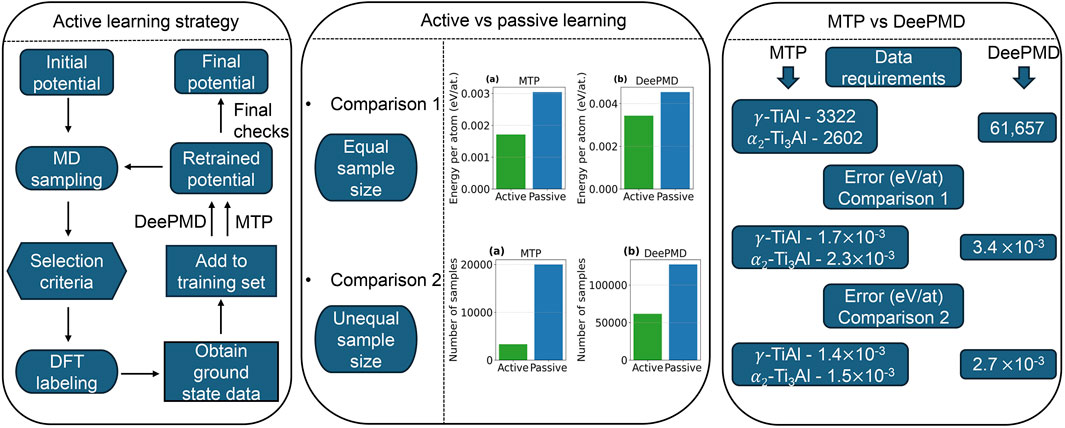
Figure 1. Graphical workflow of the study. The diagram outlines the active learning strategy implemented for both MTP and DeePMD and it illustrates the two levels of comparison between active and passive learning potentials. Sampling (MD simulations, Section 2.2, Section 2.3) generates diverse atomic configurations at the target thermodynamic conditions, while labeling (DFT calculations, Section 2.2, Section 2.3) assigns accurate energies and forces to those configurations. In Comparison 1, both potentials are trained using the same number of samples to directly evaluate their relative performance, while in Comparison 2, different sample sizes are used to achieve comparable error levels. The conclusion summarizes the comparisons in terms of data requirements and prediction accuracy of active learning potential for both methods.
2 Materials and methods
2.1 Dataset generation
The dataset generation began by constructing a series of unique structural configurations for
To generate the dataset, AIMD simulations were performed on these configurations using the Vienna ab-initio simulation (VASP). The AIMD calculations employed projector augmented wave (PAW) potentials (Blöchl, 1994) to accurately model electron-ion interactions, while exchange-correlation effects were treated via the generalized gradient approximation (GGA) using the Perdew–Burke–Ernzerhof (PBE) functional (Perdew et al., 1996; Perdew et al., 1997). An energy cutoff of 510 eV was adopted, with the Brillouin zone sampled by a
For active learning, short AIMD simulations were conducted at 300 K using the NVT ensemble (constant particle number, volume, and temperature) for 2.5 ps. These runs provided the initial training set for the DeePMD and MTP active learning models. The dataset containing the training and testing data for both MTP and DeePMD are available under the link: Active learning dataset. In contrast, the passive learning models were trained on the TiAlNb dataset from our previous work Chandran et al. (2024b), which comprises additional AIMD simulations carried out with both the NVT ensemble and the NPT (which maintains constant particle number, pressure, and temperature while allowing volume fluctuations) ensemble for approximately 10 ps across all configurations. For further details on the TiAlNb dataset, please refer to Chandran et al. (2024b).
For DeePMD potential training, the DeePMD-kit (Wang et al., 2018) was employed in conjunction with the LAMMPS package (Thompson et al., 2022) for MD simulations. Similarly, MTP potentials were trained using the MLIP package (Novikov et al., 2021), integrated with LAMMPS (Thompson et al., 2022) to streamline MD simulations. These tools facilitated efficient and accurate training for both DeePMD and MTP models.
2.2 Moment tensor potential (MTP) and active learning strategy
The theoretical foundation of MTP and its associated moment tensor descriptors has been extensively discussed in our previous work Chandran et al. (2024b) and in other publications Novikov et al. (2021), Podryabinkin et al. (2023). We refer the reader to these resources for a detailed understanding of these concepts. This section will concentrate on the active learning formulations concerning MTP.
Traditional methods for constructing interatomic potential training sets often involve manual trial-and-error. However, by defining extrapolation mathematically, this process can be automated. The D-optimality criterion (Novikov et al., 2021), which maximizes the information matrix, introduces an extrapolation grade, denoted as
The D-optimality criterion is particularly straightforward for linear regression, where MTP is parameterized by linear variables
Here
Each equation corresponds to a specific configuration. The D-optimality criterion selects
The extrapolation grade
where
If
with the corresponding row from
When the active set and the training set are the same, the parameters
Therefore, the energy of any configuration can be written as:
This mathematical formulation shows that MTP is extrapolating if
To extend the D-optimality criterion to MTP with nonlinear parameters, energies
Each row of this matrix corresponds to a specific configuration in the training set, while the matrix
To assess the effectiveness of our active learning strategy, we conducted two types of comparisons. In Comparison 1, we evaluated the performance of active versus passive learning using an identical number of training configurations, thereby isolating the impact of the learning strategy on model accuracy. In Comparison 2, we varied the dataset sizes to determine the number of configurations required by each approach to achieve comparable RMSEs. While working with MTP, we found that attempting to train a single active learning model for both
For each phase, we employed a consistent active learning workflow that comprises two main phases: sampling and labeling. During the sampling phase, MD simulations are performed using the initial potential (trained on a limited sample size) to explore the configuration space—the set of possible atomic arrangements and states of the system. Configurations where the model fails to accurately predict energies or forces are identified. In the labeling phase, these selected configurations are accurately annotated using DFT simulations, and the new data is incorporated into the training set, thereby refining the potential.
The initial training set comprised 170 configurations extracted from short NVT simulations of 2.5 ps at 300 K. We initiated the training with a 10.mtp (potential model with level 10) model and divided the active learning process into four steps. Steps 1, 2, and 3 corresponded to Comparison 1, using an equal number of samples for both learning strategies, while Step 4 extended the process for Comparison 2 by incorporating datasets of varying sizes. In step 1, MD simulations were conducted using the NVT ensemble at 300 K across different Nb concentrations, with iterations continuing until no new configurations were added to the training set. In Step 2, the exploration temperature range was expanded to 300 K, 500 K, 700 K, and 900 K, and the iterative process was repeated until no new configurations were chosen. In Step 3, we upgraded the model to 20.mtp, refined the k-point mesh to
For MD exploration, we utilized LAMMPS (Thompson et al., 2022), while VASP (Kresse and Furthmüller, 1996b; Kresse and Furthmüller, 199a) was employed for the ab initio calculations.
2.3 DeePMD and active learning strategy
The theoretical foundations of DeePMD have been discussed extensively in our previous work Chandran et al. (2024b) and elsewhere Zhang et al. (2019). Here, we focus on the active learning aspects. As with MTP, we performed two types of comparisons: in Comparison 1, we evaluated the performance of active versus passive learning using an identical number of training configurations; in Comparison 2, we varied the dataset sizes to determine how many configurations each approach requires to achieve comparable RMSEs. Unlike the MTP approach—where separate active learning processes were conducted for
For DeePMD, we began with a larger initial dataset of 40,000 configurations (20,000 for
During the sampling phase, MD simulations were conducted at 300 K, 500 K, 700 K, and 900 K using both the NVT and NPT ensembles for all Nb concentration cases across both phases. For Comparison 1, active learning iterations were performed over 80 cycles. The process began with 300 K NVT simulations, then transitioned to 300 K NPT simulations, with the number of simulation steps increasing as the iterations progressed, and eventually extending to higher temperatures. The production model of potential for Comparison 1 was obtained with a training run of 2
To assess the reliability of atomic force predictions, we used the concept of model deviation (Zhang et al., 2019), denoted as
Here,
Selected configurations exhibiting high model deviation were subsequently labeled using DFT simulations. These DFT calculations employed projector augmented wave (PAW) potentials (Blöchl, 1994) to accurately model electron–ion interactions, along with the generalized gradient approximation (GGA) (Perdew et al., 1996; Perdew et al., 1997) using the Perdew–Burke–Ernzerhof (PBE) functional. A cutoff energy of 510 eV and a k-spacing of 0.2
The DeePMD model architecture comprised radial and angular embedded-atom neural networks, each with three hidden layers containing 25, 50, and 100 nodes, respectively, to effectively capture complex interatomic interactions. Additionally, the fitting networks were constructed with three hidden layers of 240 nodes each. The training process began with an initial learning rate of 0.001, which was gradually reduced to
2.4 Simulated tension tests
To investigate the influence of Nb on the thermomechanical properties of the alloy, we performed uniaxial tension tests using MD models of both the
3 Results and discussion
3.1 Error analysis
This section presents the error analysis for the machine learning potentials developed for
3.1.1 MTP
Figures 2a–h presents the detailed error analysis for the active learning performed using MTP. Panels a, b, c, and d show the RMSEs for energy/atom and force for Comparison 1 and Comparison 2 in the
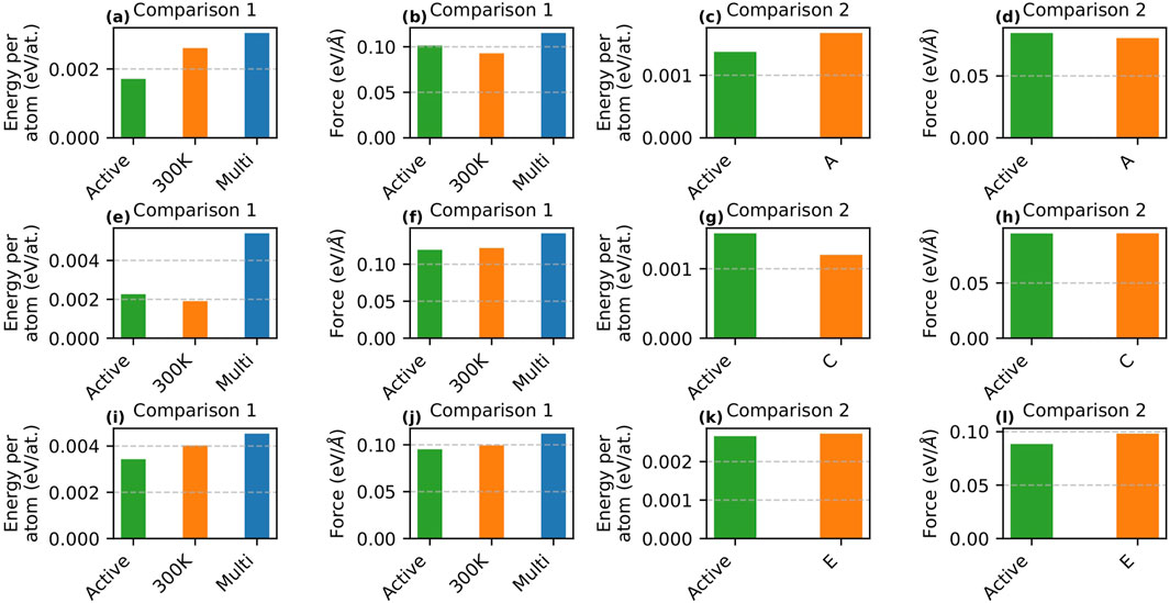
Figure 2. Comparison of RMSE energy/atom and force on the testing dataset during active learning using MTP and DeePMD. Panels (a–d) show MTP results for the
For the
To evaluate the effectiveness of the active learning strategy, we performed passive learning for Comparison 1 using 3,094 configurations under two scenarios. In the first scenario, only 300 K configurations were included in the training set to replicate the initial conditions of active learning. In the second scenario, configurations spanning a range of temperatures (300 K–900 K) were used. The RMSEs for energy/atom and force for all three cases (active learning, passive learning with 300 K configurations, and passive learning with multi-temperature configurations) are shown in Figures 2a,b. The results indicate that active learning achieved the lowest RMSE for energy/atom (
For Comparison 2, we examined whether a passive learning model trained on a larger dataset could match or exceed the predictive accuracy (in terms of RMSE) of active learning. At this stage, the active learning model was trained using 3,322 samples. Initially, passive learning was performed using Dataset-A (20,000 samples). Although the errors obtained from Dataset-A were comparable to those from active learning, we further investigated whether increasing the sample size with Dataset-B (80,000 samples) could reduce the error. Figures 2c,d compare the performance of active learning and passive learning using Dataset-A, while the RMSE values for Dataset-B are provided in Supplementary Table S1 in the supplementary section. Note that the passive learning models for Comparison 2 utilized a 24.mtp model. As shown in Figures 2c,d, active learning produced a lower RMSE for energy/atom (
For the
For Comparison 1, we compared active learning with passive learning using 1,665 configurations. The passive learning scenarios included both 300 K-only and multi-temperature samples. As shown in Figures 2e,f, active learning yielded a slightly higher RMSE for energy/atom (
For Comparison 2, passive learning was conducted using Dataset-C (comprising 20,000 samples), while active learning was performed with 2,602 samples. Similar to the
3.1.2 DeePMD
Here, we explore the comparison between active learning of DeePMD and passive learning using Comparison 1 and Comparison 2. The learning curves are presented in Supplementary Figure S2 in the supplementary section. Initially, we used 20,000 samples each from the
Figures 2i–l show the RMSEs for energy/atom and force for active learning potentials and their passive learning counterparts for Comparison 1 and Comparison 2, respectively. Similar to the case of MTP, for Comparison 1, we performed passive learning with the same number of samples as active learning (57,180 samples). Two scenarios were considered: one with only 300 K samples (matching the starting conditions of active learning) and the other with multi-temperature samples. The RMSE values for the active learning potential (RMSE energy/atom =
For Comparison 2, we conducted passive learning using Dataset-E, which comprises 127,212 samples. As in the MTP approach, although Dataset-E produced errors similar to those from active learning, we increased the sample size to create Dataset-F (333,340 samples) to examine whether a larger dataset would yield further error reduction. Note that active learning was performed using 61,657 samples. The RMSE comparisons are presented in Figures 2k,l, while the errors for Dataset-F are provided in Supplementary Table S1 in the supplementary section. The RMSE energy/atom values for active learning (
3.2 MD results
In this section, we summarize the results of MD simulations performed using the potentials derived from both active and passive learning. In Section 3.1, we assessed the RMSEs of the active and passive learning potentials under two scenarios—Comparison 1 and Comparison 2. Here, we present the MD simulation results obtained with these potentials to evaluate their effectiveness in predicting the fundamental material and thermo-mechanical properties of the two phases.
For Comparison 1, we utilized the passive learning potential trained on multi-temperature samples, which provides a fair comparison with active learning when exploring high-temperature properties. For Comparison 2, we selected the active learning cases using Dataset-A (
3.2.1 Energy volume curve and elastic constants
In this section, we evaluate the energy-volume (EV) curves obtained via the Murnaghan fit to compare the performance of passive and active learning. Figures 3, 4 display the EV curves for Comparison 1 and Comparison 2, respectively, alongside the corresponding DFT curves for MTP and DeePMD.
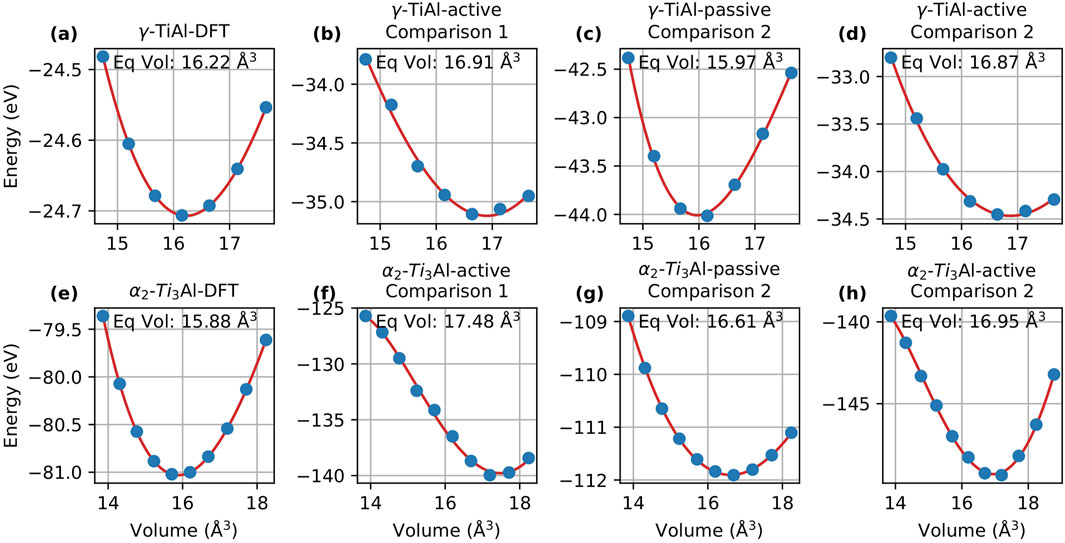
Figure 3. Energy-volume curves for
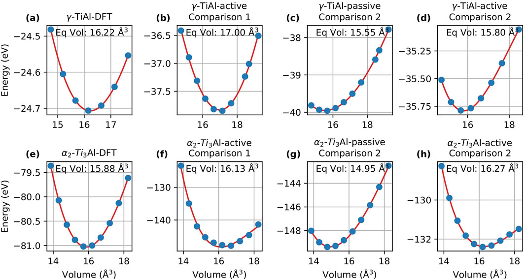
Figure 4. Energy-volume curves for
Here we focus on MTP. For Comparison 1, the passive learning potential failed to find a minimum volume, and therefore, the results for passive learning are not included here. For
For Comparison 2, the equilibrium volume for
When analyzing DeePMD, Figure 4 compares the EV curves for active and passive learning for both Comparison 1 and Comparison 2. Similar to the case of
In Comparison 2, the equilibrium volume predicted for
Along with evaluating equilibrium volume and lattice parameters, a comparative analysis of elastic constants was performed for both
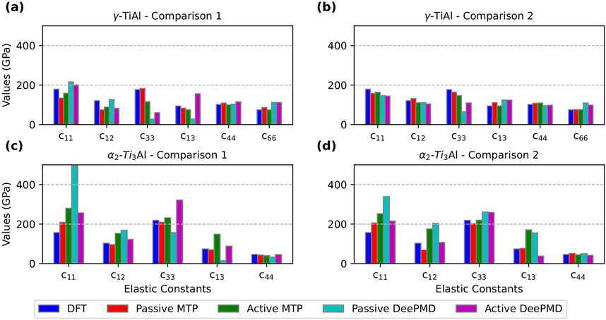
Figure 5. Comparison of elastic constants calculated using DFT, passive learning, and active learning potentials developed with MTP and DeePMD. (a,b) correspond to
For MTP, in the case of
For DeePMD, in the case of
Overall, active learning consistently demonstrated robust predictive capability for fundamental material properties—including lattice parameters, equilibrium volume, and elastic constants—compared to passive learning. However, passive learning exhibited greater variability and a tendency to overpredict, particularly in Comparison 1. It is also noteworthy that active learning produced some outliers, especially for the MTP active learning potential in
3.2.2 Finite temperature results
To evaluate the finite-temperature properties and compare the performance of active and passive learning for MTP and DeePMD, we computed the radial distribution functions (RDFs) and compared them with AIMD results. The RDFs were evaluated for both
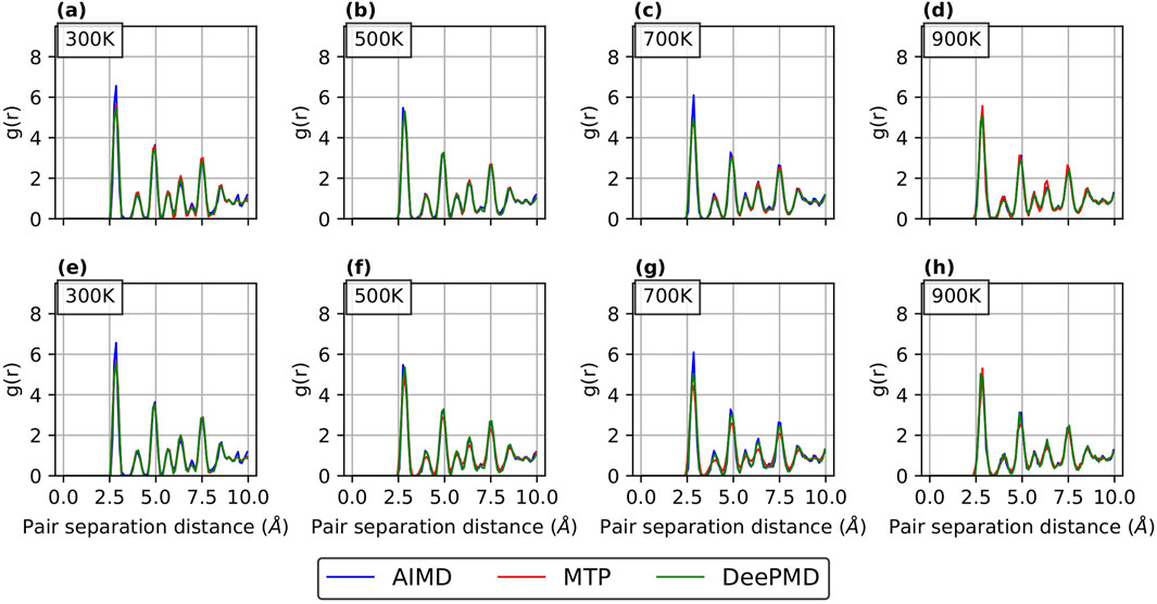
Figure 6. RDF curves for
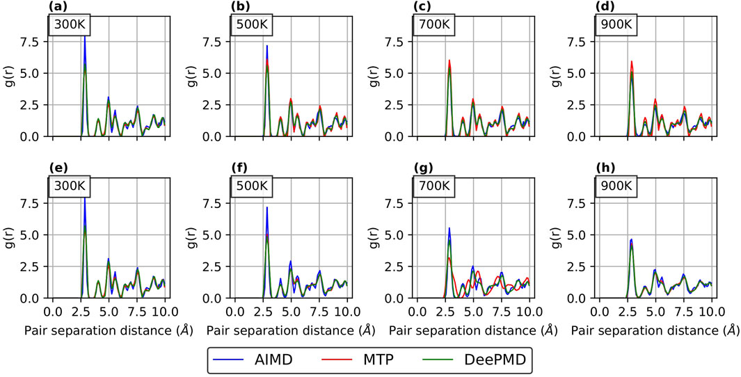
Figure 7. RDF curves for
RDFs provide a quantitative measure of how accurately a potential predicts the atomic arrangement in a material. In this study, RDFs were computed over a range of temperatures to evaluate the performance of the potentials from low to high temperatures. As shown in Figure 6 for
For Comparison 2 (refer Supplementary Figure S4; Supplementary Figure S5 in the supplementary section), the RDF curves show a good match with AIMD results for both passive and active learning. This is in line with our expectations, as our primary aim in Comparison 2 was to employ different sample sizes for active and passive learning while achieving comparable errors.
3.2.3 Tension tests and generalized stacking fault energy
In this study, we evaluated the performance of MTP and DeePMD potentials in capturing the thermo-mechanical behavior of our target phases (
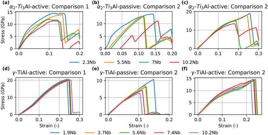
Figure 8. Stress-strain curves for
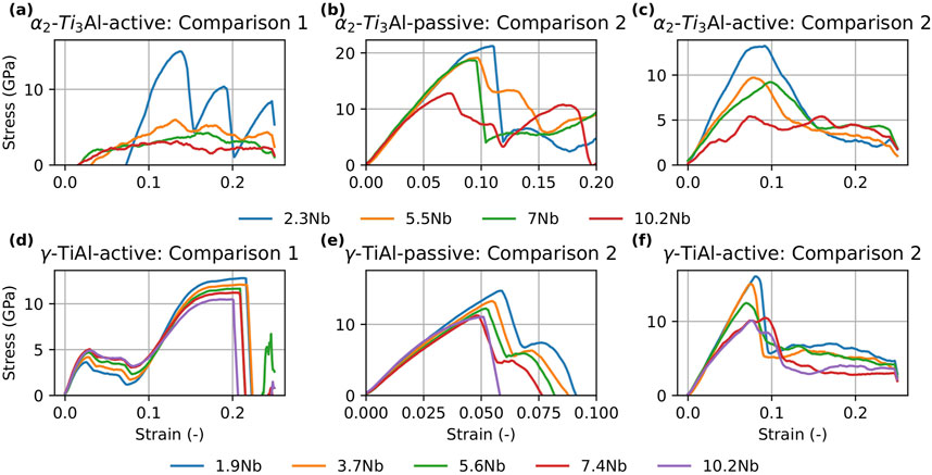
Figure 9. Stress-strain curves for
In addition to the tension tests, we computed the generalized stacking fault energy (GSFE) for both
For
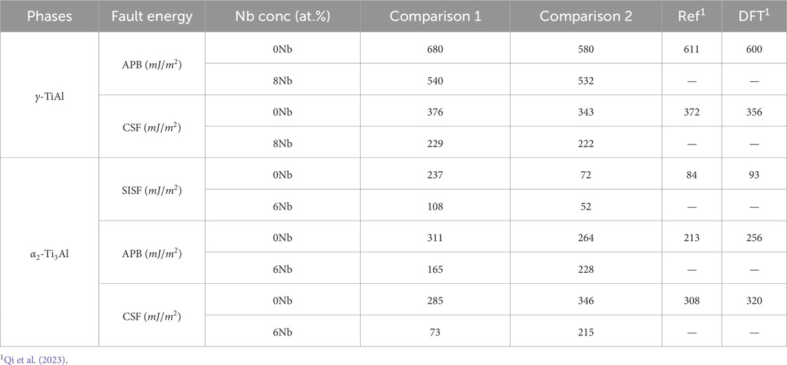
Table 1. Comparison of generalized stacking fault energy values for
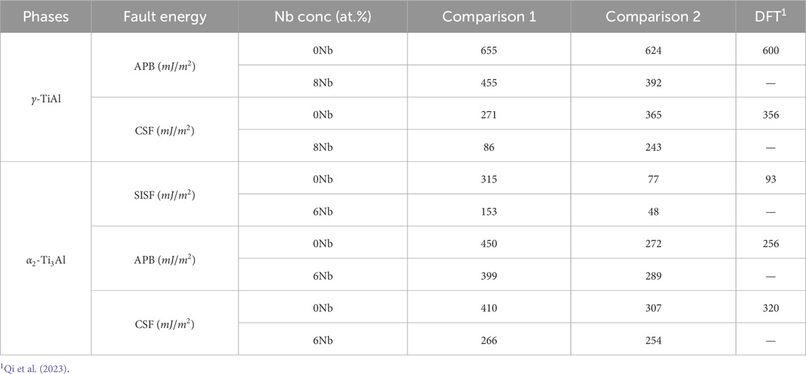
Table 2. Comparison of generalized stacking fault energy values for
Turning to the
In summary, the combined results of the tension tests and GSFE calculations suggest that Nb addition generally decreases the strength of both phases while simultaneously increasing ductility. These findings are in agreement with our previous work Chandran et al. (2024a), which demonstrated that Nb alloying enhances dislocation density and ductility at the cost of reduced strength.
4 Conclusion
In our study, we performed a comprehensive evaluation of passive and active learning strategies for developing interatomic potentials using both MTP and DeePMD methods. The analysis was structured into two stages. In Comparison 1, both approaches were trained on the same number of samples, allowing for a direct assessment of their performance on a fixed dataset. In Comparison 2, the number of training configurations was varied to determine how many samples are required to achieve comparable RMSE values for energy/atom and force. Under Comparison 1, the active learning potential outperformed the passive learning potential. In Comparison 2, where the primary goal was to achieve comparable accuracies for passive and active learning potentials, the active learning potentials required significantly fewer samples. Specifically, for MTP, the active learning potential used only 3,322 samples for
The MTP approach required separate potentials for
The predictive accuracy of the active learning potentials was further verified by comparing key material properties—such as elastic constants, equilibrium volume, and lattice parameters—against DFT results for both
Finite-temperature properties, as assessed using radial distribution functions, showed good agreement with AIMD for both phases, with slightly better results for
The accuracy and reliability of the developed potentials were validated through a comprehensive procedure. Accuracy was established by achieving low RMSEs on an independent test set and by good agreement of key physical properties like equilibrium volume, elastic constants, and GSFEs with reference DFT data. The potential’s reliability was confirmed by its ability to maintain thermal stability up to 900 K and to produce physically realistic stress-strain responses under large deformation. While some instabilities were observed, they were confined to the most demanding conditions: the
Finally, we acknowledge that the scope of this study was intentionally limited to defect free, single crystal models to isolate the properties of the
In summary, our study demonstrates that active learning provides a more efficient and accurate approach for interatomic potential development, significantly reducing data requirements and computational cost while maintaining robust predictive performance across various material properties and thermomechanical behaviors.
Data availability statement
The original contributions presented in the study are publicly available. This data can be found here: Zenodo under the link: https://zenodo.org/uploads/14990265
Author contributions
AC: Conceptualization, Data curation, Investigation, Methodology, Software, Writing – original draft, Resources. AS: Validation, Writing – review and editing. CP: Validation, Writing – review and editing. PJ: Validation, Writing – review and editing. RA: Investigation, Project administration, Supervision, Writing – review and editing, Validation. CC: Funding acquisition, Investigation, Project administration, Supervision, Writing – review and editing, Validation.
Funding
The author(s) declare that financial support was received for the research and/or publication of this article. The authors gratefully acknowledge funding by the
Conflict of interest
The authors declare that the research was conducted in the absence of any commercial or financial relationships that could be construed as a potential conflict of interest.
Generative AI statement
The author(s) declare that Generative AI was used in the creation of this manuscript. During the preparation of this work the author(s) used ChatGpt (ChatGpt 4o-mini) in order to improve the language and readability of the text. After using this tool/service, the author(s) reviewed and edited the content as needed and take(s) full responsibility for the content of the publication.
Publisher’s note
All claims expressed in this article are solely those of the authors and do not necessarily represent those of their affiliated organizations, or those of the publisher, the editors and the reviewers. Any product that may be evaluated in this article, or claim that may be made by its manufacturer, is not guaranteed or endorsed by the publisher.
Supplementary material
The Supplementary Material for this article can be found online at: https://www.frontiersin.org/articles/10.3389/fmats.2025.1591955/full#supplementary-material
References
Ángel, D. C., Xu, X., Gravelle, S., YazdanYar, A., Schmauder, S., and Fyta, M. (2023). Stability of binary precipitates in cu-ni-si-cr alloys investigated through active learning. Mater. Chem. Phys. 306, 128053. doi:10.1016/j.matchemphys.2023.128053
Appel, F., Oehring, M., and Paul, J. (2006). Nano-scale design of tial alloys based on β-phase decomposition. Adv. Eng. Mater. 8, 371–376. doi:10.1002/adem.200600013
Appel, F., Oehring, M., and Wagner, R. (2000). Novel design concepts for gamma-base titanium aluminide alloys. Intermetallics 8, 1283–1312. doi:10.1016/s0966-9795(00)00036-4
Appel, F., Paul, J. D. H., and Oehring, M. (2011). Gamma titanium aluminide alloys: science and Technology. John Wiley and Sons.
Attarian, S., Morgan, D., and Szlufarska, I. (2022). Thermophysical properties of flibe using moment tensor potentials. J. Mol. Liq. 368, 120803. doi:10.1016/j.molliq.2022.120803
Balyakin, I., and Sadovnikov, S. (2022). Deep learning potential for superionic phase of ag2s. Comput. Mater. Sci. 202, 110963. doi:10.1016/j.commatsci.2021.110963
Blöchl, P. E. (1994). Projector augmented-wave method. Phys. Rev. B 50, 17953–17979. doi:10.1103/physrevb.50.17953
Bock, F., Tasnádi, F., and Abrikosov, I. A. (2024). Active learning with moment tensor potentials to predict material properties: Ti0.5al0.5n at elevated temperature. J. Vac. Sci. and Technol. A, 42. doi:10.1116/6.0003260
Chandran, A., Ganesan, H., and Cyron, C. J. (2024a). Studying the effects of nb on high-temperature deformation in tial alloys using atomistic simulations. Mater. and Des. 237, 112596. doi:10.1016/j.matdes.2023.112596
Chandran, A., Santhosh, A., Pistidda, C., Jerabek, P., Aydin, R. C., and Cyron, C. J. (2024b). Comparative analysis of ternary tialnb interatomic potentials: moment tensor vs. deep learning approaches. Front. Mater. 11. doi:10.3389/fmats.2024.1466793
Chen, G., and Zhang, L. (2002). Deformation mechanism at large strains in a high-nb-containing tial at room temperature. Mater. Sci. Eng. A 329 (331), 163–170. doi:10.1016/s0921-5093(01)01554-4
Chen, H., Yuan, D., Geng, H., Hu, W., and Huang, B. (2023). Development of a machine-learning interatomic potential for uranium under the moment tensor potential framework. Comput. Mater. Sci. 229, 112376. doi:10.1016/j.commatsci.2023.112376
Cheng, L., Li, J., Xue, X., Tang, B., Kou, H., and Bouzy, E. (2016). Superplastic deformation mechanisms of high nb containing tial alloy with (α2 + γ) microstructure. Intermetallics 75, 62–71. doi:10.1016/j.intermet.2016.06.003
Cheng, Y., Wang, H., Wang, S., Gao, X., Li, Q., Fang, J., et al. (2021). Deep-learning potential method to simulate shear viscosity of liquid aluminum at high temperature and high pressure by molecular dynamics. AIP Adv. 11. doi:10.1063/5.0036298
Clemens, H., and Mayer, S. (2012). Design, processing, microstructure, properties, and applications of advanced intermetallic tial alloys. Adv. Eng. Mater. 15, 191–215. doi:10.1002/adem.201200231
Du, Y., Meng, Z., Yan, Q., Wang, C., Tian, Y., Duan, W., et al. (2022). Deep potential for a face-centered cubic cu system at finite temperatures. Phys. Chem. Chem. Phys. 24, 18361–18369. doi:10.1039/d2cp02758e
Dumitraschkewitz, P., Clemens, H., Mayer, S., and Holec, D. (2017). Impact of alloying on stacking fault energies in γ-tial. Appl. Sci. 7, 1193. doi:10.3390/app7111193
Farkas, D., and Jones, C. (1996). Interatomic potentials for ternary Nb - Ti - Al alloys. Model. Simul. Mater. Sci. Eng. 4, 23–32. doi:10.1088/0965-0393/4/1/004
Feng, T., and Lu, G. (2024). Hydration mgcl2-nacl-kcl molten salt using a novel approach for training machine learning potential. J. Mol. Liq. 394, 123533. doi:10.1016/j.molliq.2023.123533
Ghaffari, K., Bavdekar, S., Spearot, D. E., and Subhash, G. (2024). Validation workflow for machine learning interatomic potentials for complex ceramics. Comput. Mater. Sci. 239, 112983. doi:10.1016/j.commatsci.2024.112983
Gubaev, K., Podryabinkin, E. V., Hart, G. L., and Shapeev, A. V. (2019). Accelerating high-throughput searches for new alloys with active learning of interatomic potentials. Comput. Mater. Sci. 156, 148–156. doi:10.1016/j.commatsci.2018.09.031
Gubaev, K., Zaverkin, V., Srinivasan, P., Duff, A. I., Kästner, J., and Grabowski, B. (2023). Performance of two complementary machine-learned potentials in modelling chemically complex systems. npj Comput. Mater. 9, 129. doi:10.1038/s41524-023-01073-w
Guo, D., Li, C., Li, K., Shao, B., Chen, D., Ma, Y., et al. (2021). The thermoelectric performance of new structure snse studied by quotient graph and deep learning potential. Mater. Today Energy 20, 100665. doi:10.1016/j.mtener.2021.100665
He, R., Wu, H., Zhang, L., Wang, X., Fu, F., Liu, S., et al. (2022). Structural phase transitions in SrTio3 from deep potential molecular dynamics. Phys. Rev. B 105, 064104. doi:10.1103/physrevb.105.064104
Hirel, P. (2015). Atomsk: a tool for manipulating and converting atomic data files. Comput. Phys. Commun. 197, 212–219. doi:10.1016/j.cpc.2015.07.012
Holec, D., Reddy, R. K., Klein, T., and Clemens, H. (2016). Preferential site occupancy of alloying elements in tial-based phases. J. Appl. Phys. 119. doi:10.1063/1.4951009
Klein, T., Clemens, H., and Mayer, S. (2016). Advancement of compositional and microstructural design of intermetallic γ-tial based alloys determined by atom probe tomography. Materials 9, 755. doi:10.3390/ma9090755
Kresse, G., and Furthmüller, J. (1996a). Efficiency of ab-initio total energy calculations for metals and semiconductors using a plane-wave basis set. Comput. Mater. Sci. 6, 15–50. doi:10.1016/0927-0256(96)00008-0
Kresse, G., and Furthmüller, J. (1996b). Efficient iterative schemes forab initiototal-energy calculations using a plane-wave basis set. Phys. Rev. B 54, 11169–11186. doi:10.1103/physrevb.54.11169
Li, J., Liu, Y., Liu, B., Wang, Y., Zhao, K., and He, Y. (2014). Effect of nb particles on the flow behavior of tial alloy. Intermetallics 46, 22–28. doi:10.1016/j.intermet.2013.10.004
Li, T., Hou, Q., Cui, J.-c., Yang, J.-h., Xu, B., Li, M., et al. (2024). Deep learning interatomic potential for thermal and defect behaviour of aluminum nitride with quantum accuracy. Comput. Mater. Sci. 232, 112656. doi:10.1016/j.commatsci.2023.112656
Liu, P., Hou, B., Wang, A., Xie, J., and Wang, Z. (2022). Balancing the strength and ductility of ti2alc/tial composite with a bioinspired micro-nano laminated architecture. Mater. and Des. 220, 110851. doi:10.1016/j.matdes.2022.110851
Liu, Z., Lin, J., Li, S., and Chen, G. (2002). Effects of nb and al on the microstructures and mechanical properties of high nb containing tial base alloys. Intermetallics 10, 653–659. doi:10.1016/s0966-9795(02)00037-7
Lu, J., Wang, J., Wan, K., Chen, Y., Wang, H., and Shi, X. (2023). An accurate interatomic potential for the tialnb ternary alloy developed by deep neural network learning method. J. Chem. Phys. 158, 204702. doi:10.1063/5.0147720
Luo, Y., Meziere, J. A., Samolyuk, G. D., Hart, G. L. W., Daymond, M. R., and Béland, L. K. (2023). A set of moment tensor potentials for zirconium with increasing complexity. J. Chem. Theory Comput. 19, 6848–6856. doi:10.1021/acs.jctc.3c00488
Maruschak, P., Konovalenko, I., and Sorochak, A. (2023). Methods for evaluating fracture patterns of polycrystalline materials based on the parameter analysis of ductile separation dimples: a review. Eng. Fail. Anal. 153, 107587. doi:10.1016/j.engfailanal.2023.107587
Novikov, I. S., Gubaev, K., Podryabinkin, E. V., and Shapeev, A. V. (2021). The mlip package: moment tensor potentials with mpi and active learning. Mach. Learn. Sci. Technol. 2, 025002. doi:10.1088/2632-2153/abc9fe
Ouadah, O., Merad, G., and Abdelkader, H. S. (2021). Atomistic modelling of the γ-tial/α2-ti3al interfacial properties affected by solutes. Mater. Chem. Phys. 257, 123434. doi:10.1016/j.matchemphys.2020.123434
Ouadah, O., Merad, G., Saidi, F., Mendi, S., and Dergal, M. (2020). Influence of alloying transition metals on structural, elastic, electronic and optical behaviors of γ-tial based alloys: a comparative dft study combined with data mining technique. Mater. Chem. Phys. 242, 122455. doi:10.1016/j.matchemphys.2019.122455
Perdew, J. P., Burke, K., and Ernzerhof, M. (1996). Generalized gradient approximation made simple. Phys. Rev. Lett. 77, 3865–3868. doi:10.1103/physrevlett.77.3865
Perdew, J. P., Burke, K., and Ernzerhof, M. (1997). Generalized gradient approximation made simple [phys. rev. lett. 77, 3865 (1996)]. Phys. Rev. Lett. 78, 1396. doi:10.1103/physrevlett.78.1396
Podryabinkin, E., Garifullin, K., Shapeev, A., and Novikov, I. (2023). Mlip-3: active learning on atomic environments with moment tensor potentials. J. Chem. Phys. 159, 084112. doi:10.1063/5.0155887
Qi, J., Aitken, Z. H., Pei, Q., Tan, A. M. Z., Zuo, Y., Jhon, M. H., et al. (2023). Machine learning moment tensor potential for modeling dislocation and fracture in l10-TiAl and d019-ti3Al alloys. Phys. Rev. Mater. 7, 103602. doi:10.1103/physrevmaterials.7.103602
Rodriguez, A., Lam, S., and Hu, M. (2021). Thermodynamic and transport properties of lif and flibe molten salts with deep learning potentials. ACS Appl. Mater. and Interfaces 13, 55367–55379. doi:10.1021/acsami.1c17942
Rosenbrock, C. W., Gubaev, K., Shapeev, A. V., Pártay, L. B., Bernstein, N., Csányi, G., et al. (2021). Machine-learned interatomic potentials for alloys and alloy phase diagrams. npj Comput. Mater. 7, 24. doi:10.1038/s41524-020-00477-2
Song, L., Appel, F., Wang, L., Oehring, M., Hu, X., Stark, A., et al. (2020). New insights into high-temperature deformation and phase transformation mechanisms of lamellar structures in high nb-containing tial alloys. Acta Mater. 186, 575–586. doi:10.1016/j.actamat.2020.01.021
Song, Y., Yang, R., Li, D., Hu, Z., and Guo, Z. (2000). A first principles study of the influence of alloying elements on tial: site preference. Intermetallics 8, 563–568. doi:10.1016/s0966-9795(99)00164-8
Tasnádi, F., Bock, F., Tidholm, J., Shapeev, A. V., and Abrikosov, I. A. (2021). Efficient prediction of elastic properties of ti0.5al0.5n at elevated temperature using machine learning interatomic potential. Thin Solid Films 737, 138927. doi:10.1016/j.tsf.2021.138927
Thompson, A. P., Aktulga, H. M., Berger, R., Bolintineanu, D. S., Brown, W. M., Crozier, P. S., et al. (2022). Lammps - a flexible simulation tool for particle-based materials modeling at the atomic, meso, and continuum scales. Comput. Phys. Commun. 271, 108171. doi:10.1016/j.cpc.2021.108171
Wang, H., Zhang, L., Han, J., and E, W. (2018). Deepmd-kit: a deep learning package for many-body potential energy representation and molecular dynamics. Comput. Phys. Commun. 228, 178–184. doi:10.1016/j.cpc.2018.03.016
Wei, Y., Zhang, Y., Lu, G.-H., and Xu, H. (2012). Effects of transition metals in a binary-phase tial–ti3al alloy: from site occupancy, interfacial energetics to mechanical properties. Intermetallics 31, 105–113. doi:10.1016/j.intermet.2012.06.012
Wu, J., Zhang, Y., Zhang, L., and Liu, S. (2021). Deep learning of accurate force field of ferroelectric hfo2. Phys. Rev. B 103, 024108. doi:10.1103/physrevb.103.024108
Xu, T., Li, X., Wang, Y., and Tang, Z. (2023). Development of deep potentials of molten mgcl2–nacl and mgcl2–kcl salts driven by machine learning. ACS Appl. Mater. and Interfaces. doi:10.1021/acsami.2c19272
Zhang, H., Lu, D., Pei, Y., Chen, T., Zou, T., Wang, T., et al. (2023). Tensile behavior, microstructural evolution, and deformation mechanisms of a high nb-tial alloy additively manufactured by electron beam melting. Mater. and Des. 225, 111503. doi:10.1016/j.matdes.2022.111503
Zhang, L., Lin, D.-Y., Wang, H., Car, R., and E, W. (2019). Active learning of uniformly accurate interatomic potentials for materials simulation. Phys. Rev. Mater. 3, 023804. doi:10.1103/physrevmaterials.3.023804
Zhang, S., Zhang, C., Du, Z., Hou, Z., Lin, P., Kong, F., et al. (2016). Deformation behavior of high nb containing tial based alloy in α + γ two phase field region. Mater. and Des. 90, 225–229. doi:10.1016/j.matdes.2015.10.080
Zhao, Z., Yi, M., Guo, W., and Zhang, Z. (2024). General-purpose neural network potential for ti-al-nb alloys towards large-scale molecular dynamics with ab initio accuracy. Phys. Rev. B 110, 184115. doi:10.1103/PhysRevB.110.184115
Zhu, B., Xue, X., Kou, H., Li, X., and Li, J. (2018). Effect of microstructure on the fracture toughness of multi-phase high nb-containing tial alloys. Intermetallics 100, 142–150. doi:10.1016/j.intermet.2018.06.014
Keywords: TiAlNb alloy, machine-learning interatomic potentials, deep learning, moment tensor, active learning, molecular dynamics, density functional theory
Citation: Chandran A, Santhosh A, Pistidda C, Jerabek P, Aydin RC and Cyron CJ (2025) TiAlNb alloy interatomic potentials: comparing passive and active machine learning techniques with MTP and DeePMD. Front. Mater. 12:1591955. doi: 10.3389/fmats.2025.1591955
Received: 11 March 2025; Accepted: 08 July 2025;
Published: 30 July 2025.
Edited by:
Alireza Tabarraei, University of North Carolina at Charlotte, United StatesReviewed by:
Fuyang Tian, University of Science and Technology Beijing, ChinaPavlo Maruschak, Ternopil Ivan Pului National Technical University, Ukraine
Copyright © 2025 Chandran, Santhosh, Pistidda, Jerabek, Aydin and Cyron. This is an open-access article distributed under the terms of the Creative Commons Attribution License (CC BY). The use, distribution or reproduction in other forums is permitted, provided the original author(s) and the copyright owner(s) are credited and that the original publication in this journal is cited, in accordance with accepted academic practice. No use, distribution or reproduction is permitted which does not comply with these terms.
*Correspondence: Anju Chandran, YW5qdS5jaGFuZHJhbkBoZXJlb24uZGU=