Fuzzy Type RK4 Solutions to Fuzzy Hybrid Retarded Delay Differential Equations

1. Introduction

In this manuscript a system is modeled with the concept of retarded delay differential equation and we study it using fuzzy numbers. Nowadays hybrid systems play a vital role in communication systems and retard delay differential equation was considered to be unavoidable in modeling any biological models. In this paper these two separate mathematical concepts were combined under one roof called fuzzy. We call these system of differential equation as fuzzy hybrid retarded delay differential equations (FHRDDE).

The basic properties of fuzzy sets, fuzzy differential equations, fuzzy mappings were studied by various authors [1–7]. We recall that Pederson and Sambandham [8], Abbasbandy and Allahviranloo [9], Al Rawi et al. [10], Bellan and Zennaro [11], and Jayakumar et al. [12] have treated the hybrid, fuzzy, delay, fuzzy delay differential equation numerically, respectively. Prasantha Bharathi et al., studied various types of fuzzy delay differential equations in Prasantha Bharathi et al.[13, 14]. Different methods were used by some authors for solving Hybrid fuzzy differential equations without delay like [15] and [16]. Besides, L.C. Barros regularly studied fuzzy differential equations [15, 17–19]. In Pederson and Sambandham [8], the authors defined and solved the problem of hybrid fuzzy IVP. We extended this hybrid fuzzy IVP to fuzzy hybrid retarded delay IVP. In addition to that of hybrid term Λ(z_H(t)), the retarded delay term z_H(t − δ) is also used. So, there occurs some changes in the Runge-Kutta method which can be seen by comparing section 3 with Pederson and Sambandham [8].

The organization of the manuscript is given below. The section 2 treats the fuzzy hybrid retarded delay-differential systems. The section 3 shows the method of Runge-Kutta for fourth order (R-K-4) for dealing a FHRDDE and the section 4 holds algorithm and numerical example to prove the theory.

2. Fuzzy Hybrid Retarded Delay-Differential Systems

According to Al Rawi et al. [10] the retarded delay differential equations are defined in the form of a₀Dz_H(t) + b₀z_H(t) + b₁z_H(t − δ) = f(t). When f(t) = 0, it becomes homogeneous for every first order delay differential equation. Here we take f(t) as hybrid term and it was termed as hybrid retarded delay differential equations where the constants are given by a₀ = 1, b₀ = − 1, b₁ = − 1, f(t) = Λ(z_H(t)). Throughout the paper any function of the form f_H(t) represents the hybrid function satisfying the properties of fuzzy set proposed by Zadeh as followed by Pederson and Sambandham [8] defined over the hybrid term Λ(z_H(t)) and delay term z_H(t − δ).

Let us consider the following FHRDDE for α ∈ [0, 1]

$\begin{array}{ll}\{\begin{array}{l}D{z}_H(t)={[f(t,z_H(t),\Lambda (z_H(t)),z_H(t-\delta ))]}^{\alpha },t\ge t_0,\hfill \\ z_H(t)=\varphi (t),-\delta \le t\le t_0,\hfill \\ z_H(t_0)=z_0=\varphi (t_0),\hfill \end{array}& (1)\end{array}$

where Λ(z_H(t)) is the hybrid function and z_H(t − δ) is the delay function involving the delay term δ. More over the Hybrid function is the function involving two or more sub functions acting differently in specific interval defined over the main functions interval. i.e., The sub functions of main function acts differently in the different sub intervals of main function's domain. In the numerical example below, we have taken the hybrid function Λ(z_H(t)) = m(t).Λ(z(t)) where m(t) and Λ(z(t)) will vary for different values defined over the interval t ∈ [t₀, t_n]. The delay term δ varies in the interval (t₀, t_n]. z_H(t) = ϕ(t) is the initial function and z_H(t₀) = z₀ = ϕ(t₀) is the initial value defined at t₀. It is obvious that

$\begin{array}{l}D{z}_H(t)={\left[f(t,\varphi (t),\Lambda (z_H(t)),z_H(t-\delta ))\right]}^{\alpha },\\ -\delta \le t\le t_0,0\le \alpha \le 1.\end{array}$

It follows that for ${\left[f(t,z_H(t),\Lambda (z_H(t)),z(t-\delta ))\right]}^{\alpha }$. Now we can define the above fuzzy valued function Dz_H(t) i.e., ${\left[f(t,z_H(t),\Lambda (z_H(t)),z_H(t-\delta ))\right]}^{\alpha }$ as follows

$\begin{array}{l}{\left[f(t,z_H(t),\Lambda (z_H(t)),z_H(t-\delta ))\right]}^{\alpha }\\ =\{\begin{array}{l}\min f(t,v_H(t),\Lambda (v_H(t)),v_H(t-\delta )):\hfill \\ v_H(t)\in ({\underset{\_}{z}}_H{(t)}^{\alpha },{\overline{z}}_H{(t)}^{\alpha }),\hfill \\ \Lambda (v_H(t))\in (\Lambda ({\underset{\_}{z}}_H{(t)}^{\alpha }),\Lambda ({\overline{z}}_H{(t)}^{\alpha })),\hfill \\ v_H(t-\delta )\in ({\underset{\_}{z}}_H{(t-\delta )}^{\alpha },{\overline{z}}_H{(t-\delta )}^{\alpha }),\hfill \\ \max f(t,v_H(t),\Lambda (v_H(t)),v_H(t-\delta )):\hfill \\ v_H(t)\in ({\underset{\_}{z}}_H{(t)}^{\alpha },{\overline{z}}_H{(t)}^{\alpha }),\hfill \\ \Lambda (v_H(t))\in (\Lambda ({\underset{\_}{z}}_H{(t)}^{\alpha }),\Lambda ({\overline{z}}_H{(t)}^{\alpha })),\hfill \\ v_H(t-\delta )\in (\underset{\_}{z}{(t-\delta )}^{\alpha },{\overline{z}}_H{(t-\delta )}^{\alpha }),\hfill \end{array}& (2)\end{array}$

for z_H ∈ E with α- level sets ${\left[z_H\right]}^{\alpha }=\left[{\underset{\_}{z}}_H^{\alpha },{\overline{z}}_H^{\alpha }\right],0\le \alpha \le 1$

$\begin{array}{ll}\{\begin{array}{l}D({\underset{\_}{z}}_H^{\alpha })(t)=\min (f(t,v_H(t),\Lambda (v_H(t)),v(t-\delta )):\hfill \\ v_H(t)\in ({\underset{\_}{z}}_H{(t)}^{\alpha },{\overline{z}}_H{(t)}^{\alpha }),\Lambda (v_H(t))\hfill \\ \in (\Lambda ({\underset{\_}{z}}_H{(t)}^{\alpha }),\Lambda ({\overline{z}}_H{(t)}^{\alpha }))\hfill \\ v_H(t-\delta )\in ({\underset{\_}{z}}_H{(t-\delta )}^{\alpha },{\overline{z}}_H{(t-\delta )}^{\alpha })),\hfill \\ D({\overline{z}}_H^{\alpha })(t)=\max (f(t,v_H(t),\Lambda (v_H(t)),v_H(t-\delta )):\hfill \\ v_H(t)\in ({\underset{\_}{z}}_H{(t)}^{\alpha },{\overline{z}}_H{(t)}^{\alpha }),\Lambda (v_H(t))\hfill \\ \in (\Lambda ({\underset{\_}{z}}_H{(t)}^{\alpha }),\Lambda ({\overline{z}}_H{(t)}^{\alpha })),\hfill \\ v_H(t-\delta )\in ({\underset{\_}{z}}_H{(t-\delta )}^{\alpha },{\overline{z}}_H{(t-\delta )}^{\alpha })).\hfill \end{array}& (3)\end{array}$

for t ∈ I and 0 ≤ α ≤ 1.

3. Fourth-Order Fuzzy Type Runge-Kutta Method (R-K-4)

We recall that the R-K-4 plays a vital role in solving differential equations. Also, it holds good for any dynamical system involving delay differential equations. We use the R-K-4 for a FHRDDE (1). Here we use a new simplified form of R-K-4. We define

$\begin{array}{l}{\underset{\_}{z}}_{t_{n+1};\alpha }-{\underset{\_}{z}}_{t_n;\alpha }={\displaystyle \sum _{j=1}^4{w}_i}{\underset{\_}{K}}_j(t_n;z_H(t_n;\alpha ),\\ {\overline{z}}_{t_{n+1};\alpha }-\overline{z}{t}_n;\alpha ={\displaystyle \sum _{j=1}^4{w}_i}{\overline{K}}_j(t_n;z_H(t_n;\alpha )),\end{array}$

where w₁, w₂, w₃, and w₄ are simple constants and

$\begin{array}{l}{K}_j=(min{R}_j,max{R}_j),j=1,2,3,4.\\ R_j=hf(t,v_H(t),\Lambda (v_H(t)),v_H(t-\delta ),),j=1.\\ R_j=hf\left(t+\frac{h}{2},v_H(t),\Lambda (v_H(t)),v_H(t-\delta ),\right),j=2,3.\\ R_j=hf(t+h,v_H(t),\Lambda (v_H(t)),v_H(t-\delta ),),j=4.\end{array}$

Such that,

$\begin{array}{l}{v}_H(t)\in \left[{\underset{\_}{z}}_H(t_{k,n};\alpha ),{\overline{z}}_H(t_{k,n};\alpha )\right],j=1.\\ v_H(t)\in \left[{\underset{\_}{N}}_{j-1},{\overline{N}}_{j-1}\right],j=2,3,4.\\ v_H(t-\delta )\in \left[{\underset{\_}{z}}_H(t_{k,n}-\delta ;\alpha ),{\overline{z}}_H(t_{k,n}-\delta ;\alpha )\right],j=1.\\ v_H(t-\delta )\in \left[{\underset{\_}{N}}_{j-1},{\overline{N}}_{j-1}\right],j=2,3,4.\\ v_H(t_l)\in \left[{\underset{\_}{z}}_H(t_{k,0};\alpha ),{\overline{z}}_H(t_{k,0};\alpha )\right],j=1,2,3,4.\end{array}$

where,

$\begin{array}{lll}{N}_j& =& z+\frac{K_j}{2},j=1,2.\\ N_j& =& z+K_j,j=3.\end{array}$

$N_j\in \left({\underset{\_}{N}}_j(t_{k,n},z_H(t_{k,n};\alpha )),{\overline{N}}_j(t_{k,n},z(t_{k,n};\alpha ))\right),$

$K_j\in \left({\underset{\_}{K}}_j(t_{k,n}{\underset{\_}{z}}_H(t_{k,n};\alpha )),{\overline{K}}_j(t_{k,n},z(t_{k,n};\alpha ))\right),$

$Z\in \left({\underset{\_}{z}}_H(t_{k,n};\alpha ),\overline{z}(t_{k,n};\alpha )\right).$

Next we define the followings

$\begin{array}{l}P={\underset{\_}{K}}_1(t,z_H(t;\alpha ))+2{\underset{\_}{K}}_2(t,z_H(t;\alpha ))+2{\underset{\_}{K}}_3(t,z_H(t;\alpha ))\\ +{\underset{\_}{K}}_4(t,z_H(t;\alpha )),\\ \\ Q={\overline{K}}_1(t,z_H(t;\alpha ))+2{\overline{K}}_2(t,z_H(t;\alpha ))+2{\overline{K}}_3(t,z_H(t;\alpha ))\\ +{\overline{K}}_4(t,z_H(t;\alpha )).\end{array}$

The exact solution at t_{n + 1} is given by

$\begin{array}{ll}\{\begin{array}{c}{\underset{\_}{Z}}_H(t_{n+1};\alpha )={\underset{\_}{Z}}_H(t_n;\alpha )+\frac{P}{6},\\ {\overline{Z}}_H(t_{n+1};\alpha )={\overline{Z}}_H(t_n;\alpha )+\frac{Q}{6}.\end{array}& (4)\end{array}$

The approximate solution has the following form

$\begin{array}{ll}\{\begin{array}{c}{\underset{\_}{z}}_H(t_{n+1};\alpha )\approx {\underset{\_}{z}}_H(t_n;\alpha )+\frac{P}{6},\\ {\overline{z}}_H(t_{n+1};\alpha )\approx {\overline{z}}_H(t_n;\alpha )+\frac{Q}{6}.\end{array}& (5)\end{array}$

where P and Q are given by

$P=P\left[(t_n,{\underset{\_}{Z}}_H(t_n;\alpha ),{\overline{Z}}_{H_n}(t;\alpha ))\right]$

and

$Q=Q\left[(t_n,{\underset{\_}{Z}}_H(t_n;\alpha ),{\overline{Z}}_{H_n}(t;\alpha ))\right],$

respectively.

4. Algorithm and the Numerical Example

This section consists of an algorithm followed by an example to understand the proposed theory.

Algorithm (R-K-4):

Step:1 Fix N=10,

Step:2 Calculate h by $h=\frac{(t_n-t_0)}{t_n*N}$

Step:3 Set t_i = i*h for i = 0, 1, …, n and compute z(t_i).

Step:4 Take t₀ as initial point and z₀ as the initial value.

Step:5 Compute K₁, K₂, K₃, K₄, z(t_i) using Runge-Kutta method, explained in previous section.

Step:6 Calculate the upcoming iterations using z(t_i+1) = z(t_i) as described in previous section.

Step:7 Repeat the steps, Step:2, Step:4 and Step:5 for t_i ≤ t_n.

Step:8 Quit the process at t_i > t_n.

The Numerical Example

Consider the FHRDDE, extended from Pederson and Sambandham [8], namely

$\begin{array}{ll}\{\begin{array}{ll}D{z}_H(t)={[z_H(t)+\Lambda (z_H(t))+z(t-1)]}^{\alpha },\hfill & 0\le t\le 3,0\le \alpha \le 1,\hfill \\ z_H(t)=[(\frac{6}{8}+\frac{4\alpha }{8})e^t,(\frac{9}{8}-\frac{\alpha }{8})e^t],\hfill & -1\le t\le 0.\hfill \end{array}& (6)\end{array}$

The hybrid function is defined as Λ(z_H(t)) = m(t).Λ(z(t)) as mentioned in section 2 where,

$\begin{array}{l}m(t)=\left|sin(\pi .t)\right|,fort\in [0,3].\\ \Lambda (\nu (t))=\{\begin{array}{l}0,\text{ \hspace{1em}for }t=0,\hfill \\ \nu ,\text{\hspace{1em} for }t\in (0,3].\hfill \end{array}\end{array}$

Then the above Equation (6)

$\begin{array}{ll}\{\begin{array}{ll}D{z}_H(t)={[z_H(t)+m(t)\Lambda (z(t))+z(t-1)]}^{\alpha },\hfill & 0\le t\le 3,0\le \alpha \le 1,\hfill \\ z_H(t)=[(\frac{6}{8}+\frac{4\alpha }{8})e^t,(\frac{9}{8}-\frac{\alpha }{8})e^t],\hfill & -1\le t\le 0.\hfill \end{array}& (7)\end{array}$

The exact solution of (7) is given by

$\begin{array}{l}{Z}_H\left(t;\alpha \right)=\\ \{\begin{array}{ll}[\left(\frac{6}{8}+\frac{4\alpha }{8}\right)e^t,\left(\frac{9}{8}+\frac{\alpha }{8}\right)e^t],\hfill & t\in [-1,0],\hfill \\ [\left(\frac{6}{8}+\frac{4\alpha }{8}\right)e^{t-1}-\frac{e\cos \left(\pi t\right)}{\pi }-\frac{1}{e}+\frac{e}{\pi }+1,\hfill \\ (\frac{9}{8}+\frac{\alpha }{8})e^{t-1}-\frac{e\cos \left(\pi t\right)}{\pi }-\frac{1}{e}+\frac{e}{\pi }+1],\hfill & t\in [0,1],\hfill \\ [\left(\frac{6}{8}+\frac{4\alpha }{8}\right)(-\frac{t}{e}+\frac{et}{\pi }+t+e^{t-2}+\hfill \\ \frac{e\sin \left(\pi t\right)}{{\pi }^2}-\frac{e\cos \left(\pi t\right)}{\pi }-\frac{1}{e}+1),\hfill \\ (\frac{9}{8}+\frac{\alpha }{8})(-\frac{t}{e}+\frac{et}{\pi }+t+e^{t-2}+\hfill \\ \frac{e\sin \left(\pi t\right)}{{\pi }^2}-\frac{e\cos \left(\pi t\right)}{\pi }-\frac{1}{e}+1\left)\right],\hfill & t\in [1,2],\hfill \\ [\left(\frac{6}{8}+\frac{4\alpha }{8}\right)\hfill \\ \left(\frac{1}{2}\right(-\frac{t^2}{e}+\frac{e{t}^2}{\pi }+t^2-\frac{2et}{\pi }+2e^{t-3}+\frac{2e\sin \left(\pi t\right)}{{\pi }^2}\hfill \\ -\frac{2e\left({\pi }^2-1\right)\cos \left(\pi t\right)}{{\pi }^3}-\frac{4}{e}+\frac{4e}{\pi }-\frac{2e}{{\pi }^3}+4\left)\right),\hfill \\ (\frac{9}{8}+\frac{\alpha }{8})\hfill \\ \left(\frac{1}{2}\right(-\frac{t^2}{e}+\frac{e{t}^2}{\pi }+t^2-\frac{2et}{\pi }+2e^{t-3}+\frac{2e\sin \left(\pi t\right)}{{\pi }^2}\hfill \\ -\frac{2e\left({\pi }^2-1\right)\cos \left(\pi t\right)}{{\pi }^3}-\frac{4}{e}+\frac{4e}{\pi }-\frac{2e}{{\pi }^3}+4\left)\right],\hfill & t\in [2,3],\hfill \end{array}& \left(8\right)\end{array}$

where $Z_H(t;\alpha )=\left[\underset{\_}{Z_H}(t;\alpha ),\overline{Z_H}(t;\alpha )\right].$

Let $z_H(n;\alpha )=\left[\underset{\_}{z_H}(n;\alpha ),\overline{z_H}(n;\alpha )\right]$ and,

$\begin{array}{l}{A}_1=c_0{\displaystyle \sum _{s=0}^{2n}(e^{(-1+\frac{sh}{2})})},A_2=c_0{\displaystyle \sum _{s=0}^{2n}(HSin(}\frac{sh\pi }{2})),B_1=c_1{\displaystyle \sum _{s=1}^{20}(e^{(-1+\frac{sh}{2})})},\\ B_2=c_2{\displaystyle \sum _{s=20}^{2n}{e}^{(-2+\frac{sh}{2})}},B_3=(\frac{(n-10)H}{\pi }),B_4=c_2{\displaystyle \sum _{s=20}^{2n}(}\frac{(HCos(\frac{sh\pi }{2})}{\pi })),\\ B_5=c_3{\displaystyle \sum _{s=1}^{2n}(HSin(}\frac{sh\pi }{2})),D_1=c_1{\displaystyle \sum _{s=1}^{20}(e^{(-1+\frac{sh}{2})})},D_2=c_4{\displaystyle \sum _{s=20}^{40}(e^{(-2+\frac{sh}{2})})},\\ D_3=c_5{\displaystyle \sum _{s=40}^{2n}(e^{(-3+\frac{sh}{2})})},D_4=(\frac{(30-n)H}{\pi }),D_5=c_2{\displaystyle \sum _{s=20}^{2n}(}\frac{(HCos(\frac{sh\pi }{2})}{\pi })),\\ D_6=c_3{\displaystyle \sum _{s=1}^{2n}(HSin(}\frac{sh\pi }{2})),D_7=c_6{\displaystyle \sum _{s=40}^{2n}(}\frac{(HSin(\frac{sh\pi }{2})}{{\pi }^2})),\end{array}$

The approximate solution is given by

$\begin{array}{l}{z}_H\left(n;\alpha \right)=\\ \{\begin{array}{ll}[\left(\frac{6}{8}+\frac{4\alpha }{8}\right),\left(\frac{9}{8}+\frac{\alpha }{8}\right)],\hfill & (-10\le n\le 0),\hfill \\ [\left(\frac{6}{8}+\frac{4\alpha }{8}\right)(z_0+h(A_1+A_2)),\hfill \\ (\frac{9}{8}+\frac{\alpha }{8})(z_0+h(A_1+A_2))],\hfill & (1\le n\le 10),\hfill \\ [\left(\frac{6}{8}+\frac{4\alpha }{8}\right)\hfill \\ (z_0+h(n-10)-\frac{h}{6e}(6n-1)+h({\displaystyle \sum _{i=1}^5{B}_i})),\hfill \\ (\frac{9}{8}+\frac{\alpha }{8})\hfill \\ (z_0+h(n-10)-\frac{h}{6e}(6n-1)+h({\displaystyle \sum _{i=1}^5{B}_i}))],\hfill & (11\le n\le 20),\hfill \\ [\left(\frac{6}{8}+\frac{4\alpha }{8}\right)(z_0+((h^2(\frac{n^2-(400)}{2}))(1-\frac{1}{e}+\frac{H}{\pi }))\hfill \\ +h(10-\frac{59}{6e})+h{\displaystyle \sum _{i=1}^7(D_i)}),\hfill \\ (\frac{9}{8}+\frac{\alpha }{8})(z_0+((h^2(\frac{n^2-(400)}{2}))(1-\frac{1}{e}+\frac{H}{\pi }))\hfill \\ +h(10-\frac{59}{6e})+h{\displaystyle \sum _{i=1}^7(D_i)})],\hfill & (21\le n\le 30),\hfill \end{array}& (9)\end{array}$

where the coefficients are written as

$\begin{array}{l}\begin{array}{ll}{c}_0=\{\begin{array}{l}1/6,s=0,2n.\hfill \\ 2/3,s=1,3,\mathrm{...},2n-1.\hfill \\ 1/3,s=2,4,\mathrm{...},2n-2.\hfill \end{array}\hfill & c_1=\{\begin{array}{l}1/6,s=20.\hfill \\ 2/3,s=1,3,\mathrm{...},19.\hfill \\ 1/3,s=2,4,\mathrm{...},18.\hfill \end{array}\hfill \\ c_2=\{\begin{array}{l}1/6,s=20,2n.\hfill \\ 2/3,s=21,23,\mathrm{...},2n-1.\hfill \\ 1/3,s=22,24,\mathrm{...},2n-2.\hfill \end{array}\hfill & c_3=\{\begin{array}{l}1/6,s=2n\hfill \\ 2/3,s=1,3,\mathrm{...},2n-1.\hfill \\ 1/3,s=2,4,\mathrm{...},2n-2.\hfill \end{array}\hfill \\ c_4=\{\begin{array}{l}1/6,s=20,40.\hfill \\ 2/3,s=21,23,\mathrm{...},39.\hfill \\ 1/3,s=22,24,\mathrm{...},38.\hfill \end{array}\hfill & c_5=\{\begin{array}{l}1/6,s=40,2n\hfill \\ 2/3,s=41,43,\mathrm{...},2n-1.\hfill \\ 1/3,s=42,44,\mathrm{...},2n-2.\hfill \end{array}\hfill \end{array}\\ c_6=\{\begin{array}{l}-1/6,s=40,2n.\hfill \\ -2/3,s=41,43,\mathrm{...},2n-1.\hfill \\ -1/3,s=42,44,\mathrm{...},2n-2.\hfill \end{array}\end{array}$

Consider another $H={(1+h+\frac{h^2}{2}+\frac{h^3}{6},\frac{h^4}{24})}^{10},$ t ∈ [t₀, t_n], i.e., t ∈ [0, 3], h = 0.1 Set n = 10t and z_H(10t) = z_H(n).

5. Conclusion

We have used the R-K-4 method to find the numerical solution of FHRDDE. We presented the Table 1 only for t = 3, h = 0.1 for α ∈ [0, 1]. The values of z_H for t ∈ [0, 3] are plotted in Figure 1 for α = 1 and in Figure 3 for α ∈ [0, 3]. The comparison of the solutions represented in Figure 1 for non-fuzzy IVP and the Figure 2 for fuzzy IVP prove the accuracy of R-K-4 with that of the exact solution. From the Table 1 we can conclude that the accuracy of the method proposed is about four decimal places. Also if we increase the order of the Runge-Kutta method the accuracy of our numerical solutions will increase. The analytical and numerical results obtained by this paper ensures the hybrid system with time lag (delay) can be solved. Thus, we can solve properly any FHRDDE using the R-K-4 method. We followed [10] to write the retarded delay differential equation in regular homogeneous form and we added a hybrid term to make it as non-homogenous equation which in turn makes our governing Equation 1 as the hybrid fuzzy retarded delay differential equation. Thus, our results differ from results on the delay papers like [11, 12] or as in hybrid papers like [8, 20]. There are differences between the traditional Runge-Kutta methods presented in Pederson and Sambandham [8] and the reported method because in our case the Runge-Kutta method involves both hybrid and retarded delay term. The previously published papers varies only the hybrid term in regular intervals. However, we constructed a system in which both hybrid term Λ(z_H(t)) and delay term z_H(t − δ) are subject to vary in some regular intervals. We also generalized the numerical solution which will provide very closer solution for any values in the given intervals. In the above example, we have taken $(\frac{6}{8}+\frac{4\alpha }{8})$ and $(\frac{9}{8}-\frac{\alpha }{8})$ as our fuzzy numbers. But one can choose different fuzzy numbers with in the interval α ∈ [0, 1]. In all the cases the non-member, partial member and the full member of both approximate and analytical solution will coincide as they are defined in [0 ≤ α ≤ 1]. According to our knowledge the researchers working with the numerical solutions of hybrid systems like [8, 20] did not considered the system with time lag. In this paper we solved the hybrid system with time lag and we open a gate for the related future research in areas like communication systems and signal processing.

TABLE 1

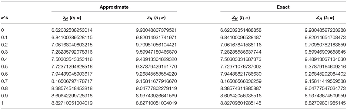
Table 1. Comparing the exact and the approximate solution.

FIGURE 1

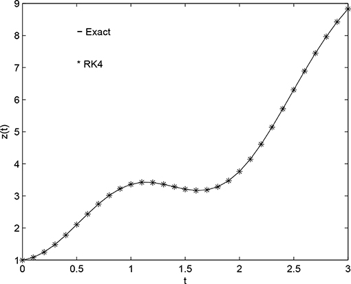
Figure 1. Comparing approximate solution with the exact solution (for h = 0.1, α = 1 at t ∈ [0, 3]).

FIGURE 2

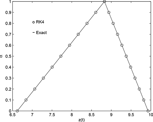
Figure 2. Comparing the approximate solution with the exact solution (for h = 0.1, α ∈ [0, 1] at t = 3).

FIGURE 3

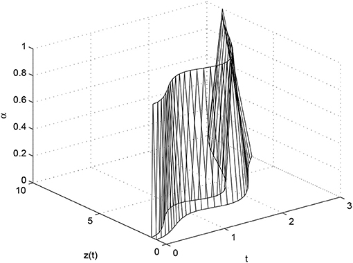
Figure 3. Approximate solution by R-K-4 (for h = 0.1, α ∈ [0, 1] for t ∈ [0, 3]).

Data Availability Statement

All datasets generated for this study are included in the article/supplementary material.

Author Contributions

PD formulated the problem, converted it into fuzzy functions, and solved the problem analytically. DB solved the problem numerically and carefully proof-read the whole paper. JT generalized both numerical and exact solutions. VS plotted all the three graphs for various values. All the authors equally typeset their parts in the journal template and checked the final version of the manuscript.

Conflict of Interest

The authors declare that the research was conducted in the absence of any commercial or financial relationships that could be construed as a potential conflict of interest.

Acknowledgments

The authors would like to thank the reviewers for their kind suggestions toward the improvement of the paper.

References

1. Goetschel R, Voxman W. Elementary fuzzy calculus. Fuzzy Sets Syst. (1986) 18:31–43. doi: 10.1016/0165-0114(86)90026-6

CrossRef Full Text | Google Scholar

2. Kaleva O. Fuzzy differential equations. Fuzzy Sets Syst. (1987) 24:301–17. doi: 10.1016/0165-0114(87)90029-7

CrossRef Full Text | Google Scholar

3. Bukley JJ, Feuring T. Fuzzy differential equations. Fuzzy Sets Syst. (2000) 110:43–54.

Google Scholar

4. Seikkala S. On the fuzzy initial value problem. Fuzzy Sets Syst. (1987) 24:319–30. doi: 10.1016/0165-0114(87)90030-3

CrossRef Full Text | Google Scholar

5. Lupulescu V. On a class of fuzzy functional differential equations. Fuzzy Sets Syst. (2009) 160:1547–62. doi: 10.1016/j.fss.2008.07.005

CrossRef Full Text | Google Scholar

6. Dubois D, Prade H. Towards fuzzy differential calculus, Part 3. Differentiation. Fuzzy Sets Syst. (1982) 8:225–33. doi: 10.1016/S0165-0114(82)80001-8

CrossRef Full Text | Google Scholar

7. Chang SL, Zadeh LA. On fuzzy mapping and control. IEEE Trans Syst Man Cybern. (1972) 2:30–4. doi: 10.1109/TSMC.1972.5408553

CrossRef Full Text | Google Scholar

8. Pederson S, Sambandham M. The Runge-Kutta method for hybrid fuzzy differential equations. Nonlinear Anal Hybrid Syst.(2008) 2:626–34. doi: 10.1016/j.nahs.2006.10.013

CrossRef Full Text | Google Scholar

9. Abbasbandy S, Allahviranloo T. Numerical solution of fuzzy differential equation by Runge-Kutta Method. Nonlinear Stud. (2004) 11:117–29.

Google Scholar

10. AL Rawi SN, Salih RS, Mohammed AA. Numerical Solution of N^th order linear delay differential equation using Runge-Kutta method. Um Salama Sci J. (2006) 3:140–6.

Google Scholar

11. Bellen A, Zennaro M. Numerical methods for delay differential equations. In: Golub GH, Schwab CH, Light WA, Suli E, editors. Numerical Mathematics and Scientific Computation. Oxford: Oxford Science Publications; Clarendon Press (2003). p. 1–10; 63-70.

Google Scholar

12. Jayakumar T, Parivallal A, Prasantha Bharathi D. Numerical solutions of Fuzzy delay differential equations by fourth order Runge Kutta Method. Adv Fuzzy Sets Syst. (2016) 21:135–61. doi: 10.17654/FS021020135

CrossRef Full Text | Google Scholar

13. Prasantha Bharathi D, Jayakumar T, Vinoth S. Numerical solution of fuzzy pure multiple retarded delay differential equations. Int J Res Advent Technol. (2018) 6:3693–8.

Google Scholar

14. Prasantha Bharathi D, Jayakumar T, Vinoth S. Numerical solution of fuzzy pure multiple neutral delay differential equations. Int J Adv Sci Res Manage. (2019) 4:172–8.

Google Scholar

15. Paripour M, Hajilou E, Hajilou A, Heidari H. Application of Adomian decomposition method to solve hybrid fuzzy differential equations. J Taibah Univ Sci. (2015) 9:95–103. doi: 10.1016/j.jtusci.2014.06.002

CrossRef Full Text | Google Scholar

16. Sepahvandzadeh A, Ghazanfari B. Variational Iteration Method for solving Hybrid Fuzzy differential equation. J Math Extens. (2016) 10:76–85.

Google Scholar

17. de Barros LC, Pedro FS. Fuzzy differential equations with interactive derivative. Fuzzy Sets Syst. (2017) 309:64–80. doi: 10.1016/j.fss.2016.04.002

CrossRef Full Text | Google Scholar

18. Barros LC, Gomes LT, Tonelli PA. Fuzzy differential equations: an approach via fuzzification of the derivative operator. Fuzzy Sets Syst. (2013) 230:39–52. doi: 10.1016/j.fss.2013.03.004

CrossRef Full Text | Google Scholar

19. Mizukoshi MT, Barros LC, Chalco-Cano Y, Roman-Flores H, Bassanezi RC. Fuzzy differential equations and the extension principle. Inform Sci. (2007) 177:3627–35. doi: 10.1016/j.ins.2007.02.039

CrossRef Full Text | Google Scholar

20. Sambandham M. Perturbed Lyapunov-like functions and hybrid fuzzy differential equations. Int J. Hybrid Syst. (2002) 2:23–34.

Google Scholar