Flavor Techniques for LFV Processes: Higgs Decays in a General Seesaw Model

1. Introduction

Lepton flavor violating (LFV) processes are optimal observables to test new physics hypotheses. This is particularly true for LFV transitions in the charged sector, as they are forbidden in the Standard Model (SM), and extremely suppressed if one minimally introduces the observed light neutrino masses. Consequently, any observation of charged LFV transition would be a clear evidence of new physics beyond the SM (BSM). Moreover, since in several BSM theories this kind of processes are induced via quantum corrections with new particles running in the loops, exploring LFV transitions in the intensity frontier allows us to probe the existence of these new particles even if they are too heavy to be directly produced in any other experiment.

Many BSM theories are constructed following the same steps that succeed in the case of the SM. First, we write the most general Lagrangian with the chosen symmetries and field content, which includes some parameters that we may consider as the fundamental parameters of the theory. The easiest way of doing this is by choosing a field basis in which the conservation of the symmetries, in particular the gauge symmetries, is explicit, implying in most of the cases that gauge interaction are diagonal in this basis and that some particles are massless. Therefore, we refer to this basis as the interaction basis in general, and also as gauge or flavor basis for the particular cases of gauge or fermionic fields, respectively. As a second step, we assume that some of these gauge symmetries are spontaneously broken to a smaller gauge symmetry group, as in the case of the electroweak symmetry breaking (EWSB), providing masses to some of the fields. Nevertheless, these new mass terms do not need to be diagonal in the interaction basis, and some non-diagonal terms may appear, mixing different interaction fields. The basis in which the mass terms are diagonal is called the mass or physical basis, since it is in this basis where the parameters could be directly related to observables. The relation between the two basis is given by a series of unitary rotation matrices. In some simple cases, we may be able to find analytical expressions for these rotation matrices in terms of the original parameters in the interaction basis, however this is not always possible and we often need to use numerical methods.

The physical basis is the natural choice to compute any transition in quantum field theory (QFT), since we can properly define a loop expansion for any observable, such as the LFV processes we mentioned before. The reason is that, in this basis, particles have well-defined propagators, meaning that they will keep their identity unless they interact with other two– or more– particles. The resulting expressions will be given in terms of the physical parameters, i.e., physical masses and rotation matrices. Nevertheless, in many cases it is desirable to have expressions that, albeit approximate, are given directly in terms of the fundamental parameters of the interaction basis. Indeed, this is particularly interesting in the case of flavor transitions, since we can often track its origin back to few parameters in the original Lagrangian, e.g., the non-diagonal Yukawa couplings in many models.

One possibility in order to obtain expressions in terms of the fundamental parameters is to compute the amplitudes first in the physical basis, and then expand them using the relations between the two basis. An interesting possibility in this direction is given by the Flavor Expansion Theorem [1, 2], which provides a recipe to translate analytically the expression in the mass basis to the flavor basis. Unfortunately, this technique may suffer from limitations when the external momenta and the masses within the loops are such that the involved loop integrals suffer from branch cuts [1]. As this will be the case for the observable we will be interested in, we will not consider this technique any further. We refer to the original references for more details.

Alternatively, we will use another technique, the so-called mass insertion approximation (MIA), which is very powerful when computing flavor transitions. The main idea behind this technique is to perform a new computation, independent to that in the physical basis, working directly in the interaction basis. In general, the mass matrices will not be diagonal in this basis and the non-diagonal terms will provide two-point interactions, the so-called mass insertions, which will allow a particle to transform into another one along its propagation. Then, the propagator of a particle is understood as successive insertions of this kind and, therefore, this technique provides a diagrammatic expansion of any observable. Although computing the full series of mass insertions would reproduce the complete result in the physical basis, in general this is not possible to do. Nevertheless, in the case where the mass insertions are small—smaller than the diagonal mass terms—, we can treat these insertions perturbatively and compute the diagrams in the interaction basis to a given order in the MIA expansion. For this reason, the MIA technique is very useful to compute LFV processes, since the strong experimental bounds suggest that any kind of parameter leading to LFV transitions should be small.

In order to show the applicability of the MIA for computing flavor transitions, we apply it here to the case of LFV Higgs decays (LFVHD). The motivation to choose these observables is the strong experimental effort that both ATLAS and CMS are doing in the search for this kind of decays, which we summarize in Table 1 with the current upper bounds. Furthermore, the LHCb collaboration has also performed similar searches [6]. From the theoretical side, these observables have also been studied very actively, exploring their potential to probe BSM theories such as neutrino mass models [7–15], minimal flavor violation [16–19], supersymmetric models [20–38], two Higgs doublet models [39–43], composite Higgs models [44], models with extra dimensions [45–48], effective Lagrangians [49–54] and many others [55–68]. Indeed, some of these works used the MIA technique for computing the LFVHD rates [13, 33].

TABLE 1

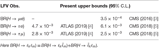
Table 1. Present experimental upper bounds on lepton flavor violating Higgs boson decays.

The particular model we will choose to perform the MIA computations will be a general type-I seesaw model [69–73], where an arbitrary number of right-handed (RH) neutrinos are added to the SM. This kind of models are very well motivated from the observation of neutrino oscillations [74–77], and it is well-known that they may lead to sizable LFV transitions, see for instance the recent review [78] and references therein. Furthermore, it has been shown that the MIA works very well in this context [13, 79].

The paper is organized as follows. We start by describing the basics for a MIA computation in section 2, providing two simple examples with the explicit computations in the case of small and large mass insertions. Then, in section 3 we apply this technique to the case of the LFV Higgs decays in a general seesaw model. We use it to derive an effective vertex in the case of heavy RH neutrinos, which helps to compare the results with current experimental bounds from other observables and to conclude on maximum allowed LFVHD rates. Finally, we conclude in section 4. Further details on the computation and heavy mass expansions are provided in the Appendices.

2. Basics for a Mass Insertion Approximation Computation

In many models, spontaneous symmetry breaking is behind particle masses. It leads to quadratic terms in the Lagrangian, which implies a mass matrix in the interaction basis. In general, this matrix is non-diagonal and when it is diagonalized the physical basis is derived. This latter basis is in general the chosen basis to perform QFT computations, as it is possible to properly define a loop expansion for a given observable. Nevertheless, when doing this one usually loses track of the parameters in the interaction basis. On the other hand, having analytical expressions for a given observable in terms of the fundamental parameters of the theory, it is possible to extract information about them from the experimental measurements directly.

In order to work with the fundamental parameters in the computation of a given observable, the mass insertion approximation provides a powerful tool. This method is a diagrammatic diagonalization of the mass matrix in the interaction basis: in this approach the diagonal entries are considered as the mass parameters, while the non-diagonal ones are interpreted as two-point interactions (the so-called mass insertions) of the corresponding states. In this context, the propagator of a given state is constructed from the successive mass insertions connecting two different fields and the interaction states are dressed with these consecutive interactions. The exact diagonalization corresponds to a complete resummation of the infinite mass insertions that can occur in the propagation. In general, it is not possible to do this exact resummation, and therefore an approximation is used: as in a Taylor expansion, a dimensionless parameter is defined as the ratio of the non-diagonal mass insertion over the diagonal mass parameter, and its magnitude defines how many mass insertions must be taken into account to achieve a given precision in the expansion. In a general model, the hierarchy between the different mass scales defines different dimensionless parameters.

In this section, we present two examples as an illustration of the application of this technique. The first one corresponds to a situation in which the non-diagonal terms are smaller that the diagonal ones. Then we show that the first two terms in the MIA expansion reproduce the computation in the physical mass basis to that order. The second example represents the opposite situation: the non-diagonal parameters are larger than the diagonal ones, and we need to perform a complete resummation of the infinite mass insertions.

2.1. First Example: Small Mass Insertions

As a first example of the MIA application, we consider a toy-model composed of three real scalar fields ρ, Φ₁ and Φ₂ in the interaction basis, with the following the Lagrangian:

$\begin{array}{l}{{L}}_{\text{gauge}}=\frac{1}{2}{({\partial }_{\mu }\rho )}^2-\frac{1}{2}{\mu }_{\rho }^2{\rho }^2+\frac{1}{2}{({\partial }_{\mu }{\mathbf{\Phi }}_I)}^2\\ -\frac{1}{2}{M}_{IJ}^2{\mathbf{\Phi }}_I{\mathbf{\Phi }}_J-{\mathbf{\lambda }}_{IJ}{\mathbf{\Phi }}_I{\mathbf{\Phi }}_J\rho ,& (1)\end{array}$

with an implicit sum over I, J is understood.

For simplicity, we assume a real and symmetric squared mass matrix but not aligned in the interaction space:

$\begin{array}{ll}{\text{M}}^2=\left(\begin{array}{cc}{M}^2& m^2\\ m^2& M^2\end{array}\right),& (2)\end{array}$

and a cubic interaction between the scalar ρ with the Φ fields that is diagonal in interaction space:

$\begin{array}{ll}\lambda =\left(\begin{array}{cc}\lambda & 0\\ 0& \lambda \end{array}\right).& (3)\end{array}$

The mass matrix M² can be diagonalized by an orthogonal matrix O:

$\begin{array}{ll}{\varphi }_i={\text{O}}_{Ii}{\Phi }_I\Rightarrow {\text{O}}^T{\text{M}}^2\text{O}=\text{diag}(M_{+}^2,M_{-}^2),& (4)\end{array}$

defining a physical basis ϕ_±, with physical masses given by

$\begin{array}{ll}{M}_{\pm }^2=M^2\pm m^2.& (5)\end{array}$

Therefore, the Lagrangian in the physical basis is:

$\begin{array}{l}{{L}}_{\text{phys}}=\frac{1}{2}{({\partial }_{\mu }\rho )}^2-\frac{1}{2}{\mu }_{\rho }^2{\rho }^2+\frac{1}{2}{({\partial }_{\mu }{\varphi }_{+})}^2-\frac{1}{2}{M}_{+}^2{\varphi }_{+}^2\\ +\frac{1}{2}{({\partial }_{\mu }{\varphi }_{-})}^2-\frac{1}{2}{M}_{-}^2{\varphi }_{-}^2-\lambda ({\varphi }_{+}^2\rho +{\varphi }_{-}^2\rho ).& (6)\end{array}$

Let us consider the one-loop contributions to the self-energy of the ρ scalar field: in the physical basis, they come from the Lagrangian of Equation (6) and correspond to the sunset topology of Figure 1, with ϕ_± running in the loop. They are expressed as function of the one-loop integrals defined in Appendix 1:

$\begin{array}{l}-i\Pi (q)={\displaystyle \int \frac{d^{D}k}{{(2\pi )}^D}}(-i\lambda )\frac{i}{k^2-M_{+}^2}(-i\lambda )\frac{i}{{(k+q)}^2-M_{+}^2}\\ +(M_{+}\to M_{-})\\ =\frac{i}{16{\pi }^2}{\lambda }^2(B_0(q,M_{+},M_{+})+B_0(q,M_{-},M_{-})).& (7)\end{array}$

FIGURE 1

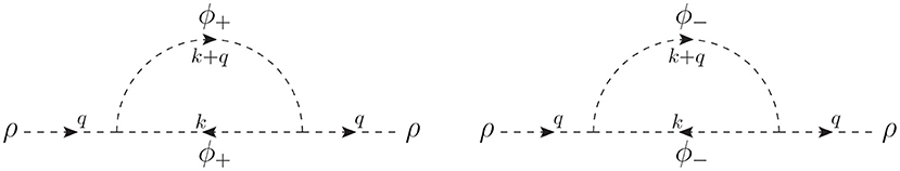
Figure 1. One-loop contributions to the self-energy of the scalar ρ in the physical basis, corresponding to the Lagrangian of Equation (6).

Notice that, in this example, the matrix O is not involved in the computation in the physical basis. This is due to the simplicity of our model, where we assumed λ = λ $\mathbb{1}$ and therefore O is not present in Equation (6). In a more general case, the expressions in the physical basis are given terms of the physical masses and the rotation matrices.

In order to illustrate how the MIA works, we assume that the non-diagonal entry in the mass matrix M² of Equation (2) is much smaller than the diagonal one. Then the dimensionless parameter m²/M² ≪ 1 is defined and it controls the diagrammatic expansion in the interaction basis. Now, considering the interaction fields Φ_{1, 2} of Equation (1) running in the loop with an associated mass parameter M and the two-point interaction $~m^2{\Phi }_1{\Phi }_2$ as the mass insertion, the systematic procedure is to add successive mass insertions up to a given order. In Figure 2, the first two contributions in the MIA are shown: they correspond, respectively, to the leading order (LO) with no mass insertions, and to the next to leading order (NLO) with two insertions. In this example we cannot close the loop with an odd number of mass insertions in the sunset topology, since the cubic interactions are diagonal. Notice that all these MIA diagrams are at the same loop level, that of the corresponding diagrams in the physical basis, however they are of different order in the MIA expansion. Therefore, in this approach we have an expansion for the self-energy at the one-loop level as

$\begin{array}{ll}-i{\Pi }^{\text{MIA}}(q)=-i{\Pi }_{\text{LO}}^{\text{MIA}}(q)-i{\Pi }_{\text{NLO}}^{\text{MIA}}(q)+\dots & (8)\end{array}$

where the dots are contributions with more mass insertions and, thus, suppressed by higher powers of the dimensionless parameter m²/M².

FIGURE 2

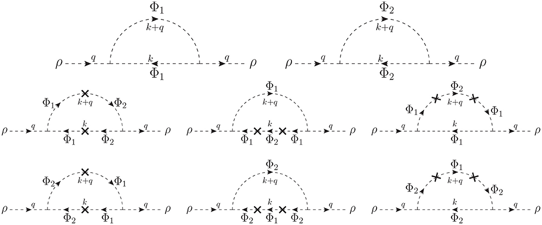
Figure 2. One-loop contributions to the self-energy of the scalar ρ in the interaction basis. The first row corresponds to the LO in the MIA calculation (there is no mass insertion), while the second and third rows define the NLO (there are two mass insertions denoted by crosses).

The LO contribution in the MIA has the same type of diagrams than in the physical mass basis, but the interaction states Φ_{1, 2} are running in the loop now. Then,

$\begin{array}{ll}-i{\Pi }_{\text{LO}}^{\text{MIA}}(q)=\frac{i}{16{\pi }^2}2{\lambda }^2{B}_0(q,M,M).& (9)\end{array}$

On the other hand, there are six diagrams contributing to the NLO order in the MIA. Each one has two mass insertion, so they are proportional to m⁴. Explicitly, the one-loop integral for the middle-left diagram in Figure 2 is given by,

$\begin{array}{l}\int \frac{d^{D}k}{{(2\pi )}^D}(-i\lambda )\frac{i}{k^2-M^2}\left(-i{m}^2\right)\frac{i}{k^2-M^2}\\ (-i\lambda )\frac{i}{{(k+q)}^2-M^2}\left(-i{m}^2\right)\frac{i}{{(k+q)}^2-M^2}\\ =\frac{i}{16{\pi }^2}{\lambda }^2{m}^4{D}_0(0,q,0,M,M,M,M).& (10)\end{array}$

Then, the NLO contribution in the MIA is:

$\begin{array}{l}-i{\Pi }_{\text{NLO}}^{\text{MIA}}(q)=\frac{i2{\lambda }^2{m}^4}{16{\pi }^2}[D_0(0,q,0,M,M,M,M)\\ +D_0(0,0,q,M,M,M,M)+D_0(q,0,0,M,M,M,M)]\\ =-\frac{i}{16{\pi }^2}\frac{4{\lambda }^2{m}^4}{q^2-4M^2}\left(\frac{1}{M^2}+2\frac{\log \left(\frac{2M^2-q^2+\sqrt{q^2(q^2-4M^2)}}{2M^2}\right)}{\sqrt{q^2(q^2-4M^2)}}\right).& (11)\end{array}$

The analytical comparison between the MIA and the physical basis results is obtained when the physical masses (and the matrix rotations if any) are expressed in terms of the gauge parameters and the physical basis expressions are expanded up to a given order. In this example, since we have used the MIA up to two insertions, we need to expand the expression in the physical basis up to ${O}(m^4/M^4)$. From Equations (5) and (7), the physical basis computation of the scalar ρ self-energy in terms of the gauge interaction parameters is

$\begin{array}{l}-i\Pi \left(q\right)=\frac{i}{16{\pi }^2}{\lambda }^2(B_0\left(q,\sqrt{M^2+m^2},\sqrt{M^2+m^2}\right)\\ +B_0\left(q,\sqrt{M^2-m^2},\sqrt{M^2-m^2}\right)).& (12)\end{array}$

This two-point B₀ one-loop function, participating also in the LO contribution of the MIA in Equation (9), is given by

$\begin{array}{l}{B}_0\left(q,w,w\right)=\frac{2}{4-D}-{\gamma }_E+\log \left(\frac{4\pi {\mu }^2}{w^2}\right)+2\\ +\frac{\sqrt{q^2(q^2-4w^2)}\log \left(\frac{2w^2-q^2+\sqrt{q^2(q^2-4w^2)}}{2w^2}\right)}{q^2},& (13)\end{array}$

where γ_E is the Euler-Mascheroni constant and μ is the usual scale for dimensional regularization.

We can now expand the expression obtained in the physical basis, Equation (12), under the assumption of m² ≪ M². At zero order, m = 0, this equation trivially leads to the LO MIA contribution in Equation (9). The next terms in the expansion are of order m⁴/M⁴, and lead to the NLO MIA expression in Equation (11). Similarly, one could check that higher order terms m⁸/M⁸, m¹²/M¹², …  will correspond to higher order terms in the MIA expansion with 4, 6, …  insertions.

We remark again that the simplicity of the present toy-model allows us to compare explicitly the MIA results with the expansion of the physical basis results, due to the analytical diagonalization of the 2 × 2 mass matrix. In a more complex situation, this diagonalization is only performed numerically, and thus the dependence on the interaction parameters is missed. Moreover, the computational effort could be huge for higher dimension mass matrices. In that context, the MIA diagrammatic computation is a powerful tool in order to work with the interaction parameters explicitly. As we said, the MIA results correspond to a perturbative calculation in a dimensionless parameter.

2.2. Second Example: Large Mass Insertions

Now we analyze a situation in which a non-diagonal entry of the mass matrix is larger than a diagonal one, i.e., the corresponding dimensionless parameter results larger than 1. In that case, an exact resummation of this large mass insertion is needed. In particular, we consider a Dirac spinor ψ = P_Lψ + P_Rψ = ψ_L + ψ_R with mass M and momentum p. The corresponding quadratic terms of the free Dirac Lagrangian are

$\begin{array}{lll}{{L}}_D& =& \bar{\psi }\cancel{p}\psi -M\bar{\psi }\psi \\ & =& \overline{{\psi }_L}\cancel{p}{P}_L{\psi }_L+\overline{{\psi }_R}\cancel{p}{P}_R{\psi }_R-\overline{{\psi }_L}M{P}_L{\psi }_L-\overline{{\psi }_R}M{P}_R{\psi }_R\\ & =& (\overline{{\psi }_L}\overline{{\psi }_R})\left(\begin{array}{cc}\cancel{p}{P}_L& -M{P}_R\\ -M{P}_L& \cancel{p}{P}_R\end{array}\right)\left(\begin{array}{c}{\psi }_L\\ {\psi }_R\end{array}\right),& (14)\end{array}$

where we have a matrix of dimension 2 in chiral space (P_{L, R} = (I ∓ γ₅)/2). This approach is equivalent to having two massless fermions ψ_L and ψ_R interacting through the mass insertion M. The corresponding massless propagators are the inverse of the kinetic terms:

$\begin{array}{ll}{\text{Prop}}_{{\psi }_L}=\frac{i\cancel{p}}{p^2}{P}_R\text{ and }{\text{Prop}}_{{\psi }_R}=\frac{i\cancel{p}}{p^2}{P}_L.& (15)\end{array}$

As before, the dimensionless parameter of the MIA expansion should be the ratio between the mass insertion M and the mass of the fermions. However, the latter is zero in this example, implying an infinitely large expansion parameter. This fact can be solved by defining a dressed propagator that accounts for a resummation of all the insertions of this kind. In the chiral basis, there are four types of propagators depending on the chiralities of the connected fermions (LL, LR, RL, and RR), as showed in Figure 3. Here, the thin lines represent the massless propagators, the blacks dots are the mass insertions and the thick lines correspond to the dressed propagators (after the resummation of the successive two point interactions). The dressed propagators that connect two fermions with the same chirality contain an even number of mass insertions, while the ones connecting two opposite chiralities have an odd number of mass insertions.

FIGURE 3

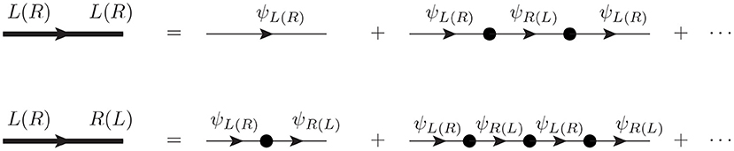
Figure 3. Diagrammatic interpretation of the dressed propagators (thick lines) for the same and opposite chiralities as an infinite series of successive mass insertions (black dots) between two massless propagators (thin lines).

Explicitly, the propagator connecting two left-handed fermions (LL) corresponds to the geometric series:

$\begin{array}{lll}{\text{Prop}}_{L\to L}& =& \frac{i\cancel{p}}{p^2}{P}_R+\frac{i\cancel{p}}{p^2}{P}_R(-iM{P}_R)\frac{i\cancel{p}}{p^2}{P}_L(-iM{P}_L)\frac{i\cancel{p}}{p^2}{P}_R+\cdots \\ & =& \frac{i\cancel{p}}{p^2}{\displaystyle \sum _{n\ge 0}}{\left(\frac{M^2}{p^2}\right)}^n{P}_R=\frac{i\cancel{p}}{p^2-M^2}{P}_R,& (16)\end{array}$

and the propagator connecting two right-handed fermions (RR) is obtained with the interchange P_L ↔ P_R:

$\begin{array}{ll}{\text{Prop}}_{R\to R}=\frac{i\cancel{p}}{p^2-M^2}{P}_L.& (17)\end{array}$

In the same way, the propagator connecting opposite chiralities (LR) comes from the geometric series:

$\begin{array}{l}{\text{Prop}}_{L\to R}=\frac{i\cancel{p}}{p^2}{P}_L(-iM{P}_L)\frac{i\cancel{p}}{p^2}{P}_R+\frac{i\cancel{p}}{p^2}{P}_L(-iM{P}_L)\frac{i\cancel{p}}{p^2}{P}_R(-iM{P}_R)\\ \frac{i\cancel{p}}{p^2}{P}_L(-iM{P}_L)\frac{i\cancel{p}}{p^2}{P}_R+\cdots =\frac{iM}{p^2}{\displaystyle \sum _{n\ge 0}}{\left(\frac{M^2}{p^2}\right)}^n{P}_R\\ =\frac{iM}{p^2-M^2}{P}_R,& (18)\end{array}$

and the propagator RL results from the LR after interchanging P_L ↔ P_R:

$\begin{array}{ll}{\text{Prop}}_{R\to L}=\frac{iM}{p^2-M^2}{P}_L.& (19)\end{array}$

From the previous relations, we can interpret that the successive non-diagonal two-point interactions dress the propagator providing the corresponding masses. It is important to connect this approach with four types of propagators with the standard one of the Dirac propagator $\frac{i(\cancel{p}+M)}{p^2-M^2}$: in a generic process with a Dirac propagator, the MIA approach produces four diagrams with the LL, LR, RL and RR propagators. Adding these contributions from Equations (16–19), the complete Dirac propagator is restored. This procedure works in a generic context of two interacting states, as we will see in the next Section for the type-I seesaw model.

3. MIA in Practice: LFV Higgs Decays in a General Seesaw Model

In order to better illustrate the discussion in the previous Section, we apply next the MIA technique to the particular example of LFV Higgs decays in a general type-I seesaw model (GSS), where N right-handed neutrinos are added to the SM. The full computation in the neutrino mass basis¹ was done in Arganda et al. [9]—see also Pilaftsis [7]—, and the final expressions after correcting some typos can be found in Marcano [80]. The MIA technique was applied to the particular case of the inverse seesaw model with three pairs of degenerate sterile fermions [13]. Here, we generalize these results to a GSS and discuss how to apply them to the particular case of low scale seesaw models, recovering the results of Arganda et al. [13] in the proper limit. Finally, we apply the constraints from the global fit analysis in Fernandez-Martinez et al. [81] to conclude on the maximum allowed H → ℓ_kℓ_m rates.

3.1. Model Setup for the MIA

We consider a general type-I seesaw model where the SM is extended with N right-handed neutrinos. The corresponding Lagrangian is given by

$\begin{array}{ll}{{L}}_{\text{GSS}}=-Y_{\nu }^{ia}\overline{L_i}\tilde{\Phi }{\nu }_{R_a}-\frac{1}{2}{M}^{ab}\overline{{\nu }_{R_a}^c}{\nu }_{R_b}+h.c.& (20)\end{array}$

where L is the SM left-handed lepton doublet and $\tilde{\Phi }=i{\sigma }_2{\Phi }^{*}$ with Φ the SM Higgs doublet. The fundamental parameters of the model are then the neutrino Yukawa coupling Y_ν, which is a 3 × N complex matrix, and the Majorana mass matrix M which is a N × N symmetric matrix that violates lepton number in two units. The C-conjugate is defined as usual as ${\psi }^c={C}{\bar{\psi }}^T$, where we can choose ${C}=i{\gamma }_2{\gamma }_0$. After the EWSB, this Lagrangian leads to a neutrino mass matrix that, in the flavor basis $({\nu }_L^c,{\nu }_R)$, reads

$\begin{array}{ll}{M}_{\text{GSS}}=\left(\begin{array}{cc}0& m_D\\ m_D^T& M\end{array}\right),& (21)\end{array}$

with the Dirac mass matrix defined as m_D = vY _ν and v ≃ 174 GeV. In the seesaw limit, the non-diagonal entries m_D are smaller than the diagonal M and, therefore we can perform a MIA computation, which will be defined as a perturbative expansion in powers of m_D/M.

Moreover, and despite the fact we will be interested in expressing our results in terms of the EW parameters m_D and M, we recall that in this seesaw limit the physical masses of the heavy neutrino will be approximately given by the Majorana mass matrix M, and that the active-sterile mixings in the physical basis will be of the order m_D/M. Thus, our MIA computation will be in this sense an expansion in terms of active-sterile mixings.

As discussed in the previous Section, the first step in a MIA computation is choosing the proper basis. Despite the fact that the MIA works in the flavor basis, it is not mandatory to work with the full model in this basis, and it is actually convenient to choose the basis for each sector independently. For the present exercise of computing the LFV Higgs decays at one-loop, we will choose a hybrid basis: we will work with the flavor basis for the neutrino sector, while the rest of the fields will be taken in their mass basis. The latter will apply to the external fields, Higgs boson and charged leptons, as well as to the gauge and Goldstone bosons in the loops, which we will treat in the Feynman-'t Hooft gauge². By doing this, we will obtain a useful expression for the LFVHD rates in terms of the new flavor parameters in Equation (20) and those already known SM parameters in the physical basis.

Moreover, in the following we will choose the ν_R basis such that the Majorana mass matrix is real and diagonal. Notice that we can do this without any loss of generality, and it will only imply that, for models where M is not diagonal at the beginning, we will need to diagonalize it first, as we will do explicitly when discussing low scale seesaw models in section 3.3. If M is diagonal, then the only lepton flavor changing mass insertion will be the Dirac mass term and, consequently, our MIA computation will be defined as an expansion of successive mass insertions of m_D. Nevertheless, in the computation of our observable there is another source of LFV coming from the Y_ν of the cubic interactions between the ν_R with the L doublet and the H and Goldstone bosons, see the first term of Equation (20). Since the actual source of LFV is the same in both interaction and mass insertion, it will be convenient to consider the Yukawa coupling as the relevant LFV parameter for the expansion and organize our contributions in powers of the Y_ν, as we will see later.

Once we have chosen to work in the flavor basis for the neutrino sector, the Majorana mass matrix M_GSS can be understood as the collection of all the relevant mass insertions. From the one side, the already mentioned m_D will mix the ν_L and ν_R fields and we will denote it with a cross, as in Figure 4. Since every insertion of this kind will introduce a new ν_R field, each new insertion is expected to be suppressed by inverse powers of the heavy mass M and, therefore, we can treat the m_D mass insertions perturbatively. On the other hand, the mass term M can be understood as a – lepton number violating – mass insertion between the ν_R and ${\nu }_R^c$ fields. This mass insertion, however, is not small and, thus, we need to resum all possible insertions of this kind. Following the discussion in the previous section 2.2, we can define two kinds of dressed propagators, a lepton number conserving (LNC) one with any even number of insertions, and a lepton number violating (LNV) one with an odd number of insertions:

$\begin{array}{ll}{\text{Prop}}_{{\upsilon }_{R_a}\to {\upsilon }_{R_a}}=P_R\frac{i}{\cancel{p}} {{\displaystyle \sum _{n\ge 0}\left(\frac{M_a^2}{p^2}\right)}}^n{P}_L=P_R\frac{i\cancel{p}}{p^2-M_a^2} P_L,& (22)\end{array}$

$\begin{array}{ll}{\text{Prop}}_{{\upsilon }_{R_a}\to {\upsilon }_{R_a}^c}=P_L\frac{i{M}_a}{p^2}{{\displaystyle \sum _{n\ge 0}\left(\frac{M_a^2}{p^2}\right)}}^n{P}_L=P_L\frac{i{M}_a}{p^2-M_a^2}{P}_L,& (23)\end{array}$

where M_a is the corresponding element of the diagonal mass matrix M. Notice that we are interested in computing a lepton number conserving process; hence, it will be enough to consider the first of these dressed propagators.

FIGURE 4

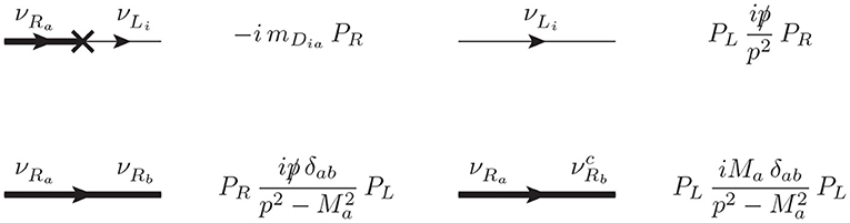
Figure 4. Relevant (dressed) propagators and LFV mass insertion for a general seesaw. All the other Feynman rules needed for the computation of $H\to {\ell }_k{\bar{\ell }}_m$ at one-loop can be found in Arganda et al. [13].

With this setup, the computation is basically the same than that performed in Arganda et al. [13], with the dressed propagator in Equation (22) playing the role of the fat-propagator in Arganda et al. [13]. All the other Feynman rules relevant for the computation of the LFVHD are the same, so we refer to Arganda et al. [13] for further details and conventions.

3.2. The MIA Computation and the Heavy Mass Expansions

We are interested in computing the LFV process $H(p_1)\to {\ell }_k(-p_2){\bar{\ell }}_m(p_3)$, whose decay amplitude can be generically decomposed in terms of two form factors F_L and F_R [9],

$\begin{array}{ll}i{M}=-ig{\overline{u}}_{{\ell }_k}(-p_2)(F_L{P}_L+F_R{P}_R)v_{{\ell }_m}(p_3),& (24)\end{array}$

In order to further simplify our expressions, one could neglect the masses of the charged leptons with respect to the Higgs boson mass. Nevertheless, the form factor F_L(R) is proportional to m_ℓk(m), so we cannot fully neglect lepton masses and we need to keep the leading term. Using the fact that charged lepton masses are hierarchical, we work under the hypothesis m_ℓm ≪ m_ℓk. Then, it is enough to consider the F_L form factor for the $H\to {\ell }_k{\bar{\ell }}_m$ decay, keeping the leading contribution in m_ℓk and neglecting any additional contribution from charged lepton masses³. Then, the partial decay width can be written as:

$\begin{array}{ll}\Gamma (H\to {\ell }_k{\bar{\ell }}_m)=\frac{g^2}{16\pi }{m}_H|F_L{|}^2.& (25)\end{array}$

Equivalently, in this case where m_ℓm ≪ m_ℓk, F_R dominates in the CP-conjugated process $H\to {\ell }_m{\bar{\ell }}_k$. In the Feynman-'t Hooft gauge and in the neutrino mass basis, these form factors receive contributions from the diagrams in Figure 5,

$\begin{array}{ll}{F}_{L,R}={\displaystyle \sum _{\text{i}=1}^{10}}{F}_{L,R}^{(\text{i})}.& (26)\end{array}$

FIGURE 5

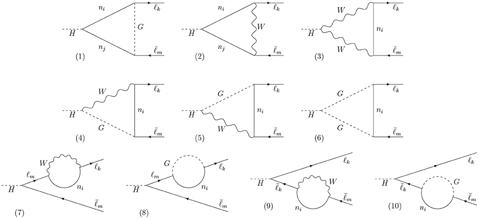
Figure 5. One-loop diagrams in the Feynman-'t Hooft gauge for the process $H\to {\ell }_k{\bar{\ell }}_m$ in the neutrino mass basis.

We remark that the definition of mass basis depends on the perturbation order considered, as loop corrections will generically modified the mass matrix adding non-diagonal terms, which need to be rotated away. We chose to work with the tree-level mass basis and, consequently, we need to include the self-energy corrections to the external legs, last line in Figure 5. Alternatively, one can work with the one-loop level mass basis, which would rotate away those diagrams. Nevertheless, both techniques are equivalent at the one-loop level.

The full analytical expressions for these form factors can be found in Marcano [80]. These expressions are given in terms of the physical neutrino masses and the unitary matrix that relates the flavor and physical basis, so the analytical dependence on the initial parameters in Equation (20) is lost. Morover, evaluating numerically these expression could be time consuming, in particular when the amount of right-handed neutrinos is large. Therefore, it would be useful to have expressions which are given directly in terms of the flavor parameters in Equation (20), even if they are approximations.

As we already know the full result in the physical basis, we could in principle apply the Flavor Expansion Theorem proposed in Dedes et al. [1]. Nevertheless, this technique requires that the external momenta are smaller than the masses running in the loops, and this is not the case in the decay process $H\to {\ell }_k{\bar{\ell }}_m$ due to the fact that the external momentum of the on-shell Higgs is larger than the ν_L and W masses. Therefore, we do not consider this technique for this computation. We perform instead a MIA expansion, since it can be applied even when light masses are running in the loops.

In the MIA, this process can be computed as an expansion of the relevant LFV mass insertions, which in our case are the Dirac mass terms, or equivalently the Yukawa couplings. Thus, each of the diagrams in Figure 5 can be computed in the MIA as,

$\begin{array}{ll}{F}_{L,R}^{\text{MIA\hspace{0.05em}}(\text{i})}=F_{L,R}^{\text{MIA\hspace{0.05em}}(\text{i})}{|}_{Y_{\nu }^2}+F_{L,R}^{\text{MIA\hspace{0.05em}}(\text{i})}{|}_{Y_{\nu }^4}+\dots & (27)\end{array}$

The fact of having only even powers of Y_ν is related to the right-handed neutrinos, whose presence is needed to induce the LFV transition. Since they only interact via the Yukawa couplings, each (dressed) RH propagator will introduce two Y_ν, one at each edge of the propagator. This means that the LO terms ${O}(Y_{\nu }^2)$ will come from MIA diagrams with only one RH propagator, the NLO corrections ${O}(Y_{\nu }^4)$ from diagrams with two, and so on. Being the Yukawa coupling perturbative, it should be enough to compute the first contributions to this expansion. Moreover, the addition of RH propagators will introduce inverse powers of M and ensure the convergence of Equation (27) as a perturbative expansion in terms of ${O}(m_D^2/M^2)$.

We collect the MIA results in Appendix 1, as well as the relevant Feynman diagrams entering the computation. We include the complete ${O}(Y_{\nu }^2)$ terms, which give a good description of the observable when the Yukawa couplings are small. Nevertheless, for large Yukawa couplings, we need to compute also some of the ${O}(Y_{\nu }^4)$ terms [13], which are not as suppressed as we may naively expect from the above discussion. These dominant ${O}(Y_{\nu }^4)$ terms are also given in Appendix 1.

In order to better understand this point, it is useful to analyze our results when the Majorana scale is heavier than the electroweak scale. Indeed, the $O(Y_{\nu }^4)$ terms may become relevant when the Yukawa couplings are large and, since we are working under the hypothesis m_D≪M, it implies heavy Majorana masses. Under this hypothesis of heavy M, the loop integrals contributing to the form factors in Apendix 1 can be expanded in inverse powers of M, as shown in Appendix 2. The obtained result for the form factor can be interpreted as a low-energy effective vertex induced from heavy Majorana neutrinos, $F_L\equiv V_{H{\ell }_k{\bar{\ell }}_m}^{\text{eff}}$.

In this heavy Majorana mass limit, the ${O}(Y_{\nu }^2)$ terms in the MIA expansion contribute dominantly to the order ${O}(m_D^2/M^2)$, as expected. Similarly, we might naively expect that the ${O}(Y_{\nu }^4)$ will contribute as ${O}(m_D^4/M^4)$ and will be, therefore, negligible. Nevertheless, it turns out that some diagrams lead to ${O}(Y_{\nu }^4)$ terms that are suppressed only by two inverse powers of M, and thus they are important to take into account for a good MIA prediction. Indeed, for very large couplings ${O}(Y_{\nu })~1$, these terms may become the dominant ones. In the particular process we are considering, they come from diagrams of type (1), (8), and (10) in Figure 5, whose dominant MIA ${O}(Y_{\nu }^4)$ diagrams are shown in Figure A2.

It is interesting to discuss a bit more the presence of this kind of unsuppressed ${O}(Y_{\nu }^4)$ terms in different LFV observables induced from heavy neutrinos. Besides in the LFV Higgs decays, similar contributions were found in the context of LFV Z boson decays [79], which at the same time suggests that they are also present in LFV 3-body decays, such as ℓ_k → 3ℓ_m, due to the strong correlation between these two latter observables [82, 83]. On the contrary, these terms are not present in the case of LFV radiative decays ℓ_k → ℓ_mγ [10]. The difference could be tracked to the fact that neutrinos do not couple to the photon, but they do couple to the H and Z bosons, leading for example to diagram (1) in Figure 5 for the LFVHD, which is not present in the ℓ_k → ℓ_mγ process⁴. The fact that the radiative decays are different for these other LFV processes is very interesting, as the former are usually the most constraining LFV processes, however this may not be true at very large Yukawa couplings due to these additional terms.

Now, collecting all the relevant terms of ${O}(M^{-2})$, we arrive to the following effective vertex for the LFV $H\to {\ell }_k{\bar{\ell }}_m$ decay,

$\begin{array}{l}{V}_{H{\ell }_k{\overline{\ell }}_m}^{\text{eff}}=\frac{1}{64{\pi }^2}\frac{m_{{\ell }_k}}{m_W}[\frac{m_H^2}{M_a^2}\left(r\left(\frac{m_W^2}{m_H^2}\right)+\log \left(\frac{m_W^2}{M_a^2}\right)\right)\left(Y_{\nu }^{ka}{Y}_{\nu }^{†am}\right)\\ -2v^2{G}(M_a,M_b)\left(Y_{\nu }^{ka}{(Y_{\nu }^{†}{Y}_{\nu })}^{ab}{Y}_{\nu }^{†bm}\right)],& (28)\end{array}$

where we have defined:

$\begin{array}{l}r(\lambda )=-\frac{1}{2}-\lambda -8{\lambda }^2\\ +2(1-2\lambda +8{\lambda }^2)\sqrt{4\lambda -1}\arctan \left(\frac{1}{\sqrt{4\lambda -1}}\right)\\ +16{\lambda }^2(1-2\lambda ){\arctan }^2\left(\frac{1}{\sqrt{4\lambda -1}}\right),\\ {G}(x,y)=\frac{x^2-y^2+(x^2-2y^2)\log \left(\frac{x^2}{y^2}\right)}{{(x^2-y^2)}^2},{G}(x,x)=\frac{3}{2x^2}.& (29)\end{array}$

For the physical values of m_H = 125 GeV and m_W = 80.4 GeV we have $r(m_W^2/m_H^2)~0.31$. We recall again that this expression is valid under the assumption of heavy Majorana masses M ≫ v and in the seesaw limit m_D ≪ M, since we only kept the ${O}(M^{-2})$ terms and we performed the computation at NLO in the MIA expansion. As we will see later, these terms are enough to reproduce the full results to a good accuracy in the parameter space that is still allowed by current constraints.

In Equation (28), we have to sum over the indices a and b, which run over the RH neutrinos. In general, all of them will contribute and the indices will run from 1 to N. Nevertheless, in some interesting cases some of the RH neutrinos might be very heavy and they will completely decouple from the observable. Since the contribution to any very heavy neutrino to Equation (28) is negligible, decoupling a RH neutrino is indeed equivalent to restricting the range of a and b to those (non-decoupled) right-handed neutrinos, which are still light enough to contribute.

Another interesting limit corresponds to the case with complete degenerate RH neutrinos, i.e., M₁ = … = M_N ≡ M. In this case, the effective vertex corresponds to

$\begin{array}{l}{V}_{H{\ell }_k{\overline{\ell }}_m}^{\text{eff}}=\frac{1}{64{\pi }^2}\frac{m_{{\ell }_k}}{m_W}{\displaystyle [\frac{m_H^2}{M^2}\left(r\left(\frac{m_W^2}{m_H^2}\right)+\log \left(\frac{m_W^2}{M^2}\right)\right)Y_{\nu }{Y}_{\nu }^{†}}\\ {\displaystyle -\frac{3v^2}{M^2}{Y}_{\nu }{Y}_{\nu }^{†}{Y}_{\nu }{Y}_{\nu }^{†}{]}^{km}.}& (30)\end{array}$

Notice that, even if have focused on the $H\to {\ell }_k{\bar{\ell }}_m$ channel, the effective vertex $V_{H{\ell }_m{\bar{\ell }}_k}^{\text{eff}}$ of the CP-conjugated process $H\to {\ell }_m{\bar{\ell }}_k$ can be easily obtained by conjugating (Equation 28):

$\begin{array}{ll}{V}_{H{\ell }_m{\bar{\ell }}_k}^{\text{eff}}={\left(V_{H{\ell }_k{\bar{\ell }}_m}^{\text{eff}}\right)}^{*},& (31)\end{array}$

which is equivalent to interchanging the flavor index of the charged leptons k and m in the Yukawa couplings.

Finally, the branching ratio for the process $V_{H{\ell }_k{\bar{\ell }}_m}^{\text{eff}}$ can be computed by just plugging the corresponding effective vertex in Equation (25),

$\begin{array}{ll}\text{BR}(H\to {\ell }_k{\bar{\ell }}_m)=\frac{g^2}{16\pi }\frac{m_H}{{\Gamma }_H^{\text{tot}}}|V_{H{\ell }_k{\bar{\ell }}_m}^{\text{eff}}{|}^2,& (32)\end{array}$

where ${\Gamma }_H^{\text{tot}}$ is the total width of the Higgs boson.

In order to illustrate the accuracy of the effective vertex, we show in Figure 6 the predictions for H → τ$\overline{e}$ computed using the full expressions in the mass basis (solid lines) as well as using the approximated expression in Equation (32). Moreover, we quantify the agreement by means of the ratio R, defined as the approximated prediction over the full one. We choose here a particular realization of the seesaw model that we will introduce in Equation (50), although we found similar results for other examples. The differences between the two panels are the heavy neutrino masses, chosen to be degenerated in the left and hierarchical in the right. The overall conclusion from this figure is that the effective vertex in Equation (28) works very well in both cases, as long as the condition m_D ≪ M is fulfilled.

FIGURE 6

Figure 6. Prediction for BR(H → τ$\overline{e}$) using the exact computation (solid lines) and the effective vertex in Equation (28) (dashed lines). The ratio R = BR_Veff/BR_Full quantifies the agreement between both predictions. The particular seesaw scenario is defined in Equation (50), with Y₀ controlling the global strength of the Yukawa coupling. We consider degenerated heavy neutrinos in the left (M_R2 = M_R1) and hierarchical in the right (M_R2 = 10M_R1).

3.3. Connection to Low Scale Seesaw Models

As a particular but interesting application of the effective vertex in Equation (28), we apply it to the so-called low scale seesaw models (LSS), such as the inverse [85–87] or linear [88] seesaw models. These models are of great phenomenological interest since they can introduce relatively light heavy neutrinos with large Yukawa couplings, and still accommodate naturally the observed light neutrino masses. Moreover, this will also allow us to compare with existing results in the inverse seesaw model [13].

The common feature in all these models is the imposition of an approximate conservation of lepton number [89], which is only violated by some small parameter related to light neutrino masses. The difference between each particular low scale seesaw realization is precisely the nature or origin of this small LNV parameter. However all of them share the same lepton number conserving limit. In our case of study, the LFVHD are LNC processes, and thus the small LNV parameters will not play any important role and we can be neglected. This means that we can expect to have the same LFVHD rates for all these low scale seesaw models.

The LNC low scale seesaws could be realized by adding n_ν pairs of new fermionic singlets with opposite lepton number, which we denote ${\nu }_R^a$ and ${\nu }_S^a$, respectively, with a = 1, …, n_ν. For the purpose of this discussion, we are just interested in the neutrino mass matrix⁵, which in the $({\nu }_L^c,{\nu }_R,{\nu }_S)$ basis reads as

$\begin{array}{ll}{M}_{\text{LSS}}=\left(\begin{array}{ccc}0& v{Y}_{\text{LSS}}& 0\\ v{Y}_{\text{LSS}}^T& 0& M_R\\ 0& M_R^T& 0\end{array}\right),& (33)\end{array}$

where Y_LSS and M_R are, respectively, 3 × n_ν and n_ν × n_ν matrices, and the zeros have the proper dimensions so the total M_LSS matrix is a (3 + 2n_ν) symmetric matrix.

In order to apply our results from the previous Section, the first step is to rotate the heavy neutrino sector to its diagonal form,

$\begin{array}{ll}{U}^T{M}_{\text{LSS }}U=\left(\begin{array}{cc}0& m_D\\ m_D^T& M_{\text{diag}}\end{array}\right)& (34)\end{array}$

where now the dimensions of the new Dirac m_D and Majorana mass M_diag matrices are 3 × 2n_ν and 2n_ν × 2n_ν, respectively, and U is a unitary matrix rotating the neutrino sector. Without any loss of generality, we can assume that M_R is already diagonal and, therefore, the diagonalization becomes trivial,

$\begin{array}{l}U=\left(\begin{array}{cc}{\mathbb{1}}_{{}_3}& 0\\ 0& V\end{array}\right),\\ \text{ with }{M}_{\text{diag}}=V^T\left(\begin{array}{cc}0& M_R\\ M_R& 0\end{array}\right)V=\left(\begin{array}{cc}{M}_R& 0\\ 0& M_R\end{array}\right),& (35)\end{array}$

where the unitary matrix V just contains rotations of π/4 and i factors to make the entries of M_diag possitive. In general, this unitary rotation is defined by four blocks of n_ν × n_ν

$\begin{array}{ll}V=1/\sqrt{2}\left(\begin{array}{cc}{\mathbb{1}}_{n_{\nu }}& -i{\mathbb{1}}_{n_{\nu }}\\ {\mathbb{1}}_{n_{\nu }}& i{\mathbb{1}}_{n_{\nu }}\end{array}\right).& (36)\end{array}$

Finally, the new Dirac mass matrix is given by

$\begin{array}{ll}{m}_D=(v{Y}_{\text{LSS}} 0)V=\frac{v}{\sqrt{2}}(Y_{\text{LSS}}-i{Y}_{\text{LSS}}).& (37)\end{array}$

We have now all the pieces needed to compute the $H\to {\ell }_k{\bar{\ell }}_m$ process, we just need to plug the Dirac matrix m_D = vY_ν of Equation (37) and the M_diag of Equation (35), in the effective vertex of Equation (28). For instance, we can consider the same setup as in Arganda et al. [13], where all the entries of M_R are degenerate. In that case, we can use the Equation (30), with

$\begin{array}{ll}{m}_D{m}_D^{†}=\frac{v^2}{2}(Y_{\text{LSS}}-i{Y}_{\text{LSS}})\left(\begin{array}{c}{Y}_{\text{LSS}}^{†}\\ i{Y}_{\text{LSS}}^{†}\end{array}\right)=v^2{Y}_{\text{LSS}}{Y}_{\text{LSS}}^{†},& (38)\end{array}$

resulting in the effective vertex

$\begin{array}{l}{\displaystyle V_{H{\ell }_k{\overline{\ell }}_m}^{\text{eff}}=\frac{1}{64{\pi }^2}\frac{m_{{\ell }_k}}{m_W}[\frac{m_H^2}{M_R^2}(r\left(\frac{m_W^2}{m_H^2}\right)}\\ {\displaystyle +\log \left(\frac{m_W^2}{M_R^2}\right))Y_{\text{LSS}}{Y}_{\text{LSS}}^{†}-\frac{3v^2}{M_R^2}{Y}_{\text{LSS}}{Y}_{\text{LSS}}^{†}{Y}_{\text{LSS}}{Y}_{\text{LSS}}^{†}{]}^{km},}& (39)\end{array}$

which is agreement with the result in Arganda et al. [13], obtained for the particular case of the inverse seesaw model. Notice that, even that this equation seems to be the same as Equation (30), it is now expressed in terms of the parameters of the low scale seesaw parameters in Equation (33), whose physical interpretation is different from the parameters in Equation (21).

3.4. Numerical Analysis of the LFV Higgs Decays

We conclude this section by applying the derived effective vertex to study how large the LFVHD rates could be in a GSS model after having considered possible constraints from other observables. For that purpose, we will follow the global fit analysis done in Fernandez-Martinez et al. [81], where two different scenarios were considered: a model with only 3 heavy RH neutrinos (3N-SS), and a general seesaw with an arbitrary number of them, as in Equation (20). In both case, the Authors obtained upper bounds on the η matrix, a small Hermitian matrix encoding the deviations from unitarity in the light neutrino mixing. In our case, this matrix can be expressed as⁶,

$\begin{array}{ll}\eta =\frac{1}{2}{m}_D{M}^{-2}{m}_D^{†}=\frac{1}{2}{v}^2{Y}_{\nu }{M}^{-2}{Y}_{\nu }^{†},& (40)\end{array}$

and, at the 2σ level, it is bounded to be below⁷

$\begin{array}{ll}|2{\eta }_{km}|\le {10}^{-3}·\left(\begin{array}{ccc}2.5& 0.024& 2.7\\ 0.024& 0.4& 1.2\\ 2.7& 1.2& 5.6\end{array}\right).& (41)\end{array}$

It is interesting to analyze first the 3N-SS case, as it is simpler. If we assume again the LNC limit, then it can be implemented by

$\begin{array}{ll}{Y}_{\nu }^{\text{3N-SS}}=\left(\begin{array}{ccc}{Y}_e& 0& 0\\ Y_{\mu }& 0& 0\\ Y_{\tau }& 0& 0\end{array}\right),M^{\text{3N-SS}}=\left(\begin{array}{ccc}0& \Lambda & 0\\ \Lambda & 0& 0\\ 0& 0& {\Lambda }^{\prime }\end{array}\right).& (42)\end{array}$

Notice that in this LNC limit light neutrinos are strictly massless, but they can be accommodated by introducing small LNV parameters in these matrices [81]. Nevertheless, since the LFVHD do not violate lepton number, these small LNV parameters will not be relevant for our observable and, therefore, we neglect them in the following.

In this scenario, the effective vertex in Equation (28) becomes,

$\begin{array}{l}{V}_{H{\ell }_k{\overline{\ell }}_m}^{\text{3N-SS}}=\frac{1}{64{\pi }^2}\frac{m_{{\ell }_k}}{m_W}{Y}_k{Y}_m^{*}\{\frac{m_H^2}{{\Lambda }^2}\left(r\left(\frac{m_W^2}{m_H^2}\right)+\log \left(\frac{m_W^2}{{\Lambda }^2}\right)\right)\\ -\frac{3v^2}{{\Lambda }^2}(|Y_e{|}^2+|Y_{\mu }{|}^2+|Y_{\tau }{|}^2)\},& (43)\end{array}$

where we have used that $Y_{\nu }{Y}_{\nu }^{†}{Y}_{\nu }{Y}_{\nu }^{†}=(|Y_e{|}^2+|Y_{\mu }{|}^2+|Y_{\tau }{|}^2)Y_{\nu }{Y}_{\nu }^{†}$. Alternatively, it can be also written in terms of η as,

$\begin{array}{l}{V}_{H{\ell }_k{\overline{\ell }}_m}^{\text{3N-SS}}=\frac{1}{64{\pi }^2}\frac{m_{{\ell }_k}}{m_W}\left(2{\eta }_{km}\right)\{\frac{m_H^2}{v^2}\left(r\left(\frac{m_W^2}{m_H^2}\right)+\log \left(\frac{m_W^2}{{\Lambda }^2}\right)\right)\\ -\frac{3{\Lambda }^2}{v^2}(|2{\eta }_{ee}|+|2{\eta }_{\mu \mu }|+|2{\eta }_{\tau \tau }|)\}.& (44)\end{array}$

Notice that the observable vanishes in the Λ → ∞ limit, as it is manifest in Equation (43). This decoupling behavior is hidden when we express it in terms of η, but this form is useful to conclude on maximum allowed LFVHD rates in this model. Due to the ${O}(Y_{\nu }^4)$ terms, the maximum rates will be obtained at the largest value of Λ that allows to saturate Equation (41) without spoiling the perturbativity of the Yukawa couplings. Assuming a perturbativity bound of $\left|{(Y_{\nu }{Y}_{\nu }^{†})}^{km}\right|<4\pi$, a rough estimation points to Λ ≈ 10 TeV and consequently,

$\begin{array}{ll}\text{BR}(H\to \mu e)\lesssim 10^{-14},& (45)\end{array}$

$\begin{array}{ll}\text{BR}(H\to \tau e)\lesssim 10^{-8},& (46)\end{array}$

$\begin{array}{ll}\text{BR}(H\to \tau \mu )\lesssim 10^{-9},& (47)\end{array}$

where we have defined BR(H → ℓ_kℓ_m) ≡ BR $(H\to {\ell }_k{\bar{\ell }}_m)$ + BR$(H\to {\ell }_m{\bar{\ell }}_k)$. The differences between the three channels have a double origin. From the one side, the fact that these decays are proportional to charged lepton masses suppressed the H → μe with respect to the other two by a factor of $m_{\mu }^2/m_{\tau }^2$. On the other hand, current bounds in Equation (41) are a bit stronger for η_τμ, and much more stringent for η_μe due to the strong constraints coming from μ → eγ [91]. This double suppression makes of H → μe an even more challenging observable for experiments.

The effective vertex in Equation (28) has the advantage of being more general than previously computed ones. In particular, it allows to explore scenarios where the heavy neutrinos have different Majorana masses, as we show in Figure 7. In order not to generate too large masses for light neutrinos, we consider an scenario such as the one in Equation (33), but with only two pairs of Majorana neutrinos (n_ν = 2) contributing to the Higgs decays, assuming that any possible additional neutrino has decoupled from this observable. Moreover, and in order to avoid the strong bounds in the μ-e sector, we have considered a simplified case for the Yukawa couplings where none of the heavy neutrinos couple to muons (left panel) or to electrons (right panel). The rest of the entries of the Yukawa coupling matrix are set to one, again for simplicity. This figure has been done using Equation (28), although we have checked that the full computation leads to the same results in the relevant area allowed by the constraints of Equation (41).

FIGURE 7

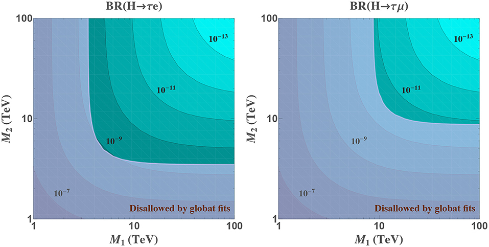
Figure 7. Predictions for LFV Higgs boson decays using Equation (28) in a seesaw model with two pairs of Majorana neutrinos with masses M_R1 and M_R2, as defined in Equation (33). In the left, both neutrinos have Yukawa couplings equal to 1 with electron and tau leptons, and 0 with muons. In the right, we exchange the roles of electrons and muons. Purple shadowed area is disallowed by global fit constraints in Equation (41).

In this Figure 8 we find again the decoupling behavior with each of the individual heavy masses, as we discussed before. We can also see that the predictions for H → τe and H → τμ are the same in both panels, as we have assumed a simplified scenario with equal size Yukawa couplings to the relevant flavors. Nevertheless, the bounds of Equation (41) are stronger in the muon sector than in the electron one, which again implies that the allowed rates are larger for H → τe than for H → τμ. Finally, we notice that the results are symmetric with respect to M_R1 and M_R2, although this is again a consequence of our simplified hypothesis of equal Yukawa couplings, and in general this will not be the case.

FIGURE 8

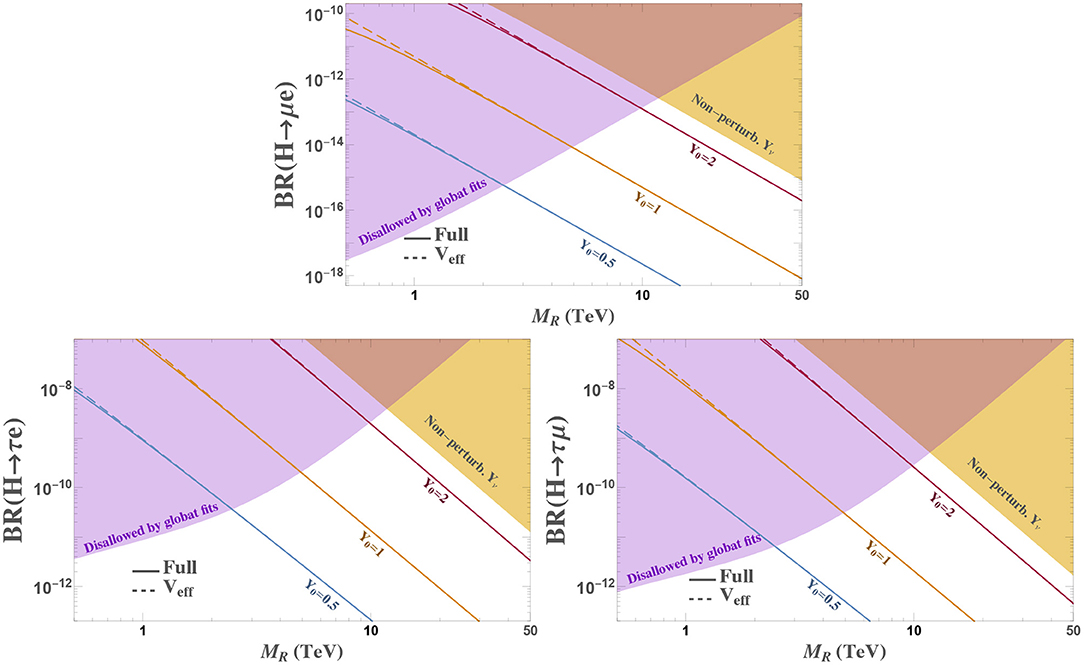
Figure 8. Predictions for the Higgs boson decays into μe (top), τe (left) and τμ (right) computed with the effective vertex in the MIA (dashed lines) and the full results in the physical basis (solid lines) in the context of a low scale seesaw model with Yukawa coupling Y_LSS given by Equation (50). Shadowed areas are disallowed by global fits constraints (purple) and the non-perturbative regime for the Yukawa couplings (yellow), which we define as $\left|{(Y_{\nu }{Y}_{\nu }^{†})}^{km}\right|>4\pi$ for any element.

In a more general scenario, the η matrix will constrain a combination of all the heavy neutrino mixing to the active state, each of these contributions being of order ${\xi }_{\ell a}=m_D^{\ell a}/M_a$, where $\xi =m_D{M}^{-1}$ is the usual seesaw parameter. Generalizing the description of Arganda et al. [13] to the case of having N RH neutrinos, we can think of this parameter as made of three N-vectors:

$\begin{array}{ll}\xi =\left(\begin{array}{c}{\xi }_e\\ {\xi }_{\mu }\\ {\xi }_{\tau }\end{array}\right)=\left(\begin{array}{cccc}{\xi }_{e1}& {\xi }_{e2}& \cdots & {\xi }_{eN}\\ {\xi }_{\mu 1}& {\xi }_{\mu 2}& \cdots & {\xi }_{\mu N}\\ {\xi }_{\tau 1}& {\xi }_{\tau 2}& \cdots & {\xi }_{\tau N}\end{array}\right),& (48)\end{array}$

which leads to

$\begin{array}{ll}2\eta =\xi {\xi }^{†}=\left(\begin{array}{ccc}|{\xi }_e{|}^2& {\xi }_e·{\xi }_{\mu }^{*}& {\xi }_e·{\xi }_{\tau }^{*}\\ {\xi }_{\mu }·{\xi }_e^{*}& |{\xi }_{\mu }{|}^2& {\xi }_{\mu }·{\xi }_{\tau }^{*}\\ {\xi }_{\tau }·{\xi }_e^{*}& {\xi }_{\tau }·{\xi }_{\mu }^{*}& |{\xi }_{\tau }{|}^2\end{array}\right).& (49)\end{array}$

This implies that the diagonal entries of the η matrix constrain the modulus of these N-vectors, while the diagonal ones set upper bounds on the complex scalar products between them. Moreover, this geometrical picture is also useful to find solutions that accommodate the current bounds given in Equation (41), as we only need to set the modulus and angles between these vectors, and to explore the implications on our LFV observable.

Let us consider a final example to illustrate this latter point. In order to avoid issues generating too large contributions to light neutrino masses, an elegant solution is to consider a low scale seesaw realization of the model, as we introduced in Equation (33). If we assume, for example, that there are two pairs of sterile fermions (n_ν = 2) contributing to our observable and that they have the same mass, M_R1 = M_R2 ≡ M_R, an interesting value for the Yukawa matrix is the following:

$\begin{array}{ll}{Y}_{\text{LSS}}=Y_0\left(\begin{array}{cc}1& 0\\ 0.008& 0.42\\ 1& 1.1\end{array}\right).& (50)\end{array}$

This example is useful as it leads to a η matrix with a very similar pattern than that in Equation (41). Then, depending on the value of the global strength factor Y₀ and the mass M_R, we can define which part of the parameter space is allowed.

We show in Figure 8 the predictions for the three LFVHD channels in this particular example, although we expect similar results for other models with more RH neutrinos as long as they lead to the similar η matrices. The first thing we see from this figure is that the effective vertex (dashed lines) matches very well the full prediction (solid lines), as we already saw before. Nevertheless, the simple expression of Equation (28) allows us to easily understand the dependence on the different parameters of the model. Finally, we can also use this figure to deduce how large LFVHD rates can we expect after having considered the bounds in Equation (41) as well as perturbativity bounds. As we discussed above, the largest possible values are obtained for heavy masses at around 10 TeV, when the bounds from the global fit analysis and perturbativity cross. Unfortunately, the branching ratios in the allowed white area are too small and far from current experimental sensitivities.

4. Conclusions

In this work, we have discussed the importance of having expressions for lepton flavor violating transitions which are expressed directly in terms of the fundamental parameters of the model. These expressions are helpful to better understand the observable, as well as to compare it with experimental observations in order to constrain the interaction parameter space. In this context, the mass insertion approximation technique is a powerful tool, which we have reviewed with two simple examples.

We have then studied the LFV Higgs decays in the context of a general type-I seesaw model with an arbitrary number of right-handed neutrinos. We applied the MIA technique to this model, which allowed us to derived an effective vertex for Hℓ_kℓ_m after integrating out the heavy right-handed neutrinos. This analytical expression is useful to understand the behavior of the observables with the fundamental parameters of the neutrino sector, i.e., the Yukawa couplings and the heavy Majorana masses. Moreover, it also provides an alternative way to quickly evaluate these observables to a very good approximation, without the need of long numerical evaluations of the full result in the physical basis.

Finally, we have made the connection to the phenomenologically interesting case of low scale seesaw models. After explicitly checking that we recover existing results for the inverse seesaw case, we have evaluated the LFVHD rates taking into account current bounds from global analysis, as well as perturbativity bounds for the Yukawa couplings. Unfortunately, the predicted rates for the LFVHD in the allowed area are far from current experimental sensitivities and, consequently, they do not provide a competitive way of probing the existence of these heavy Majorana neutrinos.

Data Availability Statement

The datasets generated for this study are available on request to the corresponding author.

Author Contributions

All authors listed have made a substantial, direct and intellectual contribution to the work, and approved it for publication.

Funding

This work was supported by the European Union through the ITN ELUSIVES H2020-MSCA-ITN-2015//674896 and the RISE INVISIBLESPLUS H2020-MSCA-RISE-2015//690575, by the CICYT through the project FPA2016-78645-P, and by the Spanish MINECO's Centro de Excelencia Severo Ochoa Programme under grant SEV-2016-0597.

Conflict of Interest

The authors declare that the research was conducted in the absence of any commercial or financial relationships that could be construed as a potential conflict of interest.

Acknowledgments

We would like to thank Claudia García-García for a careful reading of the manuscript.

Supplementary Material

The Supplementary Material for this article can be found online at: https://www.frontiersin.org/articles/10.3389/fphy.2019.00228/full#supplementary-material

Footnotes

1. ^Notice that, in these references, particular realizations of the type-I seesaw model were considered. Nevertheless, since the expressions are given in the physical basis, the generalization to a GSS is trivially obtained by just changing the range of neutrino indices.

2. ^A full computation in a general R_ξ gauge and proof of gauge invariance can be found in Arganda et al. [13].

3. ^For complete results, we refer to Arganda et al. [13] and Marcano [80].

4. ^In the neutrino mass basis, this can be understood as the additional contribution due to the neutrino neutral current, as discussed in e.g., Pilaftsis et al. [7] and Abada et al. [84].

5. ^For more details on LSS, see for instance [90].

6. ^Notice that our definition of Y_ν corresponds to $Y_{\nu }^{†}$ in Fernandez-Martinez et al. [81].

7. ^These bounds correspond actually to the GSS, although very similar bounds are obtained for the 3N-SS scenario.

References

1. Dedes A, Paraskevas M, Rosiek J, Suxho K, Tamvakis K. Mass insertions vs. mass eigenstates calculations in flavour physics. J High Energy Phys. (2015) 6:151. doi: 10.1007/JHEP06(2015)151

CrossRef Full Text | Google Scholar

2. Rosiek J. MassToMI a mathematica package for an automatic mass insertion expansion. Comput Phys Commun. (2016) 201:144–58. doi: 10.1016/j.cpc.2015.12.011

CrossRef Full Text | Google Scholar

3. CMS Collaboration. Search for lepton flavour violating decays of the Higgs boson to eτ and eμ in protonproton collisions at $\sqrt{s}=$ 8 TeV. Phys Lett B. (2016) 763:472–500. doi: 10.1016/j.physletb.2016.09.062

CrossRef Full Text | Google Scholar

4. ATLAS Collaboration. Searches for lepton-flavour-violating decays of the Higgs boson in $\sqrt{s}=13$ TeV pp collisions with the ATLAS detector. Phys. Lett. B. (2020) 800:135069. doi: 10.1016/j.physletb.2019.135069

CrossRef Full Text | Google Scholar

5. CMS Collaboration. Search for lepton flavour violating decays of the Higgs boson to μτ and eτ in proton-proton collisions at $\sqrt{s}=$ 13 TeV. J High Energy Phys. (2018) 6:1. doi: 10.1007/JHEP06(2018)001

CrossRef Full Text | Google Scholar

6. Aaij R, Beteta CA, Adeva B, Adinolfi M, Aidala CA, Ajaltouni Z, et al. Search for lepton-flavour-violating decays of Higgs-like bosons. Eur Phys J C. (2018) 78:1008. doi: 10.1140/epjc/s10052-018-6386-8

PubMed Abstract | CrossRef Full Text | Google Scholar

7. Pilaftsis A. Lepton flavor nonconservation in H0 decays. Phys Lett B. (1992) 285:68–74. doi: 10.1016/0370-2693(92)91301-O

CrossRef Full Text | Google Scholar

8. Korner JG, Pilaftsis A, Schilcher K. Leptonic CP asymmetries in flavor changing H0 decays. Phys Rev D. (1993) 47:1080–6. doi: 10.1103/PhysRevD.47.1080

PubMed Abstract | CrossRef Full Text | Google Scholar

9. Arganda E, Curiel AM, Herrero MJ, Temes D. Lepton flavor violating Higgs boson decays from massive seesaw neutrinos. Phys Rev D. (2005) 71:035011. doi: 10.1103/PhysRevD.71.035011

CrossRef Full Text | Google Scholar

10. Arganda E, Herrero MJ, Marcano X, Weiland C. Imprints of massive inverse seesaw model neutrinos in lepton flavor violating Higgs boson decays. Phys Rev D. (2015) 91:015001. doi: 10.1103/PhysRevD.91.015001

CrossRef Full Text | Google Scholar

11. Arganda E, Herrero MJ, Marcano X, Weiland C. Enhancement of the lepton flavor violating Higgs boson decay rates from SUSY loops in the inverse seesaw model. Phys Rev D. (2016) 93:055010. doi: 10.1103/PhysRevD.93.055010

CrossRef Full Text | Google Scholar

12. Aoki M, Kanemura S, Sakurai K, Sugiyama H. Testing neutrino mass generation mechanisms from the lepton flavor violating decay of the Higgs boson. Phys Lett B. (2016) 763:352–7. doi: 10.1016/j.physletb.2016.10.055

CrossRef Full Text | Google Scholar

13. Arganda E, Herrero MJ, Marcano X, Morales R, Szynkman A. Effective lepton flavor violating Hij vertex from right-handed neutrinos within the mass insertion approximation. Phys Rev D. (2017) 95:095029. doi: 10.1103/PhysRevD.95.095029

CrossRef Full Text | Google Scholar

14. Herrero-García J, Ohlsson T, Riad S, Wirn J. Full parameter scan of the Zee model: exploring Higgs lepton flavor violation. J High Energy Phys. (2017) 4:130. doi: 10.1007/JHEP04(2017)130

CrossRef Full Text | Google Scholar

15. Thao NH, Hue LT, Hung HT, Xuan NT. Lepton flavor violating Higgs boson decays in seesaw models: new discussions. Nucl Phys B. (2017) 921:159–80. doi: 10.1016/j.nuclphysb.2017.05.014

CrossRef Full Text | Google Scholar

16. Dery A, Efrati A, Hiller G, Hochberg Y, Nir Y. Higgs couplings to fermions: 2HDM with MFV. J High Energy Phys (2013) 8:6. doi: 10.1007/JHEP08(2013)006

CrossRef Full Text | Google Scholar

17. Dery A, Efrati A, Nir Y, Soreq Y, SusiÄ V. Model building for flavor changing Higgs couplings. Phys Rev D. (2014) 90:115022. doi: 10.1103/PhysRevD.90.115022

CrossRef Full Text | Google Scholar

18. He XG, Tandean J, Zheng YJ. Higgs decay h with minimal flavor violation. J High Energy Phys. (2015) 9:93. doi: 10.1007/JHEP09(2015)093

CrossRef Full Text | Google Scholar

19. Baek S, Tandean J. Flavor-changing Higgs decays in grand unification with minimal flavor violation. Eur Phys J C. (2016) 76:673. doi: 10.1140/epjc/s10052-016-4486-x

CrossRef Full Text | Google Scholar

20. Han T, Marfatia D. h–> μτ at hadron colliders. Phys Rev Lett. (2001) 86:1442–5. doi: 10.1103/PhysRevLett.86.1442

PubMed Abstract | CrossRef Full Text | Google Scholar

21. Curiel AM, Herrero MJ, Temes D. Flavor changing neutral Higgs boson decays from squark Gluino loops. Phys Rev D. (2003) 67:075008. doi: 10.1103/PhysRevD.67.075008

CrossRef Full Text | Google Scholar

22. Diaz-Cruz JL. A More flavored Higgs boson in supersymmetric models. J High Energy Phys. (2003) 5:36. doi: 10.1088/1126-6708/2003/05/036

CrossRef Full Text | Google Scholar

23. Curiel AM, Herrero MJ, Hollik W, Merz F, Penaranda S. SUSY electroweak one loop contributions to flavor changing Higgs-Boson decays. Phys Rev D. (2004) 69:075009. doi: 10.1103/PhysRevD.69.075009

CrossRef Full Text | Google Scholar

24. Brignole A, Rossi A. Lepton flavor violating decays of supersymmetric Higgs bosons. Phys Lett B. (2003) 566:217–25. doi: 10.1016/S0370-2693(03)00837-2

CrossRef Full Text | Google Scholar

25. Brignole A, Rossi A. Anatomy and phenomenology of mu-tau lepton flavor violation in the MSSM. Nucl Phys B. (2004) 701:3–53. doi: 10.1016/j.nuclphysb.2004.08.037

CrossRef Full Text | Google Scholar

26. Parry JK. Lepton flavor violating Higgs boson decays, τ → μγ and $B_s\to {\mu }^{+}{\mu }^{-}$ in the constrained MSSM+NR with large tan beta. Nucl Phys B. (2007) 760:38–63. doi: 10.1016/j.nuclphysb.2006.10.011

CrossRef Full Text | Google Scholar

27. Diaz-Cruz JL, Ghosh DK, Moretti S. Lepton flavour violating heavy Higgs decays within the νMSSM and their detection at the LHC. Phys Lett B. (2009) 679:376–81. doi: 10.1016/j.physletb.2009.07.065

CrossRef Full Text | Google Scholar

28. Crivellin A. Effective Higgs vertices in the generic MSSM. Phys Rev D. (2011) 83:056001. doi: 10.1103/PhysRevD.83.056001

CrossRef Full Text | Google Scholar

29. Giang PT, Hue LT, Huong DT, Long HN. Lepton-flavor violating decays of neutral higgs to muon and tauon in supersymmetric economical 3-3-1 model. Nucl Phys B. (2012) 864:85–112. doi: 10.1016/j.nuclphysb.2012.06.008

CrossRef Full Text | Google Scholar

30. Arhrib A, Cheng Y, Kong OCW. Higgs to mu+tau decay in supersymmetry without R-parity. EPL. (2013) 101:31003. doi: 10.1209/0295-5075/101/31003

CrossRef Full Text | Google Scholar

31. Arhrib A, Cheng Y, Kong OCW. Comprehensive analysis on lepton flavor violating Higgs boson to μ^∓τ^± decay in supersymmetry without R parity. Phys Rev D. (2013) 87:015025. doi: 10.1103/PhysRevD.87.015025

CrossRef Full Text | Google Scholar

32. Arana-Catania M, Arganda E, Herrero MJ. Non-decoupling SUSY in LFV Higgs decays: a window to new physics at the LHC. J High Energy Phys. (2013) 9:160. [Erratum: J High Energy Phys. 10:192(2015)]. doi: 10.1007/JHEP10(2015)192

CrossRef Full Text | Google Scholar

33. Arganda E, Herrero MJ, Morales R, Szynkman A. Analysis of the h, H, A decays induced from SUSY loops within the Mass Insertion approximation. J High Energy Phys. (2016) 3:55. doi: 10.1007/JHEP03(2016)055

CrossRef Full Text | Google Scholar

34. Aloni D, Nir Y, Stamou E. Large BR(h → τμ) in the MSSM? J High Energy Phys. (2016) 4:162. doi: 10.1007/JHEP04(2016)162

CrossRef Full Text | Google Scholar

35. Vicente A. Lepton flavor violation beyond the MSSM. Adv High Energy Phys. (2015) 2015:686572. doi: 10.1155/2015/686572

CrossRef Full Text | Google Scholar

36. Alvarado C, Capdevilla RM, Delgado A, Martin A. Minimal models of loop-induced lepton flavor violation in Higgs boson decays. Phys Rev D. (2016) 94:075010. doi: 10.1103/PhysRevD.94.075010

CrossRef Full Text | Google Scholar

37. Hammad A, Khalil S, Un CS. Large BR(h → τμ) in supersymmetric models. Phys Rev D. (2017) 95:055028. doi: 10.1103/PhysRevD.95.055028

CrossRef Full Text | Google Scholar

38. Gomez ME, Heinemeyer S, Rehman M. Lepton flavor violating Higgs Boson Decays in Supersymmetric High Scale Seesaw Models 2017). arXiv:1703.02229. doi: 10.22606/jpp.2017.11003

CrossRef Full Text | Google Scholar

39. Davidson S, Grenier GJ. Lepton flavour violating Higgs and tau to mu gamma. Phys Rev D. (2010) 81:095016. doi: 10.1103/PhysRevD.81.095016

CrossRef Full Text

40. Aristizabal Sierra D, Vicente A. Explaining the CMS Higgs flavor violating decay excess. Phys Rev D. (2014) 90:115004. doi: 10.1103/PhysRevD.90.115004

CrossRef Full Text | Google Scholar

41. Omura Y, Senaha E, Tobe K. Lepton-flavor-violating Higgs decay h → μτ and muon anomalous magnetic moment in a general two Higgs doublet model. J High Energy Phys. (2015) 5:28. doi: 10.1007/JHEP05(2015)028

CrossRef Full Text | Google Scholar

42. Bizot N, Davidson S, Frigerio M, Kneur JL. Two Higgs doublets to explain the excesses pp → γγ(750 GeV) and h → τ^±μ^∓. J High Energy Phys. (2016) 3:73. doi: 10.1007/JHEP03(2016)073

CrossRef Full Text | Google Scholar

43. Botella FJ, Branco GC, Nebot M, Rebelo MN. Flavour changing Higgs couplings in a class of two Higgs doublet models. Eur Phys J C. (2016) 76:161. doi: 10.1140/epjc/s10052-016-3993-0

CrossRef Full Text | Google Scholar

44. Agashe K, Contino R. Composite Higgs-mediated FCNC. Phys Rev D. (2009) 80:075016. doi: 10.1103/PhysRevD.80.075016

CrossRef Full Text

45. Perez G, Randall L. Natural neutrino masses and mixings from warped geometry. J High Energy Phys. (2009) 1:77. doi: 10.1088/1126-6708/2009/01/077

CrossRef Full Text | Google Scholar

46. Casagrande S, Goertz F, Haisch U, Neubert M, Pfoh T. Flavor physics in the Randall-Sundrum model: I. Theoretical setup and electroweak precision tests. J High Energy Phys. (2008) 10:94. doi: 10.1088/1126-6708/2008/10/094

CrossRef Full Text | Google Scholar

47. Albrecht ME, Blanke M, Buras AJ, Duling B, Gemmler K. Electroweak and flavour structure of a warped extra dimension with custodial protection. J High Energy Phys. (2009) 9:64. doi: 10.1088/1126-6708/2009/09/064

CrossRef Full Text | Google Scholar

48. Azatov A, Toharia M, Zhu L. Higgs mediated FCNC's in warped extra dimensions. Phys Rev D. (2009) 80:035016. doi: 10.1103/PhysRevD.80.035016

CrossRef Full Text

49. Diaz-Cruz JL, Toscano JJ. Lepton flavor violating decays of Higgs bosons beyond the standard model. Phys Rev D. (2000) 62:116005. doi: 10.1103/PhysRevD.62.116005

CrossRef Full Text | Google Scholar

50. de Lima L, Machado CS, Matheus RD, do Prado LAF. Higgs flavor violation as a signal to discriminate models. J High Energy Phys. (2015) 11:74. doi: 10.1007/JHEP11(2015)074

CrossRef Full Text | Google Scholar

51. Buschmann M, Kopp J, Liu J, Wang XP. New signatures of flavor violating Higgs couplings. J High Energy Phys. (2016) 6:149. doi: 10.1007/JHEP06(2016)149

CrossRef Full Text | Google Scholar

52. Herrero-Garcia J, Rius N, Santamaria A. Higgs lepton flavour violation: UV completions and connection to neutrino masses. J High Energy Phys. (2016) 11:84. doi: 10.1007/JHEP11(2016)084

CrossRef Full Text | Google Scholar

53. Blusca-Mato H, Falkowski A. On the exotic Higgs decays in effective field theory. Eur Phys J C. (2016) 76:514. doi: 10.1140/epjc/s10052-016-4362-8

CrossRef Full Text | Google Scholar

54. Coy R, Frigerio M. Effective approach to lepton observables: the seesaw case. Phys Rev D. (2019) 99:095040. doi: 10.1103/PhysRevD.99.095040

CrossRef Full Text | Google Scholar

55. Blankenburg G, Ellis J, Isidori G. Flavour-changing decays of a 125 GeV Higgs-like particle. Phys Lett B. (2012) 712:386–90. doi: 10.1016/j.physletb.2012.05.007

CrossRef Full Text | Google Scholar

56. Harnik R, Kopp J, Zupan J. Flavor violating Higgs decays. J High Energy Phys. (2013) 3:26. doi: 10.1007/JHEP03(2013)026

CrossRef Full Text | Google Scholar

57. Dery A, Efrati A, Hochberg Y, Nir Y. What if BR(h → μμ) $BR(h\to \tau \tau )\ne m_{\mu }^2/m_{\tau }^2$? J High Energy Phys. (2013) 5:39. doi: 10.1007/JHEP05(2013)039

CrossRef Full Text

58. Falkowski A, Straub DM, Vicente A. Vector-like leptons: Higgs decays and collider phenomenology. J High Energy Phys. (2014) 5:92. doi: 10.1007/JHEP05(2014)092

CrossRef Full Text | Google Scholar

59. Campos MD, Cárcamo Hernández AE, Päs H, Schumacher E. Higgs → μτ as an indication for S₄ flavor symmetry. Phys Rev D. (2015) 91:116011. doi: 10.1103/PhysRevD.91.116011

CrossRef Full Text | Google Scholar

60. Heeck J, Holthausen M, Rodejohann W, Shimizu Y. Higgs in Abelian and non-Abelian flavor symmetry models. Nucl Phys B. (2015) 896:281–310. doi: 10.1016/j.nuclphysb.2015.04.025

CrossRef Full Text | Google Scholar

61. Crivellin A, D'Ambrosio G, Heeck J. Explaining h → μ^±τ^∓, B→K^*μ⁺μ⁻ and B→Kμ⁺μ⁻/B→Ke⁺e⁻ in a two-Higgs-doublet model with gauged L_μ−L_τ. Phys Rev Lett. (2015) 114:151801. doi: 10.1103/PhysRevLett.114.151801

CrossRef Full Text | Google Scholar

62. Dorner I, Fajfer S, Greljo A, Kamenik JF, Konik N, Niandic I. New physics models facing lepton flavor violating Higgs decays at the percent level. J High Energy Phys. (2015) 6:108. doi: 10.1007/JHEP06(2015)108

CrossRef Full Text | Google Scholar

63. Baek S, Kang ZF. Naturally large radiative lepton flavor violating Higgs decay mediated by lepton-flavored dark matter. J High Energy Phys. (2016) 3:106. doi: 10.1007/JHEP03(2016)106

CrossRef Full Text | Google Scholar

64. Huitu K, Keus V, Koivunen N, Lebedev O. Higgs-flavon mixing and h → μτ. J High Energy Phys. (2016) 5:26. doi: 10.1007/JHEP05(2016)026

CrossRef Full Text | Google Scholar

65. Baek S, Nomura T, Okada H. An explanation of one-loop induced h decay. Phys Lett B. (2016) 759:91–8. doi: 10.1016/j.physletb.2016.05.055

CrossRef Full Text | Google Scholar

66. Altmannshofer W, Carena M, Crivellin A. L_μ−L_τ theory of Higgs flavor violation and (g−2)_μ. Phys Rev D. (2016) 94:095026. doi: 10.1103/PhysRevD.94.095026

CrossRef Full Text | Google Scholar

67. Di Iura A, Herrero-Garcia J, Meloni D. Phenomenology of SU(5) low-energy realizations: the diphoton excess and Higgs flavor violation. Nucl Phys B. (2016) 911:388–424. doi: 10.1016/j.nuclphysb.2016.08.005

CrossRef Full Text | Google Scholar

68. Nguyen TP, Le TT, Hong TT, Hue LT. Decay of standard model-like Higgs boson h → μτ in a 3-3-1 model with inverse seesaw neutrino masses. Phys Rev D. (2018) 97:073003. doi: 10.1103/PhysRevD.97.073003

CrossRef Full Text | Google Scholar

69. Minkowski P. μ → eγ at a Rate of One Out of 10⁹ Muon Decays? Phys Lett B. (1977) 67:421–8. doi: 10.1016/0370-2693(77)90435-X

CrossRef Full Text | Google Scholar

70. Gell-Mann M, Ramond P, Slansky R. Complex spinors and unified theories. Conf Proc C. (1979) 790927:315–21.

Google Scholar

71. Yanagida T. Horizontal gauge symmetry and masses of neutrinos. Conf Proc C. (1979) 7902131:95–9.

Google Scholar

72. Mohapatra RN, Senjanovic G. Neutrino mass and spontaneous parity nonconservation. Phys Rev Lett. (1980) 44:912. doi: 10.1103/PhysRevLett.44.912

CrossRef Full Text | Google Scholar

73. Schechter J, Valle JWF. Neutrino masses in SU(2) x U(1) theories. Phys Rev D. (1980) 22:2227. doi: 10.1103/PhysRevD.22.2227

CrossRef Full Text | Google Scholar

74. Super-Kamiokande Collaboration. Evidence for oscillation of atmospheric neutrinos. Phys Rev Lett. (1998) 81:1562–7. doi: 10.1103/PhysRevLett.81.1562

CrossRef Full Text | Google Scholar

75. Super-Kamiokande Collaboration. Measurement of the flux and zenith-angle distribution of upward through going muons by Super-Kamiokande. Phys Rev Lett. (1999) 82:2644–8. doi: 10.1103/PhysRevLett.82.2644

CrossRef Full Text | Google Scholar

76. SNO Collaboration. Direct evidence for neutrino flavor transformation from neutral current interactions in the Sudbury Neutrino Observatory. Phys Rev Lett. (2002) 89:011301. doi: 10.1103/PhysRevLett.89.011301

CrossRef Full Text | Google Scholar

77. KamLAND Collaboration. First results from KamLAND: evidence for reactor anti-neutrino disappearance. Phys Rev Lett. (2003) 90:021802. doi: 10.1103/PhysRevLett.90.021802

CrossRef Full Text | Google Scholar

78. Abada A, Teixeira AM. Heavy neutral leptons and high-intensity observables. Front Phys. (2018) 6:142. doi: 10.3389/fphy.2018.00142

CrossRef Full Text | Google Scholar

79. Herrero MJ, Marcano X, Morales R, Szynkman A. One-loop effective LFV Zl_kl_m vertex from heavy neutrinos within the mass insertion approximation. Eur Phys J C. (2018) 78:815. doi: 10.1140/epjc/s10052-018-6281-3

CrossRef Full Text | Google Scholar

80. Marcano X. Lepton Flavor Violation From Low Scale Seesaw Neutrinos With Masses Reachable at the LHC. UAM (2017). arXiv:1710.08032. doi: 10.1007/978-3-319-94604-7

CrossRef Full Text | Google Scholar

81. Fernandez-Martinez E, Hernandez-Garcia J, Lopez-Pavon J. Global constraints on heavy neutrino mixing. J High Energy Phys. (2016) 8:33. doi: 10.1007/JHEP08(2016)033

CrossRef Full Text | Google Scholar

82. Abada A, De Romeri V, Monteil S, Orloff J, Teixeira AM. Indirect searches for sterile neutrinos at a high-luminosity Z-factory. J High Energy Phys. (2015) 4:51. doi: 10.1007/JHEP04(2015)051

CrossRef Full Text | Google Scholar

83. De Romeri V, Herrero MJ, Marcano X, Scarcella F. Lepton flavor violating Z decays: a promising window to low scale seesaw neutrinos. Phys Rev D. (2017) 95:075028. doi: 10.1103/PhysRevD.95.075028

CrossRef Full Text | Google Scholar

84. Abada A, Beirevi D, Lucente M, Sumensari O. Lepton flavor violating decays of vector quarkonia and of the Z boson. Phys Rev D. (2015) 91:113013. doi: 10.1103/PhysRevD.91.113013

CrossRef Full Text | Google Scholar

85. Mohapatra RN. Mechanism for understanding small neutrino mass in superstring theories. Phys Rev Lett. (1986) 56:561–3. doi: 10.1103/PhysRevLett.56.561

PubMed Abstract | CrossRef Full Text | Google Scholar

86. Mohapatra RN, Valle JWF. Neutrino mass and baryon number nonconservation in superstring models. Phys Rev D. (1986) 34:1642. doi: 10.1103/PhysRevD.34.1642

PubMed Abstract | CrossRef Full Text | Google Scholar

87. Bernabeu J, Santamaria A, Vidal J, Mendez A, Valle JWF. Lepton flavor nonconservation at high-energies in a superstring inspired standard model. Phys Lett B. (1987) 187:303–8. doi: 10.1016/0370-2693(87)91100-2

CrossRef Full Text | Google Scholar

88. Malinsky M, Romao JC, Valle JWF. Novel supersymmetric SO(10) seesaw mechanism. Phys Rev Lett. (2005) 95:161801. doi: 10.1103/PhysRevLett.95.161801

CrossRef Full Text | Google Scholar

89. Moffat K, Pascoli S, Weiland C. Equivalence between massless neutrinos and lepton number conservation in fermionic singlet extensions of the Standard Model (2017). arXiv:1712.07611.

Google Scholar

90. Weiland C. Effects of Fermionic Singlet Neutrinos on High- and Low-Energy Observables. Orsay: LPT (2013). arXiv:1311.5860.

Google Scholar

91. MEG Collaboration. Search for the lepton flavour violating decay μ⁺→e⁺γ with the full dataset of the MEG experiment. Eur Phys J C. (2016) 76:434. doi: 10.1140/epjc/s10052-016-4271-x

CrossRef Full Text | Google Scholar

92. Passarino G, Veltman MJG. One loop corrections for e+e- annihilation into μ+μ- in the weinberg model. Nucl Phys B. (1979) 160:151–207. doi: 10.1016/0550-3213(79)90234-7

CrossRef Full Text | Google Scholar

93. Hahn T, Perez-Victoria M. Automatized one loop calculations in four-dimensions and D-dimensions. Comput Phys Commun. (1999) 118:153–65. doi: 10.1016/S0010-4655(98)00173-8

CrossRef Full Text | Google Scholar