A Three-Dimensional Numerical Model of an Active Cell Cortex in the Viscous Limit

1 Introduction

Motor proteins in living cells are capable of converting chemically stored energy into movement and mechanical work [1] and therefore drive biophysical systems out of thermodynamic equilibrium [2]. Such motor proteins actively induce stresses [2–5], which lead to the formation of patterns [6–9] or spontaneous flows [10–18]. In the cell cortex, which is a network of cytoskeletal actin filaments and myosin proteins [1] enclosing the cell interior, such an active material is confined to a thin layer. Together with the plasma membrane the cell cortex can strongly deform and therefore plays a crucial role in the regulation of the cell shape [19–23] and movement [24–29]. A prominent example is the cytokinesis in cell division, where a ring of cortical actomyosin leads to furrow constriction and in turn to the separation of the two daughter cells [30–34].

Materials containing cytoskeletal filaments and motor proteins are successfully described by active gel theory [2, 35–37]. Its key ingredient is the actively induced force by the motor proteins, which leads to an active stress in the material [38, 39]. In addition, polymerization and depolymerization lead to transient changes within the active gel [20, 35]. Focusing on the cell cortex of actomyosin or on epithelial tissue, active gel theory has recently been formulated in the framework of thin shell theory [40]. The generic active gel theory [35] incorporates the viscoelastic nature of the cytoskeletal assemblies, where the presence of an active stress triggers both elastic deformations and viscous flows. Starting from the viscoelastic theory two limits of the cortex behavior can be considered, the elastic limit [40–43] and the viscous limit [21, 28, 30, 33, 40, 44, 45]. In the latter, viscous flows arise which are responsible for a large number of cellular processes. In cell morphogenesis transitions from a spherical initial shape to pear-like [20, 21] or oblate [8] shapes have been reported. Cell division has successfully been modeled [30, 31, 33, 34, 44, 46] including a threshold active stress needed to complete cytokinesis [33]. Further examples include cell movement [24, 47] and embryogenesis [19, 48, 49].

Such investigations involving the cell cortex are based on either analytical calculations [21, 30, 41, 44] or numerical simulations [9, 33, 42, 45, 47, 50, 51]. Farutin et al. [47] investigated cell crawling by coupling cortical mechanics to the boundary integral equation in an axisymmetric treatment. Turlier et al. [33] used a numerical, axisymmetric formulation of cell cytokinesis advecting tracer points to track the position of the membrane. Mietke et al. [9] developed another axisymmetric simulation method by discretizing the arc length of the cellular membrane. Including myosin activity in terms of a preferred curvature in the framework of an elastic shell, Heer et al. [50] determined the equilibrium of a tissue shell in three dimensions. Torres-Sánchez et al. [45] developed a fully three-dimensional computational model of a viscous active cell cortex in the absence of an external fluid. Being based on Onsager’s variational principle [52] their method utilizes a subdivision finite element scheme for discretization. A generalization of the latter to arbitrary topology using local Monge parametrization method has been provided [51]. Recently, two of us have developed a dynamic three-dimensional simulation model of an active cell cortex in the elastic limit based on a parabolic fitting procedure [42]. This approach provides the advantage that it is dynamically coupled to the surrounding fluid flow using the lattice-Boltzmann/immersed boundary method and thus allows one to study cortical dynamics in realistic environments such as, e.g., blood flow [43].

In the present manuscript we develop a new method, transferring the ideas of ref. [42] to the viscous limit in order to numerically obtain the velocity profile in a three-dimensional, thin, and arbitrarily deformed active cell cortex. We use the thin shell formulation combined with active gel theory [40] to obtain the force balance equations for the cortex involving active and viscous stresses. In contrast to the variational approach of Refs. [45, 51] we directly start with the force balance equations of the cortex, which are discretized using a parabolic fitting procedure. We furthermore base our approach on the velocity vector expressed in three-dimensional Cartesian coordinates. Using an analytical inversion of the parabolic expansion and fitting of the cortical velocity field, we evaluate the force balance equation on the discrete nodes of the cortex. Solving the resulting system of coupled equations globally on the cortex by means of a minimization ansatz, we finally solve for the cortical velocity field. Considering the normal component of the velocity, which characterizes the flow of the cortical material leading to changes of the cortex shape, the cortex shape can be evolved in time in order to obtain the deforming cell shape. In turn, the velocity field is obtained on the continuously evolving cortex. We provide an in-depth validation using analytical results on an undeformed, spherical cortex and axisymmetric simulations for the evolving shape and cortical flow field. As an application, we consider an initial shear deformation of the cortex and investigate its dynamic evolution. We find that the cell realigns its axis perpendicular to the furrow plane thus autonomously rectifying non-axisymmetric external perturbations. Due to its simplicity, our proposed algorithm can be the basis for a dynamic coupling of a viscous active cortex or a tissue to a suspending fluid using, e.g., a coupled immersed boundary and lattice-Boltzmann method.

We first introduce the force balance equations of the cell cortex treated as a viscous thin shell in section 2. Afterwards, we present the discretization of the cortex based on a parabolic fitting procedure and the numerical solution procedure in section 3. In section 4, we validate our method to analytical calculations and axisymmetric simulations in a detailed manner and apply our algorithm to dynamic fold and furrow formation in response to a non-axisymmetric shear deformation. Finally, we conclude in section 5.

2 Thin Shell Formulation of a Viscous Active Cortex

In the following we consider a cell cortex in the viscous limit subject to internal active stresses, which lead to effective flows within the actomyosin network [37, 40]. Since the cortex is typically very small compared to the cell diameter [1], it is considered as a thin shell [40, 53], i.e., as a two dimensional manifold in three-dimensional space. The framework for the mathematical description of a thin shell is differential geometry [54, 55] which we introduce in section 2.1. In section 2.2 we provide the analytical formulation of the force balance for the viscous active cortex, which we express in terms of the velocity and its derivatives in section 2.3.

2.1 Differential Geometry

In general, the two dimensional thin shell representing the cell cortex is parametrized by the three-dimensional vector X (s¹, s²) which depends on the two surface coordinates s¹, s². The latter determine the in-plane position on the thin shell. From the parametrization X two in-plane coordinate vectors pointing locally along the thin shell are derived

${\mathit{e}}_1=\frac{\partial \mathit{X}}{\partial s^1},{\mathit{e}}_2=\frac{\partial \mathit{X}}{\partial s^2},(1)$

and using those a unit normal vector on the thin shell that points outwards can be defined

$\mathit{n}=\frac{{\mathit{e}}_1\times {\mathit{e}}_2}{|{\mathit{e}}_1\times {\mathit{e}}_2|}.(2)$

The metric tensor of the thin shell is defined by

$g_{\alpha \beta }={\mathit{e}}_{\alpha }\cdot {\mathit{e}}_{\beta },(3)$

and its curvature tensor by

$C_{\alpha \beta }=-\left({\partial }_{\alpha }{\partial }_{\beta }\mathit{X}\right)\cdot \mathit{n},(4)$

with Greek indices α, β, γ = 1, 2 referring to the in-plane coordinates s¹, s². In the following, we use the Einstein convention where a double occurrence of an upper (contravariant) and lower (covariant) index implies a sum. A lower (covariant) index can be raised with the metric tensor, e.g., for a general vector component a^β = a_αg^αβ or a general tensor t_α^β = t_αγg^γβ. Correspondingly, an upper (contravariant) index can be lowered by a_β = g_βαa^α or t_αβ = t_α^γg_γβ. For a symmetric tensor t_αβ = t_βα the order of upper and lower indices becomes obsolete in mixed notation, i.e., it can be written as $t_{\alpha }^{\beta }$.

We denote the partial derivative along the in-plane coordinates of a general function f by ∂_αf and the covariant derivative by ∇_α f. The covariant derivative is defined for a scalar by ∇_α f = ∂_α f, for a vector component by ${\nabla }_{\alpha }{a}^{\beta }={\partial }_{\alpha }{a}^{\beta }+{\mathrm{\Gamma }}_{\alpha \gamma }^{\beta }{a}^{\gamma }$, and for a general tensor by ${\nabla }_{\alpha }{t}^{\beta \gamma }={\partial }_{\alpha }{t}^{\beta \gamma }+{\mathrm{\Gamma }}_{\delta \alpha }^{\beta }{t}^{\delta \gamma }+{\mathrm{\Gamma }}_{\alpha \delta }^{\gamma }{t}^{\beta \delta }$, where ${\mathrm{\Gamma }}_{\alpha \beta }^{\gamma }$ denotes the Christoffel symbols of the second kind [54]. Later, we denote the contraction of the covariant derivative with the metric tensor in contravariant components as ∇^β = g^βγ∇_γ. The covariant derivative of the in-plane and normal coordinate vector is given by the equations of Gauss and Weingarten

${\nabla }_{\alpha }{\mathit{e}}_{\beta }=-C_{\alpha \beta }\mathit{n},{\nabla }_{\alpha }\mathit{n}=C_{\alpha }^{\beta }{\mathit{e}}_{\beta },(5)$

respectively.

The key quantity of interest for the viscous active cortex is the cortical velocity field v. It is defined on the cortex, thus depending on (s¹, s²), but is a three-dimensional vector. Compared to Ref. [45] we do not use a Hodge decomposition of the velocity field, but treat it as a vector field expressed in Cartesian coordinates. Therefore, it can be decomposed in the local coordinate system on the thin shell by projection onto the in-plane and normal coordinate vector

$v^{\alpha }=\mathit{v}\cdot {\mathit{e}}^{\alpha }\mathrm{a}\mathrm{n}\mathrm{d}{v}^n=\mathit{v}\cdot \mathit{n},(6)$

with its in-plane components v^α and its normal component vⁿ such that

$\mathit{v}=v^{\alpha }{\mathit{e}}_{\alpha }+v^n\mathit{n}.(7)$

The total in-plane vectorial component of the velocity field can further be determined by

${\mathit{v}}_t=\left(\mathit{1}-\mathit{n}\otimes \mathit{n}\right)\cdot \mathit{v},(8)$

with the projector n ⊗n onto the normal vector, which is the outer product of the normal vector with itself, and with 1 the unit matrix. The velocity gradient on the thin shell is defined as [40].

$v_{\alpha \beta }=\frac{1}{2}\left[{\nabla }_{\alpha }{v}_{\beta }+{\nabla }_{\beta }{v}_{\alpha }\right]+C_{\alpha \beta }{v}^n,(9)$

which is equivalent to the definition in vector notation

$v_{\alpha \beta }=\frac{1}{2}\left[\left({\partial }_{\alpha }\mathit{v}\right)\cdot {\mathit{e}}_{\beta }+\left({\partial }_{\beta }\mathit{v}\right)\cdot {\mathit{e}}_{\alpha }\right]=\frac{1}{2}\left[\left({\nabla }_{\alpha }\mathit{v}\right)\cdot {\mathit{e}}_{\beta }+\left({\nabla }_{\beta }\mathit{v}\right)\cdot {\mathit{e}}_{\alpha }\right].(10)$

2.2 Force Balance for a Viscous Active Cortex

Forces in the cortex, e.g., arising due to gradients in the velocity, are described by a stress tensor, in analogy to three-dimensional hydrodynamics [53, 56]. Here, the stress tensor is defined on the thin shell and therefore denoted as surface stress t^α [42, 53] consisting of two vectors (α = 1, 2) and having dimensions 3 × 2. The surface stress in turn can be further decomposed into the in-plane surface stress t^αβ, a 2 × 2-tensor, and the normal surface stress $t_n^{\alpha }$ [42] as

${\mathit{t}}^{\alpha }=t^{\alpha \beta }{\mathit{e}}_{\beta }+t_n^{\alpha }\mathit{n}.(11)$

For vanishing normal surface stress $t_n^{\alpha }=0$, which is typically the case for an infinitely thin surface which does not sustain internal bending moments [40], the force balance for a thin shell in the presence of a pressure difference P between the cell’s interior, the cytoplasm, and its external environment, but in absence of other external forces, becomes.

$\begin{array}{ll}\hfill {\nabla }_{\alpha }{t}^{\alpha \beta }& =0,\hfill \end{array}(12)$

$\begin{array}{ll}\hfill -C_{\alpha \beta }{t}^{\alpha \beta }& =-P.\hfill \end{array}(13)$

The pressure difference P accounts for the incompressibility of the cytoplasm, which enters as an additional constraint as detailed in section 3.2.

We consider a viscous cortex with planar shear η_s and bulk viscosity η_b, which is subject to active forces described by the active surface stress tensor ζ^αβ. Accordingly, the constitutive equation reads [40].

$t^{\alpha \beta }=t_{\text{v}}^{\alpha \beta }+{\zeta }^{\alpha \beta },(14)$

with the viscous surface stress tensor determined by

$t_{\text{v}}^{\alpha \beta }=2{\eta }_s{\tilde{v}}^{\alpha \beta }+{\eta }_b{v}_{\gamma }^{\gamma }{g}^{\alpha \beta },(15)$

where ${\tilde{v}}^{\alpha \beta }=v^{\alpha \beta }-\frac{1}{2}{v}_{\gamma }^{\gamma }{g}^{\alpha \beta }$. The expression in Eq. 15 is equivalent to the viscous stress tensor in three dimensions [56]. The active surface stress ζ^αβ describes internal forces in the cortex which stem from active processes, such as motor proteins walking along cytoskeletal filaments by conversion of chemically stored energy [35, 37, 40]. The active surface stress ranges around 10⁻⁴N/m [57–61]. A typical value of the shear viscosity of the cell cortex is η_s = 27 × 10⁻⁴ Pa s m [62]. For the plasma membrane of a red blood cell a shear viscosity of about η_s ≈ 3 × 10⁻⁷ Pa s m has been reported [63, 64], which is about four orders of magnitude smaller than a typical cortex viscosity and therefore the cortical viscosity dominates. We expect in general the two viscosities to be of similar order of magnitude, if the cortex can be seen as a thin layer of homogeneous material.

In the following, we assume that the distribution of active surface stress ζ^αβ in the cortex is known, but our method allows for a potential coupling of active surface stress to a concentration field, e.g., of myosin. We consider a coupling to a passive immersing fluid, where the pressure difference P balances the average active in-plane surface stress. Despite these contributions we consider the cortex to be free of other external forces or external torques. Inserting the constitutive law for in-plane surface stress tensor (14) into the force balance Eqs 12, 13 we obtain for the cortex in absence of any other external forces.

$\begin{array}{ll}\hfill 2{\eta }_s{\nabla }_{\alpha }{v}^{\alpha \beta }+\left({\eta }_b-{\eta }_s\right){\nabla }_{\alpha }{v}_{\gamma }^{\gamma }{g}^{\alpha \beta }& =-{\nabla }_{\alpha }{\zeta }^{\alpha \beta },\hfill \end{array}(16)$

$\begin{array}{ll}\hfill -2{\eta }_s{C}_{\alpha \beta }{v}^{\alpha \beta }-\left({\eta }_b-{\eta }_s\right)v_{\gamma }^{\gamma }{C}_{\alpha \beta }{g}^{\alpha \beta }+P& =C_{\alpha \beta }{\zeta }^{\alpha \beta },\hfill \end{array}(17)$

where the Eq. 16 are the tangential force balance equations and Eq. 17 is the normal one. Our goal is to solve the force balance Eqs 16, 17 for the velocity field and pressure difference due to a given active surface stress distribution ζ^αβ.

2.3 The Force Balance in Terms of Cartesian Vectors

The aim of this section is a formulation of the force balance Eqs 16, 17 in terms of the velocity and its derivatives expressed in Cartesian vectors. This is the direct basis of our numerical algorithm, which will be detailed in section 3, and we obtain this by combining section 2.1 and section 2.2. Motivated by the parabolic fitting procedure to determine curvature and derivatives on a discrete thin shell [42, 65], we start with a parabolic expansion of the velocity vector in in-plane coordinates (s¹, s²) in the surrounding of a given position r_ν on the thin shell

$\mathit{v}\left(s^1,s^2\right)={\mathit{v}}_{\nu }+\underset{{\mathit{A}}_{\mathit{v}}}{\underbrace{\left({\nabla }_1\mathit{v}\right)}}{s}^1+\underset{{\mathit{B}}_{\mathit{v}}}{\underbrace{\left({\nabla }_2\mathit{v}\right)}}{s}^2+\frac{1}{2}\underset{{\mathit{C}}_{\mathit{v}}}{\underbrace{\left({\nabla }_1{\nabla }_1\mathit{v}\right)}}{s}^1{s}^1+\frac{1}{2}\underset{{\mathit{D}}_{\mathit{v}}}{\underbrace{\left({\nabla }_2{\nabla }_2\mathit{v}\right)}}{s}^2{s}^2+\underset{{\mathit{E}}_{\mathit{v}}}{\underbrace{\left({\nabla }_1{\nabla }_2\mathit{v}\right)}}{s}^1{s}^2,(18)$

with ${\mathit{v}}_{\nu }=\mathit{v}({\mathit{r}}_{\nu })=\mathit{v}\left(s^1=0,s^2=0\right)$ and A_v, B_v, …, E_v being the first and second derivative of the velocity field v with respect to in-plane coordinates at position r = r_ν. Using the parabolic expansion of the velocity field in Eq. 18, we can first directly express the velocity gradient (10) evaluated at r = r_ν in terms of the velocity derivatives A_v, B_v, …, E_v

$\begin{array}{ll}\hfill v_{11}={\mathit{A}}_v\cdot {\mathit{e}}_1,& v_{22}={\mathit{B}}_v\cdot {\mathit{e}}_2,\hfill \end{array}(19)$

$\begin{array}{ll}\hfill v_{12}=v_{21}=\frac{1}{2}& \left({\mathit{A}}_v\cdot {\mathit{e}}_2+{\mathit{B}}_v\cdot {\mathit{e}}_1\right).\hfill \end{array}(20)$

The trace of the velocity gradient is

$\begin{array}{ll}\hfill v_{\gamma }^{\gamma }& =v_{\alpha \beta }{g}^{\alpha \beta }=g^{11}{v}_{11}+2g^{12}{v}_{12}+g^{22}{v}_{22}\hfill \\ \hfill & =g^{11}{\mathit{A}}_v\cdot {\mathit{e}}_1+g^{12}\left[{\mathit{A}}_v\cdot {\mathit{e}}_2+{\mathit{B}}_v\cdot {\mathit{e}}_1\right]+g^{22}{\mathit{B}}_v\cdot {\mathit{e}}_2.\hfill \end{array}(21)$

Next, we can calculate the derivative of the velocity gradient tensor in Eq. 10 which, using the equations of Weingarten and Gauss (5), becomes

${\nabla }_{\alpha }{v}_{\beta \gamma }=\frac{1}{2}\left({\nabla }_{\alpha }{\nabla }_{\beta }\mathit{v}\right)\cdot {\mathit{e}}_{\gamma }-\frac{1}{2}{C}_{\alpha \gamma }\left({\nabla }_{\beta }\mathit{v}\right)\cdot \mathit{n}+\frac{1}{2}\left({\nabla }_{\alpha }{\nabla }_{\gamma }\mathit{v}\right)\cdot {\mathit{e}}_{\beta }-\frac{1}{2}{C}_{\alpha \beta }\left({\nabla }_{\gamma }\mathit{v}\right)\cdot \mathit{n}.(22)$

Using that ∇_α g^βγ = 0, we can calculate the derivative of the contravariant components of the velocity gradient by

${\nabla }_{\alpha }{v}^{\beta \gamma }=g^{\beta ϵ}{g}^{\delta \gamma }{\nabla }_{\alpha }{v}_{ϵ\delta }.(23)$

Furthermore, we calculate the derivative of the velocity gradient’s trace via

$\begin{array}{ll}\hfill {\nabla }_{\alpha }{v}_{\gamma }^{\gamma }& ={\nabla }_{\alpha }\left(g^{\gamma \beta }{v}_{\beta \gamma }\right)=g^{\gamma \beta }{\nabla }_{\alpha }{v}_{\beta \gamma }\hfill \\ \hfill & =g^{11}{\nabla }_{\alpha }{v}_{11}+g^{12}{\nabla }_{\alpha }{v}_{12}+g^{21}{\nabla }_{\alpha }{v}_{21}+g^{22}{\nabla }_{\alpha }{v}_{22}\hfill \end{array}$

using the formula for the gradient in Eq. 22. Writing down these equations for fixed indices α, β, γ = 1, 2, they can be explicitly written in terms of A_v, B_v, …, E_v.

In the final step, we aim for a formulation of the force balance equations Eq. 16, Eq. 17 in terms of the velocity derivatives in Cartesian coordinates. Rearranging equations Eq. 16, Eq. 17 using $v_{\beta }^{\alpha }=v_{\beta \gamma }{g}^{\gamma \alpha }$ and $g_{\alpha \beta }{g}^{\beta \gamma }={\delta }_{\alpha }^{\gamma }$ leads to

$\begin{array}{ll}\hfill 2{\eta }_s{g}^{\gamma \alpha }{\nabla }_{\alpha }{v}_{\beta \gamma }+\left({\eta }_b-{\eta }_s\right)\left({\nabla }_{\alpha }{v}_{\gamma }^{\gamma }\right){\delta }_{\beta }^{\alpha }& =-{\nabla }_{\alpha }{\zeta }_{\beta }^{\alpha }\hfill \end{array}(24)$

$\begin{array}{ll}\hfill -2{\eta }_s{C}^{\alpha \beta }{v}_{\alpha \beta }-\left({\eta }_b-{\eta }_s\right)v_{\gamma }^{\gamma }{C}_{\delta }^{\delta }+P& =C_{\beta }^{\alpha }{\zeta }_{\alpha }^{\beta }.\hfill \end{array}(25)$

The components of the force balance equation in this form can be explicitly expanded using the expressions derived above. Writing down each component on its own and collecting terms with respect to A_v, B_v, …, E_v we end up with the first tangential force balance equation in the form

$\begin{array}{ll}\hfill & \left(-2{\eta }_s{g}^{11}{C}_{11}\mathit{n}-3{\eta }_s{g}^{21}{C}_{12}\mathit{n}-{\eta }_s{g}^{22}{C}_{22}\mathit{n}-\left({\eta }_b-{\eta }_s\right)g^{11}{C}_{11}\mathit{n}-\left({\eta }_b-{\eta }_s\right)g^{12}{C}_{12}\mathit{n}\right)\cdot {\mathit{A}}_{\mathit{v}}\hfill \\ \hfill & +\left(-{\eta }_s{g}^{21}{C}_{11}\mathit{n}-{\eta }_s{g}^{22}{C}_{21}\mathit{n}-\left({\eta }_b-{\eta }_s\right)g^{12}{C}_{11}\mathit{n}-\left({\eta }_b-{\eta }_s\right)g^{22}{C}_{12}\mathit{n}\right)\cdot {\mathit{B}}_{\mathit{v}}\hfill \\ \hfill & +\left(+2{\eta }_s{g}^{11}{\mathit{e}}_1+{\eta }_s{g}^{21}{\mathit{e}}_2+\left({\eta }_b-{\eta }_s\right)g^{11}{\mathit{e}}_1+\left({\eta }_b-{\eta }_s\right)g^{12}{\mathit{e}}_2\right)\cdot {\mathit{C}}_{\mathit{v}}\hfill \\ \hfill & +\left(+{\eta }_s{g}^{22}{\mathit{e}}_1\right)\cdot {\mathit{D}}_{\mathit{v}}\hfill \\ \hfill & +\left(+3{\eta }_s{g}^{21}{\mathit{e}}_1+{\eta }_s{g}^{22}{\mathit{e}}_2+\left({\eta }_b-{\eta }_s\right)g^{12}{\mathit{e}}_1+\left({\eta }_b-{\eta }_s\right)g^{22}{\mathit{e}}_2\right)\cdot {\mathit{E}}_{\mathit{v}}\hfill \\ \hfill & =-{\nabla }_1{\zeta }_1^1-{\nabla }_2{\zeta }_1^2,\hfill \end{array}(26)$

the second tangential force balance equation

$\begin{array}{ll}\hfill & \left(-{\eta }_s{g}^{11}{C}_{12}\mathit{n}-\left({\eta }_b-{\eta }_s\right)g^{12}{C}_{22}\mathit{n}-{\eta }_s{g}^{12}{C}_{22}\mathit{n}-\left({\eta }_b-{\eta }_s\right)g^{11}{C}_{21}\mathit{n}\right)\cdot {\mathit{A}}_{\mathit{v}}\hfill \\ \hfill & +\left(-{\eta }_s{g}^{11}{C}_{11}\mathit{n}-3{\eta }_s{g}^{12}{C}_{21}\mathit{n}-2{\eta }_s{g}^{22}{C}_{22}\mathit{n}-\left({\eta }_b-{\eta }_s\right)g^{12}{C}_{21}\mathit{n}-\left({\eta }_b-{\eta }_s\right)g^{22}{C}_{22}\mathit{n}\right)\cdot {\mathit{B}}_{\mathit{v}}\hfill \\ \hfill & +\left(+{\eta }_s{g}^{11}{\mathit{e}}_2\right)\cdot {\mathit{C}}_{\mathit{v}}\hfill \\ \hfill & +\left(+{\eta }_s{g}^{12}{\mathit{e}}_1+2{\eta }_s{g}^{22}{\mathit{e}}_2+\left({\eta }_b-{\eta }_s\right)g^{12}{\mathit{e}}_1+\left({\eta }_b-{\eta }_s\right)g^{22}{\mathit{e}}_2\right)\cdot {\mathit{D}}_{\mathit{v}}\hfill \\ \hfill & +\left(+{\eta }_s{g}^{11}{\mathit{e}}_1+3{\eta }_s{g}^{12}{\mathit{e}}_2+\left({\eta }_b-{\eta }_s\right)g^{11}{\mathit{e}}_1+\left({\eta }_b-{\eta }_s\right)g^{12}{\mathit{e}}_2\right)\cdot {\mathit{E}}_{\mathit{v}}\hfill \\ \hfill & =-{\nabla }_1{\zeta }_2^1-{\nabla }_2{\zeta }_2^2,\hfill \end{array}(27)$

and the normal force balance equation

$\begin{array}{ll}\hfill & \left(-2{\eta }_s{C}^{11}{\mathit{e}}_1-2{\eta }_s{C}^{12}{\mathit{e}}_2-C\left({\eta }_b-{\eta }_s\right)g^{11}{\mathit{e}}_1-C\left({\eta }_b-{\eta }_s\right)g^{12}{\mathit{e}}_2\right)\cdot {\mathit{A}}_{\mathit{v}}\hfill \\ \hfill & +\left(-2{\eta }_s{C}^{12}{\mathit{e}}_1-2{\eta }_s{C}^{22}{\mathit{e}}_2-C\left({\eta }_b-{\eta }_s\right)g^{12}{\mathit{e}}_1-C\left({\eta }_b-{\eta }_s\right)g^{22}{\mathit{e}}_2\right)\cdot {\mathit{B}}_{\mathit{v}}\hfill \\ \hfill & +P=C_1^1{\zeta }_1^1+C_1^2{\zeta }_2^1+C_2^1{\zeta }_1^2+C_2^2{\zeta }_2^2,\hfill \end{array}(28)$

where we introduced $C=C_{\gamma }^{\gamma }$. On the right hand side of the tangential force balance the active surface stress appears which we here consider symmetric and isotropic, i.e.,

${\zeta }_{\alpha }^{\beta }=\zeta (s^1,s^2){\delta }_{\alpha }^{\beta }.(29)$

We note that the incorporation of anisotropic active stress is straightforward and illustrated in Ref. [42], which can easily be followed to include an anisotropic active stress evolving with the deforming cortex in the present algorithm. The derivatives of the active stress

$\begin{array}{ll}\hfill {\nabla }_1{\zeta }_1^1& ={\nabla }_1{\zeta }_2^2={\nabla }_1\zeta (s^1,s^2),\hfill \\ \hfill {\nabla }_2{\zeta }_1^1& ={\nabla }_2{\zeta }_2^2={\nabla }_2\zeta (s^1,s^2),\hfill \end{array}$

can be calculated from the given active surface stress distribution ζ(s¹, s²) on the deforming thin shell. From Eq. 29 we can directly use

$\begin{array}{ll}\hfill {\nabla }_1{\zeta }_1^2& =0,{\nabla }_1{\zeta }_2^1=0\hfill \\ \hfill {\nabla }_2{\zeta }_1^2& =0,{\nabla }_2{\zeta }_2^1=0.\hfill \end{array}$

3 Computational Method for a Viscous Active Cortex

As introduced above, our aim is a computational method to calculate the velocity field corresponding to a given active surface stress on a deforming cortex. In the following, we illustrate the steps of this numerical calculation. First, we discretize the thin shell representing a cell cortex and the velocity field in section 3.1. This allows us to write down the force balance equations Eq. 26, Eq. 27, Eq. 28 for each node of the discrete thin shell. We introduce constraints on the velocity field such as vanishing total velocity or angular momentum in section 3.2. In order to obtain the solution of velocity field we use a minimization ansatz as detailed in section 3.3. For a better numerical stability, we introduce an addition to the surface stress motivated by a bending viscosity in section 3.4. In order to perform the minimization ansatz and in turn to solve the system of equations we need the derivatives of the velocity field in Eq. 18 as functions of the velocity values at all discrete nodes as illustrated in section 3.5. The final step consists of building a matrix for the equation system as detailed in section 3.6.

3.1 Discretization of the Cortex

In our numerical implementation we discretize the thin shell representing the combination of cortex and membrane by a set of nodes, which we refer to by their position r_ν and/or index ν = 0, …, N−1, where N is the total number of nodes. The nodes are connected to flat triangles [65–68], as sketched in Figure 1. These triangles serve as a tool to determine the neighborhood of each node r_ν. For each node on the membrane we define a local coordinate system as in Ref. [42] and sketched on the right hand side of Figure 1. First, by averaging all normal vectors of the adjacent triangles weighted by angle [69], we obtain the local normal vector n on the node r_ν. By connecting the ν-th node to one of its neighbors and subtracting the normal component of the resulting vector, we determine the first in-plane coordinate vector e_ξ. The choice of the neighboring node is arbitrary as we show in Supplementary Appendix S3. By a normalized cross-product of n and e_ξ the second in-plane coordinate vector e_η is obtained. Thus, we have for each node a local coordinate system

${\left({\mathit{e}}_{\xi },{\mathit{e}}_{\eta },\mathit{n}\right)}_{\nu }=\left({\mathit{e}}_{\xi },{\mathit{e}}_{\eta },\mathit{n}\right).(30)$

FIGURE 1

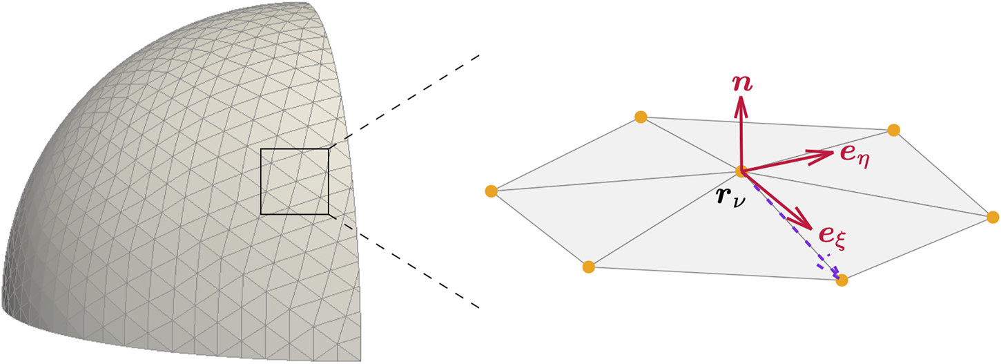
FIGURE 1. Cortex discretization. Discretization of a thin shell by nodes connected to triangles (left). For each node ${\mathit{r}}_{\mathit{\nu }}$, a local coordinate system with in-plane coordinate vectors ${\mathit{e}}_{\mathit{\xi }}$, ${\mathit{e}}_{\mathit{\eta }}$ and normal vector n is constructed. The velocity field, its derivatives and the force balance equations can be expressed in this local coordinate system (${\mathit{e}}_{\mathit{\xi }},{\mathit{e}}_{\mathit{\eta }},\mathit{n}$) at the position ${\mathit{r}}_{\mathit{\nu }}$.

The local curvature tensor at the position of the central node expressed in the local coordinate system (Eq. 30) can be obtained by a parabolic fitting procedure with respect to node position as detailed in Ref. [42].

The active surface stress of the cortex is considered to be known, as detailed above, and its distribution can be described by an analytically tractable form on the initial shape of the cortex. As detailed in Ref. [42] the active surface stress distribution is therefore prescribed on the initial shape of the cortex for each node and afterwards advected with each node.

The key quantity of interest, the velocity v, is a three-dimensional vector in the three-dimensional Cartesian space

$\mathit{v}=v^x{\mathit{e}}_x+v^y{\mathit{e}}_y+v^z{\mathit{e}}_z,(31)$

with e_i, i = x, y, z the Cartesian unit coordinate vectors. Because the velocity field is defined on the thin shell, we can evaluate the velocity at each node ν giving $v_{\nu }^i=v^i({\mathit{r}}_{\nu })$. In total, the velocity field consists of the velocity of each node

$\begin{array}{cc}\hfill v^x& ={\{v_{\nu }^x\}}_{\nu \in \{0;\dots ;N-1\}},\hfill \\ \hfill v^y& ={\{v_{\nu }^y\}}_{\nu \in \{0;\dots ;N-1\}},\hfill \\ \hfill v^z& ={\{v_{\nu }^z\}}_{\nu \in \{0;\dots ;N-1\}}.\hfill \end{array}(32)$

The velocity components in the local coordinate system Eq. 30 can easily be obtained by projection onto the corresponding local coordinate vectors according to Eq. 6

$v_{\xi }=\mathit{v}\cdot {\mathit{e}}_{\xi },v_{\eta }=\mathit{v}\cdot {\mathit{e}}_{\eta },v^n=\mathit{v}\cdot \mathit{n}.(33)$

With the derivatives of the velocity vector as introduced in Eq. 18 being evaluated in local coordinates, i.e., A_v = ∇_ξv, …, E_v = ∇_ξ∇_ηv, we can write down the velocity gradient Eq. 10 in the local coordinate system, e.g., the component

$v_{\xi \eta }=\frac{1}{2}\left[{\mathit{A}}_v\cdot {\mathit{e}}_{\eta }+{\mathit{B}}_v\cdot {\mathit{e}}_{\xi }\right].$

For the actual calculation of the derivatives of the velocity vector we refer to section 3.5. Using the derivatives of the velocity and the velocity gradient in local coordinates, we are able to write down the force balance Eqs 16, 17 for each node ν in its local coordinate system, which corresponds to Eqs 26–28. Considering the tangential force balance Eqs 26, 27 together with the normal force balance Eq. 28, we end up with three differential equations. These we refer to in the following by its left hand side, which depends on the velocity vectors v_ν, and by the right hand side, which does not depend on the velocity vectors. Therefore we have three coupled differential equations which the velocity field has to fulfill

$\begin{array}{cc}\hfill {\text{l.h.s.}}_1^{\nu }& ={\text{r.h.s.}}_1^{\nu },\hfill \\ \hfill {\text{l.h.s.}}_2^{\nu }& ={\text{r.h.s.}}_2^{\nu },\hfill \\ \hfill {\text{l.h.s.}}_n^{\nu }& ={\text{r.h.s.}}_n^{\nu },\hfill \end{array}(34)$

where the index 1,2 labels the two tangential force balance equations and the index n labels the normal force balance equation. The superscript ν emphasizes that we refer to the equation in local coordinates of node ν, which is the force balance evaluated at position r_ν of node ν.

3.2 Constraints

Since only derivatives of the velocity field occur in the force balance equations, an arbitrary constant velocity can be added without violating the force balance equations. Furthermore, these derivatives are directional and under certain circumstances, e.g., axisymmetry, a velocity in azimuthal direction can be added. Therefore, we need to specify certain constraints to the velocity field, which correspond to boundary conditions for the partial differential equations.

First, we use a vanishing total normal velocity vⁿ which corresponds to an incompressible liquid inside the cell, i.e.,

$\underset{S}{\int }\mathit{v}\cdot \mathit{n}\mathrm{d}S=\sum _{\nu =0}^{N-1}{\mathit{v}}_{\nu }\cdot \mathit{n}{A}_{\nu }=0,(35)$

where the first equality results from the discretization of the integral into a sum over all nodes ν with A_ν being the local area of node ν. The local area is calculated using Meyer’s mixed area [42, 69]. This constraint of incompressibility accompanies the pressure difference P introduced in the normal force balance Eq. 17.

Second, we use that the total velocity of the cortex vanishes, i.e.,

$\underset{S}{\int }\mathit{v}\mathrm{d}S=\sum _{\nu =0}^{N-1}{\mathit{v}}_{\nu }{A}_{\nu }=\mathit{0}.(36)$

This constraint resolves the fact that due to the lack of an external force acting on the cortex the solution of the force balance equations is invariant under solid translation. In case of cell movement, one has to consider an additional coupling to the environment leading to additional external forces, for example via a friction coefficient in case of amoeboid motion [70] and in that case this constraint is lifted.

Third, we use with analogous motivation the fact that the effective total angular momentum of the cortex vanishes, i.e.,

$\underset{S}{\int }\mathit{r}\times \mathit{v}\mathrm{d}S=\sum _{\nu =0}^{N-1}{\mathit{r}}_{\nu }\times {\mathit{v}}_{\nu }{A}_{\nu }=\mathit{0},(37)$

in order to tackle the invariance under solid rotation. Again, in presence of additional external torques this constraint has to be lifted.

3.3 Minimization Ansatz for the Force Balance

The overall goal is to solve the force balance equations for the velocity field. Accompanied by the incompressibility constraint from the cytoplasm, we also solve for the pressure. Since the solution fulfills the force balance on the complete thin shell, the force balance equations must be fulfilled at every node r_ν. Using Eq. 34, we define

${\chi }^2=\sum _{\nu }\left[{({\text{l.h.s.}}_1^{\nu }-{\text{r.h.s.}}_1^{\nu })}^2+{({\text{l.h.s.}}_2^{\nu }-{\text{r.h.s.}}_2^{\nu })}^2+{({\text{l.h.s.}}_n^{\nu }-{\text{r.h.s.}}_n^{\nu })}^2\right],(38)$

taking the two tangential and the normal force balance equation into account, with the sum $\sum _{\nu }$ over all nodes. The χ² vanishes for the exact solution of the force balance equations by construction.

In order to incorporate the constraints detailed in the previous section 3.2, we use the concept of Lagrange multipliers. The incompressibility constraint Eq. 35 imposes one condition whereas the constraints in Eqs 36, 37 each impose three conditions due to the three components of the velocity vector. For each of the conditions we introduce a separate Lagrange multiplier. The constraint times the Lagrange multiplier is added to the χ² in Eq. 38, e.g.,

$\begin{array}{cc}\hfill {\chi }^2=\sum _{\rho }\sum _{\nu }{\left({\text{l.h.s.}}_{\rho }^{\nu }-{\text{r.h.s.}}_{\rho }^{\nu }\right)}^2& +{\lambda }_1\left(\sum _{\nu =0}^{N-1}{v}_{\nu }^x{A}_{\nu }-0\right)+{\lambda }_2\left(\sum _{\nu =0}^{N-1}{v}_{\nu }^y{A}_{\nu }-0\right)\hfill \\ \hfill & +{\lambda }_3\left(\sum _{\nu =0}^{N-1}{v}_{\nu }^z{A}_{\nu }-0\right),\hfill \end{array}(39)$

for the total velocity constraint Eq. 36 as illustration and with ρ = 1, 2, n.

For the exact solution the χ² would become zero, numerically we seek the minimum of χ². Thus, in simulations we have to solve for the velocity set $v_{\nu }^x,v_{\nu }^y,v_{\nu }^z$ in Eq. 32 together with the pressure difference P, which minimizes χ². We therefore have to calculate

$\underset{\{{\mathit{v}}_{\nu }\},P}{\arg \min }{\chi }^2=\underset{\{v_{\nu }^x\},\{v_{\nu }^y\},\{v_{\nu }^z\},P}{\arg \min }{\chi }^2.(40)$

In order to perform this minimization, we calculate the derivatives of χ² with respect to the velocity components of each node $v_{\nu }^i$ and with respect to P. Due to minimization the derivatives equal zero and we can separate this equality for terms linear in $v_{\nu }^i$, P and terms independent of the velocity or pressure, where we use the parabolic expansion of the velocity field in Eq. 18. In total, this leads to a system of linear equations in matrix form with dimensions (3N + 1) × (3N + 1). There we have 3N rows due to the derivatives w.r.t. to the N velocities with 3 components each and we have 3N columns due to the N velocities with 3 components each in the solution vector. In addition, we have a row and a column due to the derivative with respect to and the dependency on the pressure, respectively. In the minimization procedure in Eq. 40, each Lagrange multiplier enters as an additional unknown, thus adding one row (containing derivatives w.r.t. the Lagrange mulitplier $\frac{\partial {\chi }^2}{\partial {\lambda }_j}$) and one column containing the coefficients of λ_j.

In order to calculate the corresponding matrix to the system of linear equations we have to evaluate the left hand side and right hand side of all three force balance equations on each node in the local coordinate system Eq. 30. This we do using the velocity derivatives in local coordinates as detailed in 3.1. For details on the dependency on the actual velocity values we refer to section 3.6. The system of equations can finally be solved numerically using LU-Decomposition.

3.4 Improving Numerical Stability by an Artificial Bending Viscosity

The velocity field in the cell cortex advects the cortex material and thus determines its reorganization and changes in shape over time. While tangential flows are parallel to the current shape, the normal velocity leads to a deformation of the cortex shape. For reasons of numerical stability, we consider here an additional damping contribution to the surface stress tensor which is similar to a bending viscosity [40]. The aim of this additional bending contribution, which is chosen to be small, is to include a condition on the second derivative of the normal velocity, which does not appear in the force balance equations. Due to its smallness and the limitations of the parabolic expansion we neglect the contribution of the bending contribution to the tangential force balance equations. The normal component of the velocity is obtained from the three-dimensional velocity by projection onto the normal vector Eq. 6. Derivatives are again obtained using a parabolic expansion similar to Eq. 18. We consider the time derivative of the curvature tensor in the Eulerian frame according to Salbreux and Jülicher [40].

${\partial }_t{C}_{\alpha }^{\beta }=-{\nabla }_{\alpha }{\nabla }^{\beta }{v}^n-v^n{C}_{\alpha \gamma }{C}^{\beta \gamma },(41)$

and the derivative of the trace

${\partial }_t{C}_{\gamma }^{\gamma }=-{\nabla }_{\gamma }{\nabla }^{\gamma }{v}^n-v^n{C}_{\gamma \delta }^{}{C}^{\gamma \delta }=-{\nabla }_{\gamma }{\nabla }^{\gamma }{v}^n-v^n{C}_{\gamma }^{\delta }{C}_{\delta }^{\gamma }.(42)$

Using the expressions above, an additional in-plane surface stress related to a bending $\bar{\eta }$ and bending bulk ${\bar{\eta }}_b$ viscosity, which account for dissipation due to curvature changes [40], is chosen as

$\begin{array}{ll}\hfill t_{\text{b}}^{\alpha \beta }& =2\bar{\eta }{g}^{\alpha \gamma }\left[{\partial }_t\left(C_{\gamma }^{\beta }-\frac{1}{2}{C}_{\delta }^{\delta }{\delta }_{\gamma }^{\beta }\right)-C_{\delta }^{\delta }{v}^n{C}_{\gamma }^{\beta }\right]+{\bar{\eta }}_b\left({\partial }_t{C}_{\gamma }^{\gamma }\right)g^{\alpha \beta }\hfill \\ \hfill & =2\bar{\eta }\left(-{\nabla }^{\alpha }{\nabla }^{\beta }{v}^n-v^n{C}_{\gamma }^{\alpha }{C}^{\beta \gamma }-C_{\gamma }^{\gamma }{v}_n{C}^{\alpha \beta }\right)+\left({\bar{\eta }}_b-\bar{\eta }\right)\left(-{\nabla }_{\gamma }{\nabla }^{\gamma }{v}^n-v^n{C}_{\gamma }^{\delta }{C}_{\delta }^{\gamma }\right)g^{\alpha \beta }.\hfill \end{array}$

In Ref. [40] a contribution due to effective bending viscosities is introduced for a thin shell with broken up-down-symmetry and the bending viscosity can be negative. Again, we note that its addition here, in our three-dimensional framework, with an additional factor involving the normal velocity is motivated by reasons of numerical stability. The normal force balance contribution is calculated by contraction with the curvature tensor

$\begin{array}{ll}\hfill t_{\text{b}}^{\alpha \beta }{C}_{\alpha \beta }& =2\bar{\eta }\left(-{\nabla }_{\alpha }{\nabla }_{\beta }{v}^n-v^n{C}_{\alpha \gamma }^{}{C}_{\beta }^{\gamma }-C_{\gamma }^{\gamma }{v}_n{C}_{\alpha \beta }\right)C^{\alpha \beta }\hfill \\ \hfill & +\left({\bar{\eta }}_b-\bar{\eta }\right)\left(-{\nabla }_{\gamma }{\nabla }^{\gamma }{v}^n-v^n{C}_{\gamma }^{\delta }{C}_{\delta }^{\gamma }\right)g^{\alpha \beta }{C}_{\alpha \beta }\hfill \\ \hfill & =2\bar{\eta }\left(-{\nabla }_{\alpha }{\nabla }_{\beta }{v}^n-v^n{C}_{\alpha \gamma }^{}{C}_{\beta }^{\gamma }-C{v}_n{C}_{\alpha \beta }\right)C^{\alpha \beta }\hfill \\ \hfill & +\left({\bar{\eta }}_b-\bar{\eta }\right)\left(-{\nabla }_{\gamma }{\nabla }^{\gamma }{v}^n-v^n{C}_{\gamma }^{\delta }{C}_{\delta }^{\gamma }\right)C,\hfill \end{array}$

with C = g^αβC_αβ. With the derivatives of the normal velocity $A_{v^n},B_{v^n},\dots ,E_{v^n}$ in analogy to Eq. 18, the trace of the second derivative can be written as

${\nabla }_{\gamma }{\nabla }^{\gamma }{v}^n=g^{\alpha \beta }{\nabla }_{\alpha }{\nabla }_{\beta }{v}^n=g^{11}{C}_{v^n}+g^{22}{D}_{v^n}.(43)$

We further use

$C_{\alpha \beta }{C}^{\alpha \beta }=C_{11}{C}^{11}+2C_{12}{C}^{12}+C_{22}{C}^{22}=\tilde{C},(44)$

and

$C_{\alpha \gamma }{C}_{\beta }^{\gamma }{C}^{\alpha \beta }=\bar{C},$

to obtain in total

$\begin{array}{ll}\hfill t_{\text{b}}^{\alpha \beta }{C}_{\alpha \beta }& =\left(-2\bar{\eta }{C}^{11}-\left({\bar{\eta }}_b-\bar{\eta }\right)C{g}^{11}\right)C_{v^n}+\left(-2\bar{\eta }{C}^{22}-\left({\bar{\eta }}_b-\bar{\eta }\right)C{g}^{22}\right)D_{v^n}-4\bar{\eta }{C}^{12}{E}_{v^n}\hfill \\ \hfill & +\left(-2\bar{\eta }\bar{C}-2\bar{\eta }C\tilde{C}-\left({\bar{\eta }}_b-\bar{\eta }\right)C\tilde{C}\right)v^n.\hfill \end{array}(45)$

This contribution can be added to the normal force balance equation and can be incorporated into the solution procedure detailed above in a straightforward manner.

3.5 Velocity Derivatives as a Function of Neighboring Velocity Vectors

Up to now, we have written the force balance Eqs 26–28 in terms of derivatives of the velocity vector in local coordinates A_v, B_v, …, E_v, which themselves are three-dimensional Cartesian vectors. What remains is to express these derivatives by means of the actual velocity vectors at all nodes, which allows us to write down the force balance as system of equations that is directly solvable for the velocity. To do so, i.e., to discretize the derivatives on the numerical grid, we use a parabolic expansion. For this, we consider the neighborhood of a node as sketched in Figure 1. Considering all N_ν neighboring nodes a(ν) of node ν, the coefficients A_v, B_v, …, E_v can be expressed by the velocity vector evaluated at the central node and at the sites of the neighboring nodes

${\mathit{A}}_v={\mathit{A}}_v\left({\mathit{v}}_{\nu },\{{\mathit{v}}_{a(\nu )}\}\right)\text{with}a(\nu )=1,\dots ,N_{\nu }.(46)$

In order to do so we write down the velocity at some distance around the (central) node ν in the local coordinates of the central node ξ, η

$\bar{\mathit{v}}\left(\xi ,\eta \right)={\mathit{v}}_{\nu }+{\mathit{A}}_v\xi +{\mathit{B}}_v\eta +\frac{1}{2}{\mathit{C}}_v{\xi }^2+\frac{1}{2}{\mathit{D}}_v{\eta }^2+{\mathit{E}}_v\xi \eta ,(47)$

which is the parabolic expansion Eq. 18 evaluated in the local coordinate system Eq. 30. The position vector can be evaluated at the position of the N_ν neighboring nodes in the local coordinates of the central node, i.e., ξ_a(ν), η_a(ν), which are obtained by projection of the difference vector between the two nodes onto the local coordinate vectors. The expanded velocity at the position of the neighbors then has to be equal to the actual velocity v_a of the neighbor node a(ν). Therefore, the squared difference of expanded and actual velocity has to be minimal

${\chi }_v^2=\sum _{a=1}^{N_{\nu }}{\left[\bar{\mathit{v}}\left({\xi }_{a(\nu )},{\eta }_{a(\nu )}\right)-{\mathit{v}}_a\right]}^2.(48)$

The minimization is performed analytically in several steps, which are outlined here and detailed in the Supplementary Appendix S1. Using the differential form of Eq. 48 we calculate the derivatives with respect to A_v, B_v, …, E_v that have to equal zero due to minimization. This results in a system of linear equations expressed in terms of a 5 × 5 matrix for each of the three vector components with the velocity derivatives forming the solution vector. We invert the matrix analytically using Mathematica. By means of the inverse matrix we are able to write down the velocity derivatives A_v, B_v, …, E_v in terms of the velocity values, as illustrated by Eq. 46.

3.6 Summary of the Algorithm

Putting everything of the above together, we here summarize our numerical algorithm. Starting from a prescribed active surface stress distribution ${\zeta }_{\alpha }^{\beta }$ on the initial shape of the cortex, we compute the velocity in the cortex in Cartesian coordinates v by the following steps.

1) evaluate the active surface stress ${\zeta }_{\alpha }^{\beta }$ on the nodes of the discretized cortex and construct a local coordinate system for each node.

2) compute derivatives of the active surface stress ${\zeta }_{\alpha }^{\beta }$ together with the metric and curvature tensor at each node using a parabolic fitting for the active surface stress or the position vector, respectively, analogous to Eq. 18.

3) use the inverse parabolic fitting detailed in Supplementary Appendix S1 to obtain the derivatives of the velocity vector up to second order A_v, B_v, …, E_v in local coordinates at each node. These are functions of the (up to now) unknown velocity values at the node and its neighbors, e.g., ${\mathit{A}}_v={\mathit{A}}_v\left({\mathit{v}}_{\nu },\{{\mathit{v}}_{a(\nu )}\}\right)$.

4) use these derivatives to express the force balance equations Eqs 26–28 in terms of the velocity components of all nodes [including bending contribution Eq. 45 if applicable].

5) construct the χ² function Eq. 40 and build the corresponding matrix by taking derivatives w.r.t. the unknowns.

6) solve the corresponding linear system for the velocity field {v_ν}, the pressure P and the Lagrange multipliers.

4 Validation and Application

In the following, we intensively validate the developed algorithm for a viscous active cell cortex in three dimensions. First, we consider in section 4.1 a static spherical cortex subjected to an active surface stress distribution in terms of spherical harmonics. We compare the resulting velocity field on the cortex to analytical solutions derived in Supplementary Appendix S2. Next, we compare our three-dimensional simulations for a dynamically deforming cortex to axisymmetric simulations in section 4.2. Finally, we exploit the capabilities of our fully 3D algorithm to study fold formation in section 4.3 as well as furrow formation under non-axisymmetric external perturbations in section 4.4.

4.1 Velocity Profile by Spherical Harmonics on a Static Spherical Cortex

As a first test setup, we compare three-dimensional numerical results on a static spherical cortex to corresponding analytical solutions. We consider an isotropic active surface stress distribution across the cortex

${\zeta }^{\alpha \beta }(\theta ,\varphi )=\zeta (\theta ,\varphi )g^{\alpha \beta }(49)$

which is analytically expanded in terms of spherical harmonics Y_lm (θ, ϕ)

${\zeta }^{\alpha \beta }(\theta ,\varphi )=\zeta (\theta ,\varphi )g^{\alpha \beta }=\sum _{l=0}^{\infty }\sum _{m=-l}^l{\zeta }_{lm}{Y}_{lm}(\theta ,\varphi )g^{\alpha \beta },(50)$

where ζ_lm are the expansion coefficients of the active surface stress distribution. Here, greek indices denote the two angles of spherical coordinates θ and φ. For the given active surface stress profile in Eq. 50, we derive an analytical solution for the velocity field v in Supplementary Appendix S2. We expand the tangential velocity in terms of vector spherical harmonics ${\mathit{v}}^t=\sum _{l,m}{v}_{lm}^1{\partial }_{\alpha }{Y}_{lm}{\mathit{e}}^{\alpha }$ with coefficients $v_{lm}^1$ (we note here that the component in direction $\mathit{n}\times \left({\partial }_{\alpha }{Y}_{lm}\right){\mathit{e}}^{\alpha }$ vanishes as discussed in the Supplementary Appendix S2) and the normal velocity in terms of spherical harmonics $v^n=\sum _{l,m}{v}_{lm}^n{Y}_{lm}$ with coefficients $v_{lm}^n$. The force balance equations Eq. 16, Eq. 17 then lead to analytical relations for the velocity expansion coefficients $v_{lm}^1$ and $v_{lm}^n$ depending on ζ_lm. These relations are given in Supplementary Equations S2.23, S2.25 and determine the velocity field. In the following, we consider the quantities in units of the inital cortex radius R₀ and the planar shear viscosity thus fixing R =R₀=1 and η_s = 1. In the following, we consider the results for l >1. On the one hand, considering the full system of equations (case i)), the difference of the conditions Supplementary Equations (S2.23) and (S2.25) implies a vanishing in-plane velocity, i.e., the expansion coefficients of the in-plane velocity vanish

$v_{lm}^{\left.1,\mathrm{i}\right)}=0.(51)$

In turn, the normal velocity has to fulfill Supplementary Equation S2.27 which leads to

$v_{lm}^{\left.n,\mathrm{i}\right)}=-\frac{R}{2{\eta }_b}{\zeta }_{lm}.(52)$

In summary, the solution for the velocity field for given active surface stress ζ_lm is

${\mathit{v}}^{\left.\mathrm{i}\right)}=-\frac{R}{2{\eta }_b}{\zeta }_{lm}{Y}_{lm}\mathit{n},(53)$

with vanishing tangential component.

On the other hand, this system can be utilized to test the in-plane velocity separately (case ii). To do so, we consider vanishing bulk viscosity η_b = 0 and fix the normal velocity vⁿ to zero. The latter implies

$v_{lm}^{\left.n,\mathrm{i}\mathrm{i}\right)}=0,(54)$

instead of solving the normal force balance. In this case, the tangential force balance equations lead to the condition (Supplementary Equation S2.28) for the tangential velocity coefficients which become

$v_{lm}^{\left.1,\mathrm{i}\mathrm{i}\right)}=\frac{1}{\left[l(l+1)-2\right]}{\zeta }_{lm}.(55)$

Thus, for solving the tangential force balance equation only in case of a vanishing normal velocity, we obtain an analytical solution for the velocity

${\mathit{v}}^{\left.\mathrm{i}\mathrm{i}\right)}=v_{lm}^{\left.1,\mathrm{i}\mathrm{i}\right)}\left({\partial }_{\alpha }{Y}_{lm}\right){\mathit{e}}^{\alpha }=\frac{1}{\left[l(l+1)-2\right]}{\zeta }_{lm}\left({\partial }_{\alpha }{Y}_{lm}\right){\mathit{e}}^{\alpha },(56)$

which is due to a given active surface stress with coefficient ζ_lm.

In both cases, the analytical solution in Eq. 53 for 1) the full system and in Eq. 56 for 2) the pure tangential system allows a direct comparison between the analytical and numerical solution. Using the three-dimensional algorithm developed above, we consider a discrete cortex with 2562 nodes and 5120 triangles without bending viscosity. After applying an active surface stress distribution in terms of spherical harmonics according to Eq. 50, we solve numerically for the three-dimensional velocity field. In case 2) the normal force balance equation entering the minimization ansatz can be replaced by the condition of vanishing normal velocity on each node. In the following, the comparison to the analytical solution is performed by considering two types of error measures. On the one hand, we consider the absolute value of the difference between numerical v and analytical solution v^an per node and average over all nodes

$⟨ϵ⟩=\frac{1}{N}\sum _{\nu }|\mathit{v}-{\mathit{v}}^{\text{an}}|.(57)$

On the other hand, we calculate the sum of the squared difference of the velocities relative to the maximum velocity, average, and take the square root to obtain the relative error

${ϵ}_{\text{rel}}=\sqrt{\frac{\frac{1}{N}\sum _{\nu }\left[{\left(v_x-v_x^{\text{an}}\right)}^2+{\left(v_y-v_y^{\text{an}}\right)}^2+{\left(v_z-v_z^{\text{an}}\right)}^2\right]}{||{\mathit{v}}^{\text{an,\hspace{0.17em}max}}||}}.(58)$

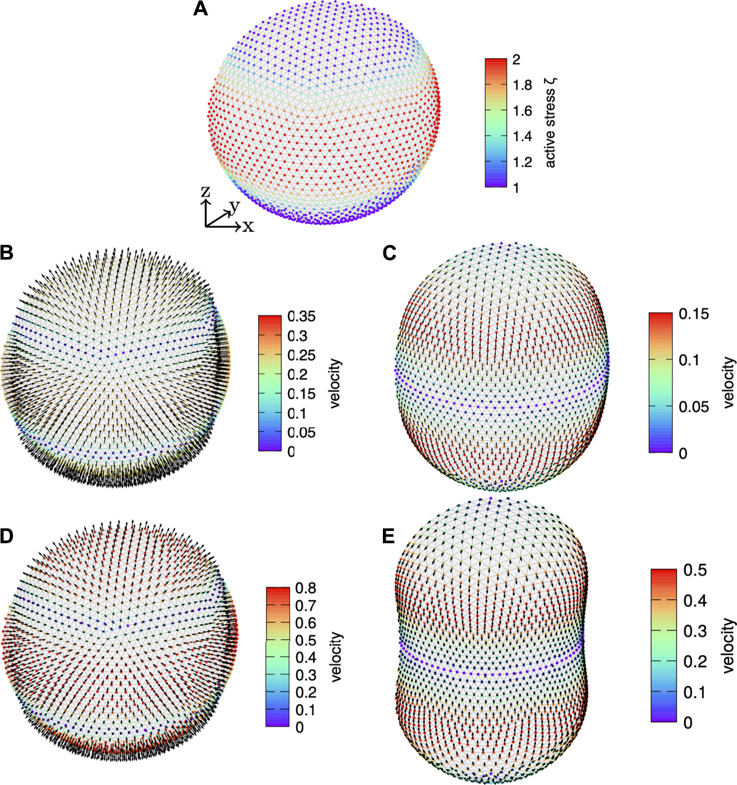
We first consider an axisymmetric active surface stress distribution in terms of ζ₂₀Y₂₀ with ζ₂₀ = 1 as shown in Figure 2A) on the discrete cortex. We further use η_b = 1 and an active surface stress offset of ζ₀₀ = 0. A variation of the active surface stress offset leads to a finite pressure difference, but the velocity field is not altered. Figures 2B–E shows the full, three-dimensional velocity profile obtained numerically with the velocity magnitude per node color coded and the velocity direction indicated by arrows and the velocity depending on the polar angle θ in comparison to the analytical solution for both systems. In system 1), the normal velocity is finite and points outward the cell around the equator and inward at both poles. In system 2), the tangential velocity is finite and directed from the equator towards the poles. Each three-dimensional simulation shows very good agreement with the analytical solution, as shown by the comparison over the polar angle. As a next step, we quantify the error ⟨ϵ⟩ as well as ϵ_rel given in Eqs 57, 58, respectively, and vary the resolution of the discrete spherical cortex. As shown in Figures 2F,G, we obtain a systematic decrease of both errors with increasing resolution for both systems. The error shows a scaling inversely proportional to the number of nodes.

FIGURE 2

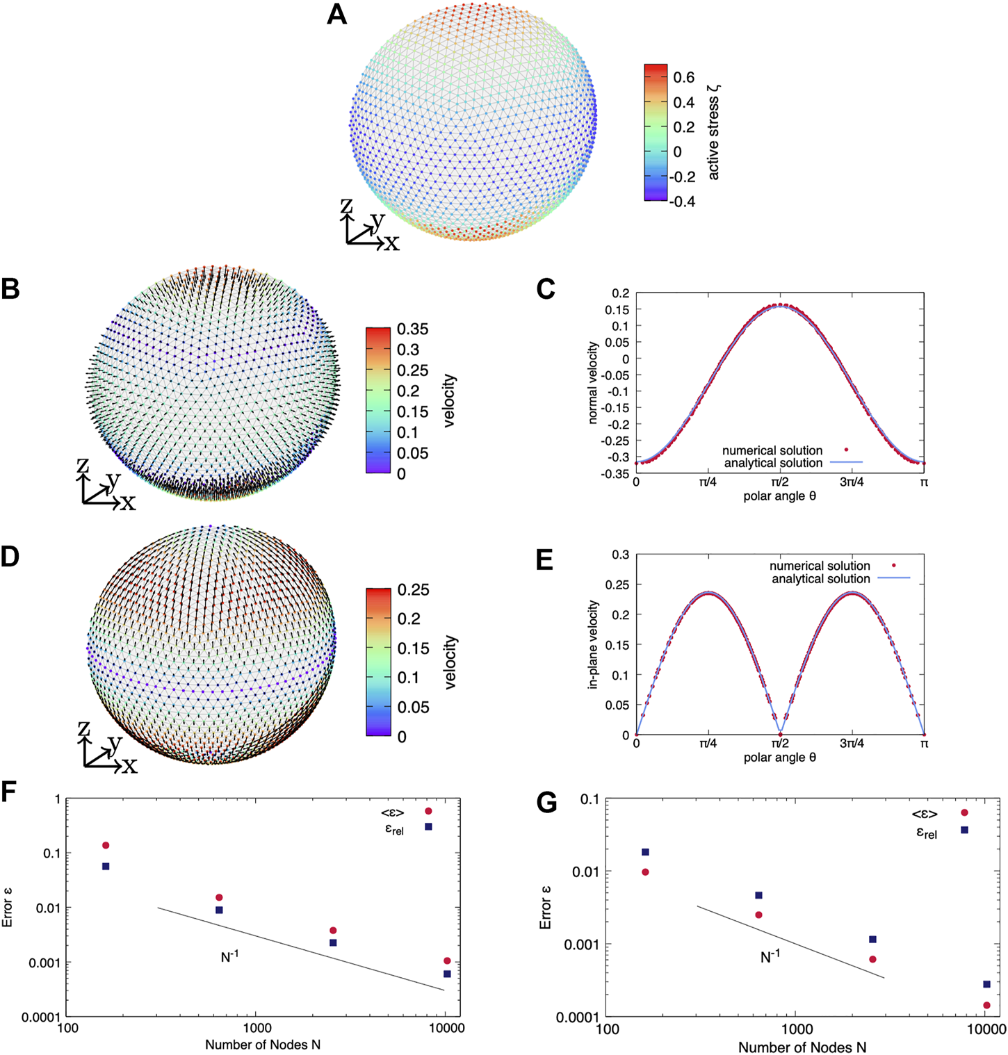
FIGURE 2. Axisymmetric active surface stress on a static spherical cortex. (A) An axisymmetric active surface stress distribution in terms of $Y_{20}$ is considered on a spherical cortex. In (B,C) the full system (case i) is solved whereas (D,E) show the purely tangential system (case ii). (B) The three-dimensional velocity field is shown as obtained by the numerical solution of the full system. (C) While the tangential velocity is zero, the normal velocity depending on the polar angle $\theta$ agrees very well with the analytical prediction. (D) The three-dimensional velocity field is shown as obtained by the numerical solution for solving the tangential force balance only. (E) While the normal velocity is zero, the absolute value of the tangential velocity depending on the polar angle $\theta$ agrees very well with the analytical prediction. For both the full system i) in (F) and the purely tangential system ii) in (G), the error of the velocity converges with increasing resolution.

We then proceed in Figure 3 with a non-axisymmetric distribution of active surface stress in terms of ζ₂₁Y₂₁ with ζ₂₁ = 1 and ${\zeta }_{00}=\sqrt{4\pi }$ shown in Figure 3A. Again, we show the full system i) in Figures 3B,C and the purely tangential system ii) in Figures 3D,E. As a consequence of the non-axisymmetric active surface stress distribution, the cortical velocity profile is no longer axisymmetric. Figure 3B shows the three-dimensional velocity field for the full system i) and Figure 3D shows the three-dimensional velocity field for the purely tangential system ii) with normal velocity restricted to zero. Figure 3B shows four patches of large normal velocity. Opposite patches show either an outward or an inward pointing normal velocity. In-between, the normal velocity becomes zero. At the sites where in Figure 3B the normal velocity is maximal, the tangential velocity in Figure 3C vanishes. Similar to Figure 2 the tangential velocity points from sites with outward pointing normal velocity towards sites with inward pointing normal velocity in Figure 3B. In Figures 3C,E we compare the numerically obtained velocity to the analytical solution by showing the velocity value depending on the polar angle θ for an azimuthal angle ϕ = 0. Again, we observe very good agreement between numerical and analytical solution and a systematic convergence with increasing number of nodes as shown in Figures 3F,G for both systems i) and ii), respectively.

FIGURE 3

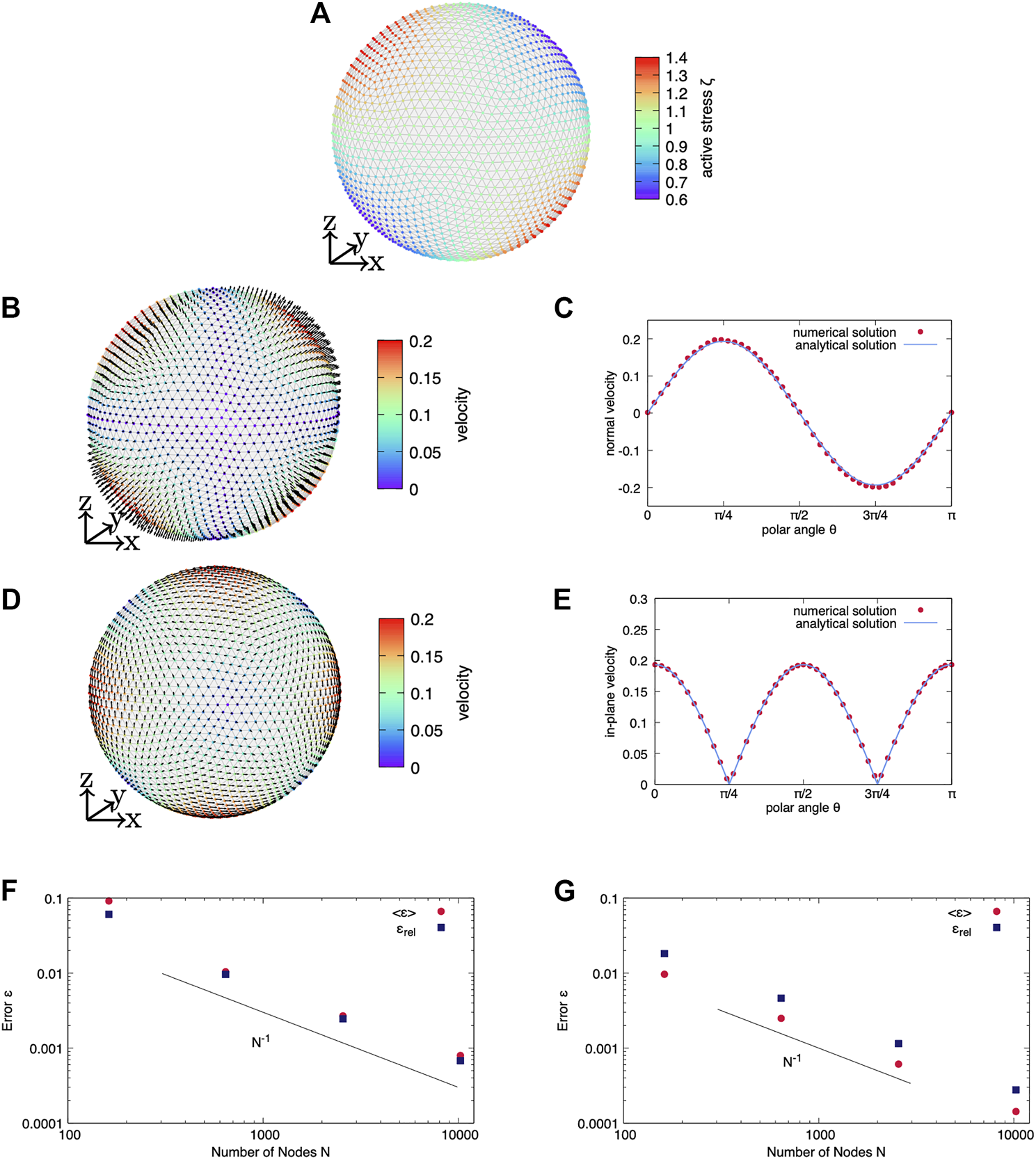
FIGURE 3. Non-axisymmetric active stress. (A) A non-axisymmetric active surface stress distribution in terms of Y₂₁ is considered. In (B,C) the full system (case i) is solved whereas (D,E) show the purely tangential system (case ii). (B) The numerically obtained three-dimensional velocity feld is shown for i) the full system. (C) While the tangential velocity is zero, the normal velocity depending on the polar angle $\theta$ shown for $\varphi =0$ agrees very well with the analytical prediction. (D) The numerically obtained three-dimensional velocity field is shown for ii) solving the tangential force balance only. (E) While the normal velocity is zero, the absolute value of the tangential velocity depending on the polar angle $\theta$ shown for $\varphi =0$ agrees very well with the analytical prediction. The error (F) of the normal velocity for the full system i) as well as (G) the error of the tangential velocity for the reduced system of tangential force balance ii) converges with increasing resolution.

4.2 Dynamics of an Axisymmetric Viscous Active Cortex

Having tested the algorithm for the static scenario in the previous section, we now apply our method to a dynamically evolving viscous active cortex immersed in a passive outer fluid. We consider an active surface stress distribution similar to what is known for cytokinesis, i.e., the separation of the two daughter cells by an evolving cleavage furrow during cell division [30, 32, 33, 46]. Initially, on the undeformed spherical cortex, we consider an active surface stress that is isotropic with constant offset ζ₀ at the poles and increases towards the equator to form a contractile ring

${\zeta }_1^1(\theta ,\varphi )={\zeta }_2^2(\theta ,\varphi )=\zeta (\theta ,\varphi )={\zeta }_0+\widehat{\zeta }\exp \left(-\sigma {\left(\theta -\frac{\pi }{2}\right)}^p\right),(59)$

where $\widehat{\zeta }$ is the amplitude of active surface stress increase around the equator, p the exponent, and σ the width of the active surface stress distribution. Again we use R = 1 and for the active surface stress we fix ζ₀ = 1, σ = 10, retaining the planar shear and bulk viscosity as η_s = η_b = 1. The exponent p is varied. We use an initially spherical mesh with 2562 nodes and 5120 triangles.

For the given active surface stress distribution in Eq. 59 and for given cortex shape, we solve numerically for the three-dimensional velocity field v on the discrete cortex. We split up the total velocity field v into the tangential velocity ${\mathit{v}}_t=\left(\mathit{1}-\mathit{n}\otimes \mathit{n}\right)\cdot \mathit{v}$ and the normal velocity ${\mathit{v}}_n=\left(\mathit{n}\otimes \mathit{n}\right)\cdot \mathit{v}$. Since only the normal velocity leads to flows in the cortex that change the overall cortex shape, we integrate the cortex evolution similar to Refs. [45, 71] by advecting each node ν with its normal velocity ${\mathit{v}}_n^{\nu }$. With this, a numerically demanding re-meshing, which would be necessary in case of tangential advection of the mesh nodes, is avoided. Advection is carried out using the Euler algorithm

${\mathit{r}}_{\nu }(t+\mathrm{\Delta }t)={\mathit{r}}_{\nu }(t)+{\mathit{v}}_n^{\nu }(t)\mathrm{\Delta }t,(60)$

with a time step Δt, which is typically chosen to be Δt = 5 × 10^–4 t_a with the time scale $t_{\text{a}}=\frac{{\eta }_s}{{\zeta }_0}$. After a number of time steps, we observe that the normal velocity on the whole cortex vanishes, i.e., the cortex has reached a final, steady state.

We first consider a broad distribution of active surface stress with exponent p = 8 in Eq. 59 with $\widehat{\zeta }=1$ as shown in Figure 4A. We apply a bending viscosity of $\bar{\eta }=0.0005{\eta }_s$ and ${\bar{\eta }}_b=0.0025{\eta }_s$. Figure 4B shows the velocity field on the initially spherical cortex. Because of the dominating contractile active surface stress around the equator, the normal velocity points towards the cell interior around the equator. As a consequence of the incompressibility of the enclosed fluid, the normal velocity points outward at the poles. Therefore, the velocity leads to an expansion of the cortex along the z-axis and a simultaneous contraction around the equator. Integration of the cortex evolution leads to the shape shown in Figure 4C, where we also show the final velocity field on the deformed cortex. Here, no normal velocity remains, but a finite tangential velocity points towards the equator.

FIGURE 4

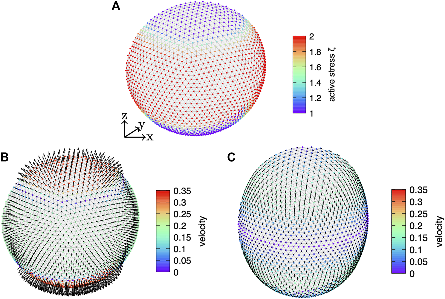
FIGURE 4. Dynamically deforming viscous active cortex. (A) The active surface stress distributed according to Eq. 59 with exponent p = 8, offset ${\zeta }_0=1$, and amplitude $\widehat{\zeta }=1$ is shown color coded on the initially spherical, discrete cortex. Towards the equator the isotropic active surface stress increases. (B) Resulting velocity profile on the initial cortex and (C) velocity after the cortex has reached its final shape where the normal velocity vanishes.

For this setup, we compare the three-dimensional dynamics to the one obtained by axisymmetric simulations of viscous active surfaces [72] in Figure 5. Details of the axisymmetric simulations are given in Supplementary Appendix S4. For comparison between the simulation methods, we track the distance between the poles, which is divided by a factor of two, as well as the radius of the furrow at the equator. Both quantities are displayed as functions of time in Figure 5A. While the pole to pole radius increases over time, the cortex contracts at the equator and thus the furrow radius decreases. Both quantities reach a constant plateau at longer time, which corresponds to the convergence of the simulation and results from the interplay of the contractile active stress at the pole and cortical ring contraction mediated by the incompressibility of the enclosed fluid [33]. We obtain excellent agreement between three-dimensional and axisymmetric simulation.

FIGURE 5

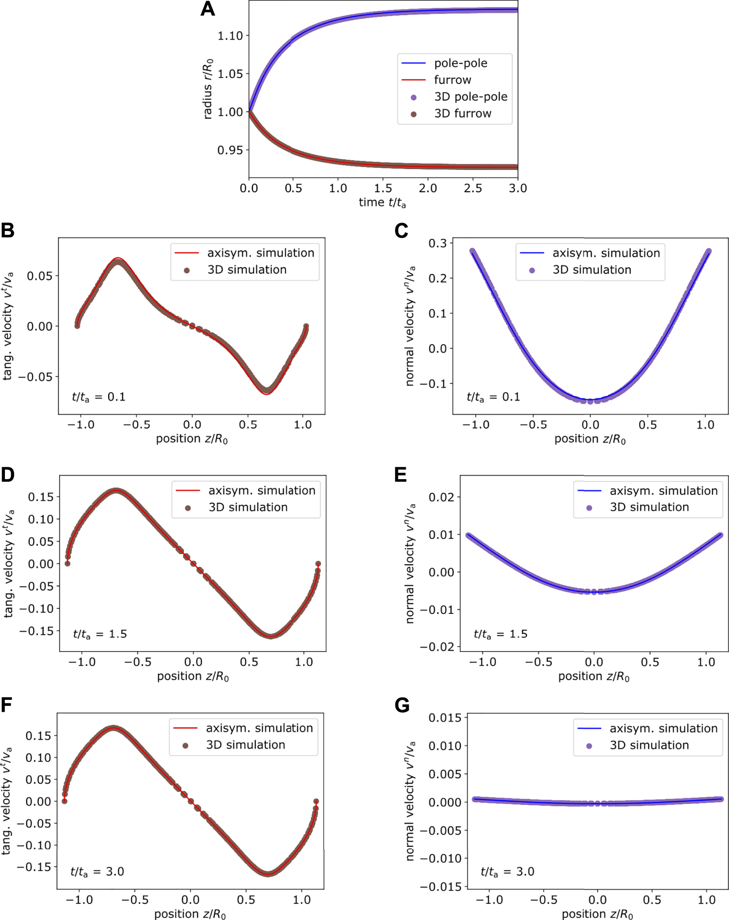
FIGURE 5. Comparison of cortex dynamics. (A) Comparison of the pole to pole and furrow radius between axisymmetric (lines) and three-dimensional (dot) simulations for the setup shown in Figure 4 with p = 8, ${\zeta }_0=1$, $\widehat{\zeta }=1$ (B–G) The tangential (left) and normal (right) velocity profile obtained from axisymmetric simulation and three-dimensional simulation is compared at different time points. Both simulation methods are in very good agreement.

To go one step further, we also compare the velocity field on the discrete cortex at different times. On the left hand side of Figure 5 we show the absolute value of the tangential velocity v_t depending on the axial position z. On the right hand side we show the normal velocity v_n. Velocities are shown at different times and are normalized by $v_{\text{a}}=\frac{R_0}{t_{\text{a}}}$. While the tangential velocity increases over time, i.e., with increasing deformation of the cortex, the normal velocity decreases until the cortex reaches its final shape (the latter is shown in Figure 4C). Overall, our developed three-dimensional algorithm leads to a velocity field on the evolving cortex, which is in very good agreement with the axisymmetric simulation.

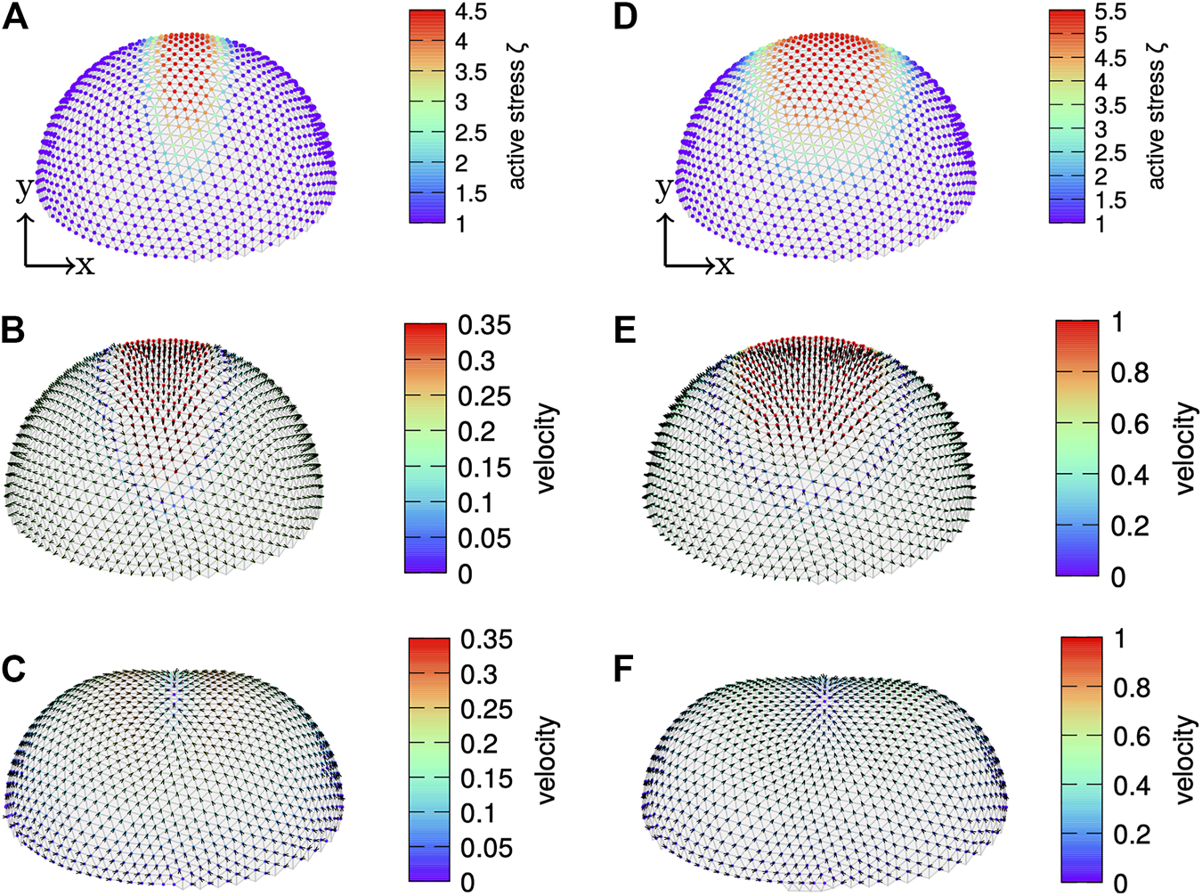
Next, we consider an active surface stress distribution around the equator, which is narrower with exponent p = 4 in Eq. 59 and systematically vary the amplitude $\widehat{\zeta }$. Figure 6 shows the active surface stress distribution for $\widehat{\zeta }=1$ as illustration in Figure 6A together with the corresponding shape and velocity profile in the Figure 6B initial and Figure 6C final state. Figures 6D,E show the initial and final state for $\widehat{\zeta }=3$. We use $\bar{\eta }=0.0005{\eta }_s$ and ${\bar{\eta }}_b=0.0025{\eta }_s$ in Figures 6A–C and $\bar{\eta }=0.0001{\eta }_s,{\bar{\eta }}_b=0.0035{\eta }_s$ in Figures 6D,E. With increasing amplitude of the active surface stress the cortex extends farther at the poles and constricts around the equator more strongly. The final tangential velocity increases systematically, which is due to the gradient in the active surface stress distribution increasing with increasing magnitude and constant offset. We again compare the dynamics based on the pole to pole and the furrow radius as well as the velocity field at different times to axisymmetric simulations. In Figure 7, we show the comparison for the amplitude $\widehat{\zeta }=1$ and in Figure 8 for $\widehat{\zeta }=3$. In all cases the results of the three-dimensional algorithm agree very well with the axisymmetric simulations.

FIGURE 6

FIGURE 6. Varying active surface stress amplitude. (A) The active surface stress distribution according to Eq. 59 with exponent p = 4, offset stress ${\zeta }_0=1$, and amplitude $\widehat{\zeta }=1$ is shown color coded on the initially spherical, discrete cortex. (B,C) Resulting velocity profile on the (B) initial cortex and on the (C) finally deformed cortex with arrows illustrating the direction and color coded magnitude. (D,E) Velocity profile for an active surface stress magnitude of $\widehat{\zeta }=3$. In the finally deformed state the normal velocity vanishes.

FIGURE 7

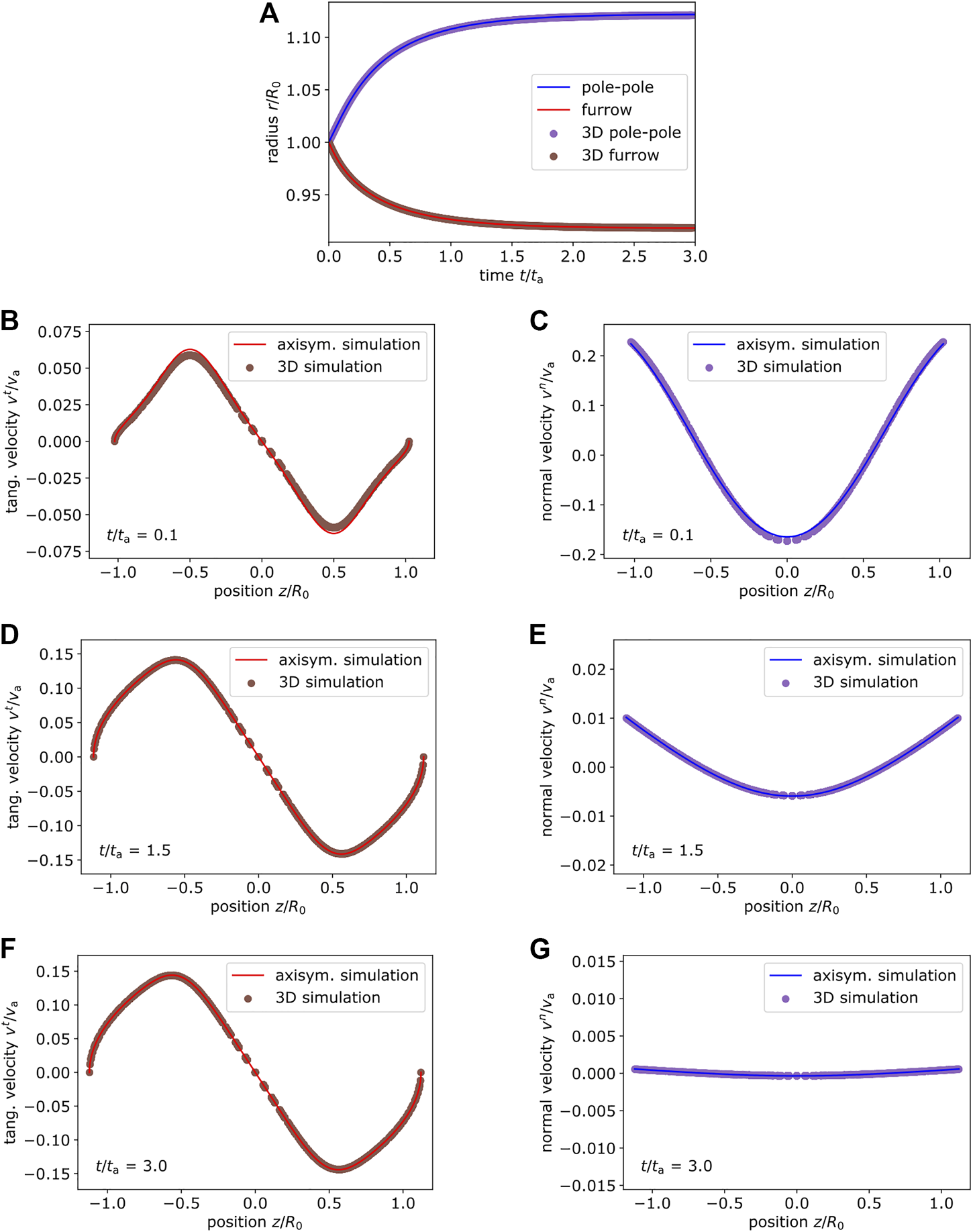
FIGURE 7. Comparison of cortex dynamics for $\widehat{\zeta }=1$. (A) Comparison of the pole to pole radius and furrow radius at the equator between axisymmetric (lines) and three-dimensional simulation (dots) for the system shown in Figure 6 (A–C) with p = 4, ${\zeta }_0=1,$ $\widehat{\zeta }=1$. (B–G) The velocity profile obtained from axisymmetric simulation and three-dimensional simulation is compared at different time points. Tangential (and normal right) velocity depending on the position $\frac{z}{R_0}$ are shown at time (B,C) $\frac{t}{t_a}=0.1$, (D,E) $\frac{t}{t_a}=1.5$, (F,G) $\frac{t}{t_a}=3$. Both simulation methods are in very good agreement.

FIGURE 8

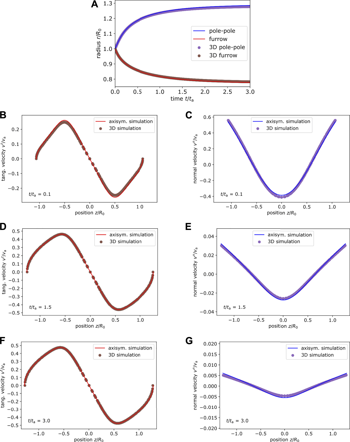
FIGURE 8. Comparison of cortex dynamics for $\widehat{\zeta }=3$. (A) Comparison of the pole to pole radius and furrow radius at the equator between axisymmetric (lines) and three-dimensional simulation (dots) for the system shown in Figure 6 (D,E) with p = 4, ${\zeta }_0=1,$ $\widehat{\zeta }=3$. (B–G) The velocity profile obtained from axisymmetric simulation and three dimensional simulation is compared at different time points. Tangential (left) and normal (right) velocity depending on the position z/R are shown at time (B,C) $\frac{t}{t_a}=0.1$, (D,E) $\frac{t}{t_a}=1.5$, (F,G) $\frac{t}{t_a}=3$. Both simulation methods are in very good agreement.

Overall, the comparison to axisymmetric simulations clearly shows the accuracy of the developed algorithm for a viscous active cortex in three dimensions also in case of dynamic cortex evolution.

4.3 Embryonic Fold Formation

As a first sample application we consider a non-axisymmetric stress pattern, which leads to the formation of a local indentation reminiscent of fold formation during embryogenesis [50]. We apply a line of increased active stress connecting both poles, which broadens towards the equator. Therefore, we modulate the active stress pattern in Eq. 59 with two additional Gaussian functions in ϕ-direction, i.e., we multiply by $\exp \left(-{\sigma }_{\varphi }{(\varphi -\pi /2)}^4\right)$ or $\exp \left(-{\sigma }_{\varphi }{(\varphi -3\pi /2)}^4\right)$, respectively. The resulting active surface stress distribution is shown in Figure 9A for $\widehat{\zeta }=3.5$ and σ_ϕ = 200 and in Figure 9D for $\widehat{\zeta }=4.5$ and σ_ϕ = 12, where in both cases ζ₀ = 1, p = 4, and σ = 1.5. We note that the cortex fulfills up-down symmetry such that we only show one half for clarity. The velocity profiles shown in Figures 9B,C,E,F, respectively, show a large initial inward velocity across the patch of enhanced active stress, where in the end Figures 9C,F a local fold forms. During fold formation an in-plane flow from the poles towards the fold develops. At the poles the cortex expands.

FIGURE 9

FIGURE 9. Fold formation. A cortex undergoing fold formation with a patch of increased active surface stress using (A–C) (left) $\widehat{\zeta }=3.5$, ${\sigma }_{\varphi }=200$ and (D–F) (right) $\widehat{\zeta }=4.5$, ${\sigma }_{\varphi }=12$. In (A,D) the active surface stress is color coded whereas in (B,C,E,F) the velocity magnitude is color coded and its direction is indicted by arrows. The upper half of the cortex is shown. The initial spherical cortex bends inwards at the patch of increased active surface stress while it extends at the poles.

4.4 Robust Cleavage Furrow Formation Under Non-axisymmetric Perturbations

In order to provide a further example application of an evolving cortex in a non-axisymmetric situation, we consider in the following a cell cortex with an initial shape that is not aligned with respect to the Cartesian coordinate axes. We use the same values for the viscosity as above, i.e., η_s = 1 and η_b = 1, an exponent p = 4 for the active surface stress distribution with constant offset ζ₀ = 1 and amplitude $\widehat{\zeta }=3.5$. For the bending viscosity we choose $\bar{\eta }=1\times 10^{-4}$ and ${\bar{\eta }}_b=5\times 10^{-3}$. Initially, we deform the cortex according to a shear strain of γ_x = 0.35 along the x-axis.

For the first setup, the active surface stress distribution is fully non-axisymmetric as shown in Figure 10A. We show in Figures 10B–E the dynamic evolution of the cortex with the velocity magnitude per node color coded and the velocity direction indicated by arrows. Initially, a large normal velocity is observed in Figure 10B with a stripe-like pattern. Roughly along the long axis of the sheared cortex the velocity points inwards the cell cortex. In direction perpendicular to the shear, the velocity points outwards of the cell cortex. This illustrates the tendency of the cell cortex to realign with respect to the symmetry of the active surface stress distribution on the undeformed cortex, which is similar to the one shown in Figure 6A. The reorientation is visible throughout the time evolution as well. Finally, the cell cortex is nearly aligned with the initial gradient of the active surface stress distribution. This points to the symmetry of the active surface stress distribution being the driving mechanism behind this reorientation. From Figures 10D,E it can be seen that the cortex subsequently contracts around the equator at the end of the reorientation. In total, this indicates that the underlying symmetry of the active surface stress distribution triggers a reorientation of the total cortex, which in the end leads to a robust furrow formation despite the initial shear disturbance. We hypothesize that in nature this autonomous reorientation may explain the robustness of cell division in noisy environments where external non-axisymmetric perturbations due to, e.g., forces by neighboring cells may be prevalent.

FIGURE 10

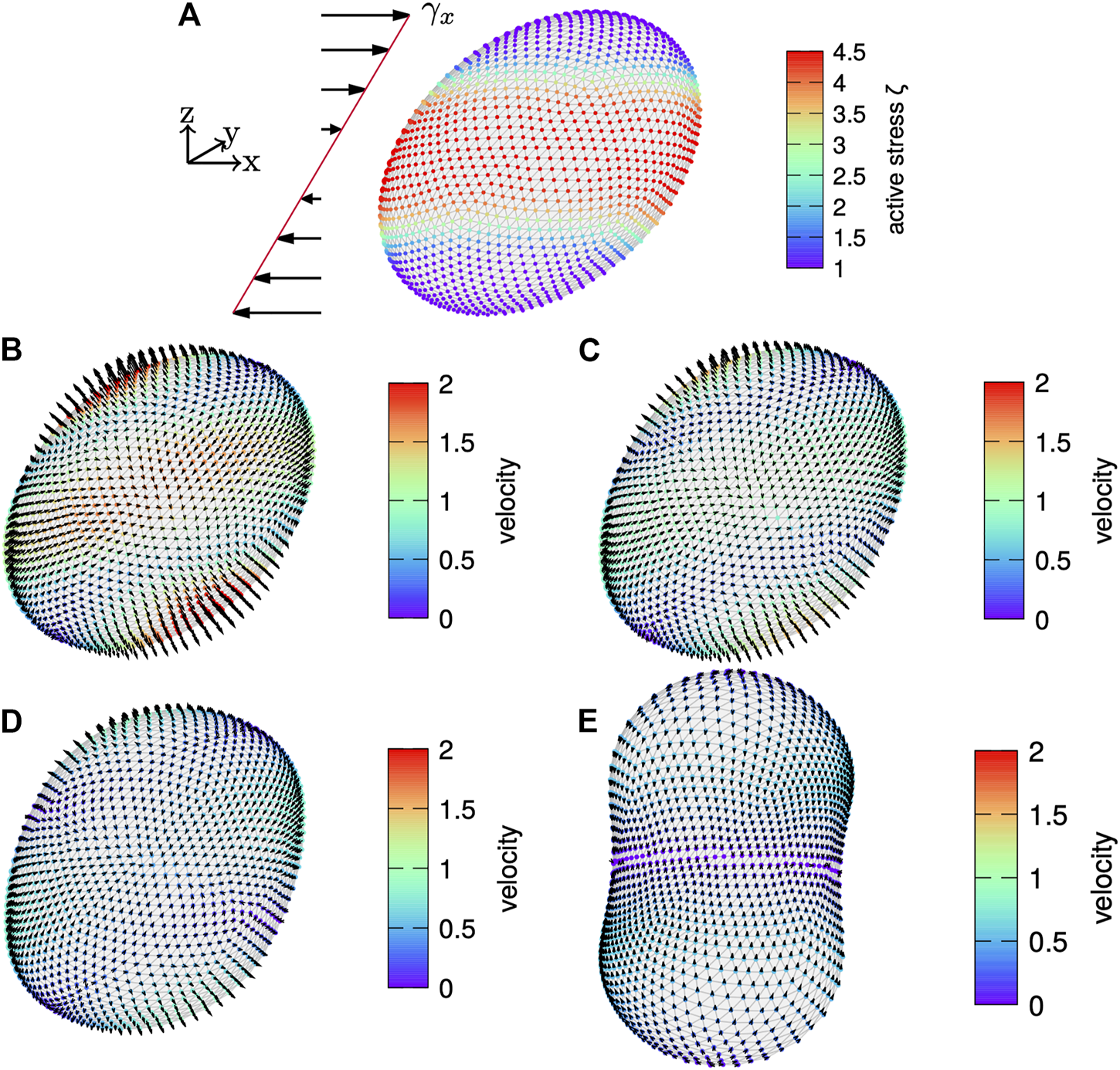
FIGURE 10. Sheared cortex. (A) A cortex subject to an initial shear of ${\gamma }_x=0.35$ is shown with the active surface stress distribution according to Eq. 59 with $\widehat{\zeta }=3.5$ color coded. The velocity field is shown on the evolving cortex over time with arrows indicating the direction and magnitude given by color code for time (B) $\frac{t}{t_a}=3.5\times 10^{-3}$, (C) $\frac{t}{t_a}=3.5\times 10^{-2}$, (D) $\frac{t}{t_a}=8.7\times 10^{-2}$ and (E) $\frac{t}{t_a}=3.5$. While the cortex contracts around the equator and extends at the poles, it relaxes back to a shape nearly oriented as the active surface stress distribution on the undeformed cortex.

In the second setup, we consider the dynamic evolution of the cortex subject to the same initial shear, but with an active surface stress distribution that is rotated such that the gradient of the active surface stress distribution nearly aligns with the shear. The initial shape is shown in Figure 11A while the evolution of the cortex is shown in Figures 11B–E at the same time points as above. Initially, the flow field shows four patches of large velocity in Figure 11B. The evolving flow field first leads to a broadening of the cortex and a slight reorientation, presumably with respect to the symmetry of the active surface stress distribution. Subsequently, the cortex contracts around the equator with the eventual shape shown in Figure 11E. The tangential velocity is directed from the poles to the equator.

FIGURE 11

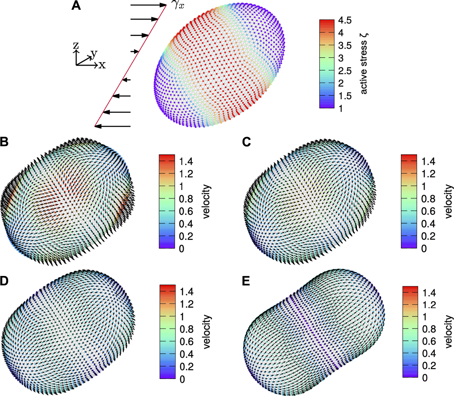
FIGURE 11. Tilted sheared cortex. (A) A cortex subject to an initial shear of ${\gamma }_x=0.35$ is shown with the active surface stress distribution according to Eq. 59 with $\widehat{\zeta }=3.5$ but rotated with an angle of 45° towards the direction of the shear color coded. The velocity field is shown on the evolving cortex over time with arrows indicating the direction and magnitude given by color code for time (B) $\frac{t}{t_a}=3.5\times 10^{-3}$, (C) $\frac{t}{t_a}=3.5\times 10^{-2}$, (D) $\frac{t}{t_a}=8.7\times 10^{-2}$ and (E) $\frac{t}{t_a}=3.5$. While the cortex contracts around the equator and extends at the poles, it retains its overall orientation.

We note that for very long times—after reaching a steady state regarding the reorientation and furrow formation—a slight asymmetry in the volume of the two daughter cells leads to an unstable shape of the dividing cell, which is due to the difference in the Laplace pressure following a difference in curvature between both regions [31, 46].

Finally, we consider about twice the shear rate, i.e., γ_x = 0.75, in Figure 12 where the results are similar to before.

FIGURE 12

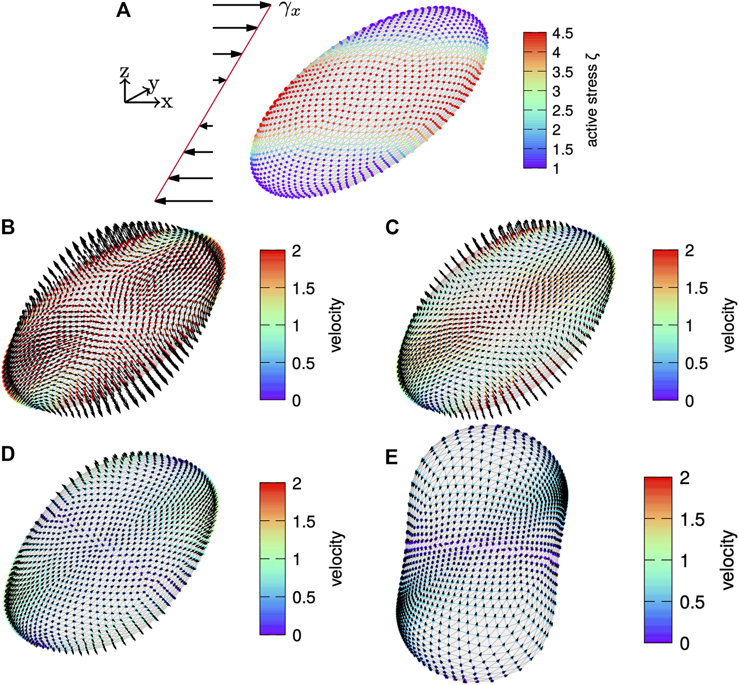
FIGURE 12. More strongly sheared cortex. (A) A cortex subject to an initial shear of ${\gamma }_x=0.75$ is shown with the active surface stress distribution according to Eq. (59) with $\widehat{\zeta }=3.5$ color coded. The velocity field is shown on the evolving cortex over time with arrows indicating the direction and magnitude given by color-code for time (B) $\frac{t}{t_a}=3.5\times 10^{-3}$, (C) $\frac{t}{t_a}=3.5\times 10^{-2}$, (D) $\frac{t}{t_a}=8.7\times 10^{-2}$ and (E) $\frac{t}{t_a}=3.5$. While the cortex contracts around the equator and extends at the poles, it relaxes back to a shape nearly oriented as the active surface stress distribution on the undeformed cortex also for this larger shear rate.

These two examples illustrate the applicability of our algorithm to non-axisymmetric situations with a three-dimensional deformation of the cortex.

5 Conclusion

In this work, we presented a simulation algorithm for the time-dependent and fully three-dimensional deformation of a viscous cell cortex including active stresses. The cell cortex is represented as a thin shell in the framework of active gel theory and discretized using a set of nodes connected by flat triangles. Using an inverted parabolic fitting procedure, we were able to express the governing force balance equations on each node in terms of the unknown velocity components. The resulting linear system is solved on the whole cortex using a global minimization ansatz. Extensive comparison to analytical solutions on a rigid sphere as well as to axisymmetric simulations of a dynamically deforming shape showed very good agreement. As first examples of non-axisymmetric situations, we considered fold formation as well as a cortex subject to a shear deformation showing a reorientation mechanism of the cortex, which can further contribute to robustness of furrow formation or cell division.

The inherent three-dimensional character of the present algorithm allows the computational investigation of more complicated scenarios of cell or tissue mechanics in the future. Especially, the robustness of cell division/furrow formation with respect to externally induced deformations, external constraints as e.g. present during embryogenesis, or even positioning of the contractile ring can be investigated in more detail. Shape changes of tissue layers triggered by active stress distributions as they occur during embryonic or cancer development can also be addressed.

The generality of the presented algorithm, which directly solves the force balance equations, allows for a straightforward inclusion of different constitutive laws for cortex behavior and active stress. By way of example, the active surface stress distribution on the discrete cortex could be derived from a concentration field and/or take into account cytoskeleton polymerization and depolymerization. Coupling to an external environment can be achieved by adding corresponding external forces to the force balance equations. Therefore, it would be possible to compute cortex dynamics inside a flowing liquid in combination with a fluid solver. Our developed numerical tool can thus be the basis for future investigations of various three-dimensional scenarios of cell and tissue morphogenesis.

Data Availability Statement

The original contributions presented in the study are included in the article/Supplementary Material. An implementation of the developed three-dimensional algorithm is available on request to the corresponding author(s). The source code for the axisymmetric simulations that has been used for validation can be found online: https://github.com/DianaKhoromskaia/AxisymCortex.

Author Contributions

CB designed the research, performed, analyzed, and interpreted the results, and wrote the article. DK performed the research and wrote the article. GS designed the research and wrote the article. SG designed the research, interpreted the results, and wrote the article.

Funding

DK and GS were supported by the Francis Crick Institute which receives its core funding from Cancer Research UK (FC001317), the UK Medical Research Council (FC001317), and the Wellcome Trust (FC001317), and by a CRUK multidisciplinary project award (C55977/A23342). This publication was funded by the University of Bayreuth Open Access Publishing Fund. We acknowledge funding from Deutsche Forschungsgemeinschaft in the framework of FOR 2688 “Instabilities, Bifurcations and Migration in Pulsating Flow,” Project B3 (417989940). CB thanks the Studienstiftung des Deutschen Volkes for financial support.

Conflict of Interest

The authors declare that the research was conducted in the absence of any commercial or financial relationships that could be construed as a potential conflict of interest.

Publisher’s Note

All claims expressed in this article are solely those of the authors and do not necessarily represent those of their affiliated organizations, or those of the publisher, the editors and the reviewers. Any product that may be evaluated in this article, or claim that may be made by its manufacturer, is not guaranteed or endorsed by the publisher.

Acknowledgments

We gratefully acknowledge computing time provided by the SuperMUC system of the Leibniz Rechenzentrum, Garching, Germany, as well as by the Bavarian Polymer Institute and financial support from the Volkswagen Foundation (A125785). CB acknowledges support by the study program Biological Physics of the Elite Network of Bavaria.

Supplementary Material

The Supplementary Material for this article can be found online at: https://www.frontiersin.org/articles/10.3389/fphy.2021.753230/full#supplementary-material

References

1. Alberts B, Johnson A, Lewis J, Raff M, Roberts K, Walter P. Molecular Biology of the Cell. 5th ed. New York: Garland Science (2007).

Google Scholar

2. Marchetti MC, Joanny JF, Ramaswamy S, Liverpool TB, Prost J, Rao M, et al. Hydrodynamics of Soft Active Matter. Rev Mod Phys (2013) 85:1143–89. doi:10.1103/RevModPhys.85.1143

CrossRef Full Text | Google Scholar

3. Fodor É, Nardini C, Cates ME, Tailleur J, Visco P, van Wijland F. How Far from Equilibrium Is Active Matter? Phys Rev Lett (2016) 117:038103. doi:10.1103/PhysRevLett.117.038103

PubMed Abstract | CrossRef Full Text | Google Scholar

4. Hiraiwa T, Salbreux G. Role of Turnover in Active Stress Generation in a Filament Network. Phys Rev Lett (2016) 116:188101. doi:10.1103/physrevlett.116.188101

PubMed Abstract | CrossRef Full Text | Google Scholar

5. Ravichandran A, Vliegenthart GA, Saggiorato G, Auth T, Gompper G. Enhanced Dynamics of Confined Cytoskeletal Filaments Driven by Asymmetric Motors. Biophysical J (2017) 113:1121–32. doi:10.1016/j.bpj.2017.07.016

PubMed Abstract | CrossRef Full Text | Google Scholar

6. Hannezo E, Dong B, Recho P, Joanny J-F, Hayashi S. Cortical Instability Drives Periodic Supracellular Actin Pattern Formation in Epithelial Tubes. Proc Natl Acad Sci USA (2015) 112:8620–5. doi:10.1073/pnas.1504762112

PubMed Abstract | CrossRef Full Text | Google Scholar

7. Gowrishankar K, Rao M. Nonequilibrium Phase Transitions, Fluctuations and Correlations in an Active Contractile Polar Fluid. Soft Matter (2016) 12:2040–6. doi:10.1039/C5SM02527C

PubMed Abstract | CrossRef Full Text | Google Scholar

8. Mietke A, Jemseena V, Kumar KV, Sbalzarini IF, Jülicher F. Minimal Model of Cellular Symmetry Breaking. Phys Rev Lett (2019) 123:188101. doi:10.1103/PhysRevLett.123.188101

PubMed Abstract | CrossRef Full Text | Google Scholar

9. Mietke A, Jülicher F, Sbalzarini IF. Self-organized Shape Dynamics of Active Surfaces. Proc Natl Acad Sci USA (2019) 116:29–34. doi:10.1073/pnas.1810896115

PubMed Abstract | CrossRef Full Text | Google Scholar

10. Ramaswamy S, Toner J, Prost J. Nonequilibrium Fluctuations, Traveling Waves, and Instabilities in Active Membranes. Phys Rev Lett (2000) 84:3494–7. doi:10.1103/PhysRevLett.84.3494

PubMed Abstract | CrossRef Full Text | Google Scholar

11. Voituriez R, Joanny JF, Prost J. Spontaneous Flow Transition in Active Polar Gels. Europhys Lett (2005) 70:404–10. doi:10.1209/epl/i2004-10501-2

CrossRef Full Text | Google Scholar

12. Marenduzzo D, Orlandini E, Cates ME, Yeomans JM. Steady-state Hydrodynamic Instabilities of Active Liquid Crystals: Hybrid Lattice Boltzmann Simulations. Phys Rev E (2007) 76:031921-1–18. doi:10.1103/PhysRevE.76.031921

CrossRef Full Text | Google Scholar

13. Ravnik M, Yeomans JM. Confined Active Nematic Flow in Cylindrical Capillaries. Phys Rev Lett (2013) 110:026001-1–5. doi:10.1103/PhysRevLett.110.026001

CrossRef Full Text | Google Scholar

14. Kumar KV, Bois JS, Jülicher F, Grill SW. Pulsatory Patterns in Active Fluids. Phys Rev Lett (2014) 112:208101-1–5. doi:10.1103/PhysRevLett.112.208101

CrossRef Full Text | Google Scholar

15. Khoromskaia D, Alexander GP. Motility of Active Fluid Drops on Surfaces. Phys Rev E (2015) 92:062311-1. doi:10.1103/PhysRevE.92.062311

PubMed Abstract | CrossRef Full Text | Google Scholar

16. Ramaswamy R, Jülicher F. Activity Induces Traveling Waves, Vortices and Spatiotemporal Chaos in a Model Actomyosin Layer. Sci Rep (2016) 6:20838. doi:10.1038/srep20838

PubMed Abstract | CrossRef Full Text | Google Scholar

17. Bonelli F, Gonnella G, Tiribocchi A, Marenduzzo D. Spontaneous Flow in Polar Active Fluids: The Effect of a Phenomenological Self Propulsion-like Term. Eur Phys J E (2016) 39:1. doi:10.1140/epje/i2016-16001-2

CrossRef Full Text | Google Scholar

18. Wu K-T, Hishamunda JB, Chen DTN, DeCamp SJ, Chang Y-W, Fernández-Nieves A, et al. Transition from Turbulent to Coherent Flows in Confined Three-Dimensional Active Fluids. Science (2017) 355:eaal1979. doi:10.1126/science.aal1979

PubMed Abstract | CrossRef Full Text | Google Scholar

19. Grill SW. Growing up Is Stressful: Biophysical Laws of Morphogenesis. Curr Opin Genet Dev (2011) 21:647–52. doi:10.1016/j.gde.2011.09.005

PubMed Abstract | CrossRef Full Text | Google Scholar

20. Salbreux G, Charras G, Paluch E. Actin Cortex Mechanics and Cellular Morphogenesis. Trends Cell Biol (2012) 22:536–45. doi:10.1016/j.tcb.2012.07.001

PubMed Abstract | CrossRef Full Text | Google Scholar

21. Callan-Jones AC, Ruprecht V, Wieser S, Heisenberg CP, Voituriez R. Cortical Flow-Driven Shapes of Nonadherent Cells. Phys Rev Lett (2016) 116:028102. doi:10.1103/PhysRevLett.116.028102

PubMed Abstract | CrossRef Full Text | Google Scholar

22. Fischer-Friedrich E, Toyoda Y, Cattin CJ, Müller DJ, Hyman AA, Jülicher F. Rheology of the Active Cell Cortex in Mitosis. Biophysical J (2016) 111:589–600. doi:10.1016/j.bpj.2016.06.008

PubMed Abstract | CrossRef Full Text | Google Scholar

23. Fischer-Friedrich E. Active Prestress Leads to an Apparent Stiffening of Cells through Geometrical Effects. Biophysical J (2018) 114:419–24. doi:10.1016/j.bpj.2017.11.014

PubMed Abstract | CrossRef Full Text | Google Scholar

24. Hawkins RJ, Poincloux R, Bénichou O, Piel M, Chavrier P, Voituriez R. Spontaneous Contractility-Mediated Cortical Flow Generates Cell Migration in Three-Dimensional Environments. Biophysical J (2011) 101:1041–5. doi:10.1016/j.bpj.2011.07.038

CrossRef Full Text | Google Scholar

25. Carlsson AE. Mechanisms of Cell Propulsion by Active Stresses. New J Phys (2011) 13:073009. doi:10.1088/1367-2630/13/7/073009

PubMed Abstract | CrossRef Full Text | Google Scholar

26. Shao D, Levine H, Rappel W-J. Coupling Actin Flow, Adhesion, and Morphology in a Computational Cell Motility Model. Proc Natl Acad Sci (2012) 109:6851–6. doi:10.1073/pnas.1203252109

PubMed Abstract | CrossRef Full Text | Google Scholar

27. Marth W, Praetorius S, Voigt A. A Mechanism for Cell Motility by Active Polar Gels. J R Soc Interf (2015) 12:20150161. doi:10.1098/rsif.2015.0161

CrossRef Full Text | Google Scholar

28. Callan-Jones AC, Voituriez R. Actin Flows in Cell Migration: From Locomotion and Polarity to Trajectories. Curr Opin Cell Biol (2016) 38:12–7. doi:10.1016/j.ceb.2016.01.003

PubMed Abstract | CrossRef Full Text | Google Scholar

29. Campbell EJ, Bagchi P. A Computational Model of Amoeboid Cell Swimming. Phys Fluids (2017) 29:101902. doi:10.1063/1.4990543

CrossRef Full Text | Google Scholar

30. Salbreux G, Prost J, Joanny JF. Hydrodynamics of Cellular Cortical Flows and the Formation of Contractile Rings. Phys Rev Lett (2009) 103:058102. doi:10.1103/PhysRevLett.103.058102

PubMed Abstract | CrossRef Full Text | Google Scholar

31. Sedzinski J, Biro M, Oswald A, Tinevez J-Y, Salbreux G, Paluch E. Polar Actomyosin Contractility Destabilizes the Position of the Cytokinetic Furrow. Nature (2011) 476:462–6. doi:10.1038/nature10286

PubMed Abstract | CrossRef Full Text | Google Scholar

32. Mendes Pinto I, Rubinstein B, Li R. Force to Divide: Structural and Mechanical Requirements for Actomyosin Ring Contraction. Biophysical J (2013) 105:547–54. doi:10.1016/j.bpj.2013.06.033

CrossRef Full Text | Google Scholar

33. Turlier H, Audoly B, Prost J, Joanny J-F. Furrow Constriction in Animal Cell Cytokinesis. Biophysical J (2014) 106:114–23. doi:10.1016/j.bpj.2013.11.014

CrossRef Full Text | Google Scholar

34. Sain A, Inamdar MM, Jülicher F. Dynamic Force Balances and Cell Shape Changes during Cytokinesis. Phys Rev Lett (2015) 114:048102. doi:10.1103/PhysRevLett.114.048102

PubMed Abstract | CrossRef Full Text | Google Scholar

35. Kruse K, Joanny JF, Jülicher F, Prost J, Sekimoto K. Generic Theory of Active Polar Gels: A Paradigm for Cytoskeletal Dynamics. Eur Phys J E (2005) 16:5–16. doi:10.1140/epje/e2005-00002-5

CrossRef Full Text | Google Scholar

36. Prost J, Jülicher F, Joanny J-F. Active Gel Physics. Nat Phys (2015) 11:111–7. doi:10.1038/nphys3224

CrossRef Full Text | Google Scholar

37. Jülicher F, Grill SW, Salbreux G. Hydrodynamic Theory of Active Matter. Rep Prog Phys (2018) 81:076601. doi:10.1088/1361-6633/aab6bb

PubMed Abstract | CrossRef Full Text | Google Scholar

38. Hatwalne Y, Ramaswamy S, Rao M, Simha RA. Rheology of Active-Particle Suspensions. Phys Rev Lett (2004) 92:118101. doi:10.1103/PhysRevLett.92.118101

PubMed Abstract | CrossRef Full Text | Google Scholar

39. Kruse K, Joanny JF, Jülicher F, Prost J, Sekimoto K. Asters, Vortices, and Rotating Spirals in Active Gels of Polar Filaments. Phys Rev Lett (2004) 92:078101. doi:10.1103/PhysRevLett.92.078101

PubMed Abstract | CrossRef Full Text | Google Scholar

40. Salbreux G, Jülicher F. Mechanics of Active Surfaces. Phys Rev E (2017) 96:032404. doi:10.1103/PhysRevE.96.032404

PubMed Abstract | CrossRef Full Text | Google Scholar

41. Berthoumieux H, Maître J-L, Heisenberg C-P, Paluch EK, Jülicher F, Salbreux G. Active Elastic Thin Shell Theory for Cellular Deformations. New J Phys (2014) 16:065005. doi:10.1088/1367-2630/16/6/065005

CrossRef Full Text | Google Scholar

42. Bächer C, Gekle S. Computational Modeling of Active Deformable Membranes Embedded in Three-Dimensional Flows. Phys Rev E (2019) 99:062418. doi:10.1103/PhysRevE.99.062418

PubMed Abstract | CrossRef Full Text | Google Scholar

43. Bächer C, Bender M, Gekle S. Flow-accelerated Platelet Biogenesis Is Due to an Elasto-Hydrodynamic Instability. Proc Natl Acad Sci USA (2020) 117:18969–76. doi:10.1073/pnas.2002985117

PubMed Abstract | CrossRef Full Text | Google Scholar

44. Reymann A-C, Staniscia F, Erzberger A, Salbreux G, Grill SW. Cortical Flow Aligns Actin Filaments to Form a Furrow. eLife (2016) 5:e17807. doi:10.7554/eLife.17807

PubMed Abstract | CrossRef Full Text | Google Scholar

45. Torres-Sánchez A, Millán D, Arroyo M. Modelling Fluid Deformable Surfaces with an Emphasis on Biological Interfaces. J Fluid Mech (2019) 872:218–71. doi:10.1017/jfm.2019.341

CrossRef Full Text | Google Scholar

46. Green RA, Paluch E, Oegema K. Cytokinesis in Animal Cells. Annu Rev Cell Dev. Biol. (2012) 28:29–58. doi:10.1146/annurev-cellbio-101011-155718

PubMed Abstract | CrossRef Full Text | Google Scholar

47. Farutin A, Étienne J, Misbah C, Recho P. Crawling in a Fluid. Phys Rev Lett (2019) 123:118101. doi:10.1103/PhysRevLett.123.118101

PubMed Abstract | CrossRef Full Text | Google Scholar

48. Mayer M, Depken M, Bois JS, Jülicher F, Grill SW. Anisotropies in Cortical Tension Reveal the Physical Basis of Polarizing Cortical Flows. Nature (2010) 467:617–21. doi:10.1038/nature09376

PubMed Abstract | CrossRef Full Text | Google Scholar

49. Etournay R, Popović M, Merkel M, Nandi A, Blasse C, Aigouy B, et al. Interplay of Cell Dynamics and Epithelial Tension during Morphogenesis of the Drosophila Pupal wing. eLife (2015) 4:e07090 1-51. doi:10.7554/eLife.07090

CrossRef Full Text | Google Scholar

50. Heer NC, Miller PW, Chanet S, Stoop N, Dunkel J, Martin AC. Actomyosin-based Tissue Folding Requires a Multicellular Myosin Gradient. Development (2017) 144:1876–86. doi:10.1242/dev.146761

PubMed Abstract | CrossRef Full Text | Google Scholar

51. Torres-Sánchez A, Santos-Oliván D, Arroyo M. Approximation of Tensor fields on Surfaces of Arbitrary Topology Based on Local Monge Parametrizations. J Comput Phys (2020) 405:109168. doi:10.1016/j.jcp.2019.109168

CrossRef Full Text | Google Scholar

52. Arroyo M, Walani N, Torres-Sánchez A, Kaurin D. Onsager's Variational Principle in Soft Matter: Introduction and Application to the Dynamics of Adsorption of Proteins onto Fluid Membranes. In: DJ Steigmann, editor. The Role of Mechanics in the Study of Lipid Bilayers, 577. Cham: Springer International Publishing (2018) p. 287–332. doi:10.1007/978-3-319-56348-0_6

CrossRef Full Text | Google Scholar

53. Green AE, Zerna W. Theoretical Elasticity. Oxford: Clarendon Press (1954).

Google Scholar

54. Kreyszig E. Introduction to Differential Geometry and Riemannian Geometry. Toronto, ON, Canada: University of Toronto Press (1968).

Google Scholar

55. Deserno M. Fluid Lipid Membranes: From Differential Geometry to Curvature Stresses. Chem Phys Lipids (2015) 185:11–45. doi:10.1016/j.chemphyslip.2014.05.001

PubMed Abstract | CrossRef Full Text | Google Scholar

56. Chandrasekharaiah D, Debnath L. Continuum Mechanics. Mineola, New York: Elsevier (2014).

Google Scholar

57. Lomakina EB, Spillmann CM, King MR, Waugh RE. Rheological Analysis and Measurement of Neutrophil Indentation. Biophysical J (2004) 87:4246–58. doi:10.1529/biophysj.103.031765

CrossRef Full Text | Google Scholar

58. Krieg M, Arboleda-Estudillo Y, Puech P-H, Käfer J, Graner F, Müller DJ, et al. Tensile Forces Govern Germ-Layer Organization in Zebrafish. Nat Cell Biol (2008) 10:429–36. doi:10.1038/ncb1705

PubMed Abstract | CrossRef Full Text | Google Scholar

59. Tinevez J-Y, Schulze U, Salbreux G, Roensch J, Joanny J-F, Paluch E. Role of Cortical Tension in Bleb Growth. Proc Natl Acad Sci (2009) 106:18581–6. doi:10.1073/pnas.0903353106

PubMed Abstract | CrossRef Full Text | Google Scholar

60. Lam J, Herant M, Dembo M, Heinrich V. Baseline Mechanical Characterization of J774 Macrophages. Biophysical J (2009) 96:248–54. doi:10.1529/biophysj.108.139154

PubMed Abstract | CrossRef Full Text | Google Scholar

61. Fischer-Friedrich E, Hyman AA, Jülicher F, Müller DJ, Helenius J. Quantification of Surface Tension and Internal Pressure Generated by Single Mitotic Cells. Sci Rep (2014) 4:6213. doi:10.1038/srep06213

PubMed Abstract | CrossRef Full Text | Google Scholar

62. Bergert M, Erzberger A, Desai RA, Aspalter IM, Oates AC, Charras G, et al. Force Transmission during Adhesion-independent Migration. Nat Cell Biol (2015) 17:524–9. doi:10.1038/ncb3134

PubMed Abstract | CrossRef Full Text | Google Scholar

63. Guglietta F, Behr M, Biferale L, Falcucci G, Sbragaglia M. On the Effects of Membrane Viscosity on Transient Red Blood Cell Dynamics. Soft Matter (2020) 16:6191–205. doi:10.1039/D0SM00587H

PubMed Abstract | CrossRef Full Text | Google Scholar

64. Matteoli P, Nicoud F, Mendez S. Impact of the Membrane Viscosity on the Tank-Treading Behavior of Red Blood Cells. Phys Rev Fluids (2021) 6:043602. doi:10.1103/PhysRevFluids.6.043602

CrossRef Full Text | Google Scholar

65. Farutin A, Biben T, Misbah C. 3D Numerical Simulations of Vesicle and Inextensible Capsule Dynamics. J Comput Phys (2014) 275:539–68. doi:10.1016/j.jcp.2014.07.008

CrossRef Full Text | Google Scholar

66. Pozrikidis C. Interfacial Dynamics for Stokes Flow. J Comput Phys (2001) 169:250–301. doi:10.1006/jcph.2000.6582

CrossRef Full Text | Google Scholar

67. Seol Y, Hu W-F, Kim Y, Lai M-C. An Immersed Boundary Method for Simulating Vesicle Dynamics in Three Dimensions. J Comput Phys (2016) 322:125–41. doi:10.1016/j.jcp.2016.06.035

CrossRef Full Text | Google Scholar

68. Guckenberger A, Gekle S. Theory and Algorithms to Compute Helfrich Bending Forces: A Review. J Phys Condens Matter (2017) 29:203001. doi:10.1088/1361-648X/aa6313

CrossRef Full Text | Google Scholar

69. Meyer M, Desbrun M, Schröder P, Barr AH. Discrete Differential-Geometry Operators for Triangulated 2-manifolds. In: Visualization and Mathematics III. Springer (2003) p. 35–57. doi:10.1007/978-3-662-05105-4_2

CrossRef Full Text | Google Scholar

70. Ruprecht V, Wieser S, Callan-Jones A, Smutny M, Morita H, Sako K, et al. Cortical Contractility Triggers a Stochastic Switch to Fast Amoeboid Cell Motility. Cell (2015) 160:673–85. doi:10.1016/j.cell.2015.01.008

PubMed Abstract | CrossRef Full Text | Google Scholar

71. Guckenberger A, Gekle S. A Boundary Integral Method with Volume-Changing Objects for Ultrasound-Triggered Margination of Microbubbles. J Fluid Mech (2018) 836:952–97. doi:10.1017/jfm.2017.836

CrossRef Full Text | Google Scholar

72. Khoromskaia D, Salbreux G. Active Morphogenesis of Epithelial Shells. in preparation (2021).

Google Scholar

73. Barrera RG, Estevez GA, Giraldo J. Vector Spherical Harmonics and Their Application to Magnetostatics. Eur J Phys (1985) 6:287–94. doi:10.1088/0143-0807/6/4/014

CrossRef Full Text | Google Scholar