Stack Operation of Tensor Networks

The tensor network, as a factorization of tensors, aims at performing the operations that are common for normal tensors, such as addition, contraction, and stacking. However, because of its non-unique network structure, only the tensor network contraction is so far well defined. In this study, we propose a mathematically rigorous definition for the tensor network stack approach that compresses a large number of tensor networks into a single one without changing their structures and configurations. We illustrate the main ideas with the matrix product states based on machine learning as an example. Our results are compared with the for-loop and the efficient coding method on both CPU and GPU.

1 Introduction

Tensors are multi-dimensional arrays describing multi-linear relationships in a vector space. The linear nature of the tensors implies that two tensors may be added, multiplied, or stacked. The stack operation of tensors places all the tensors with the same shape row by row, resulting in a higher-dimensional tensor with an extra stack dimension. For example, stacking scalars will lead to a vector and stacking vectors gives a matrix. The tensor operation is designed for the fundamental calculation in modern chips such as graphics processing unit (GPU) and tensor processing unit (TPU) [1]. Thus, computations with a combination of tensor operations would be more efficient as compared with the conventional ways. For example, there are two ways to calculate the dot product between a hundred vectors $v_{n\times 1}^i(i=\mathrm{1,2},\dots ,100)$ and a core vector c_n×1: either by applying the dot operation 100 times via a for loop or align all the vectors into a big matrix M_100,×,n and apply a matrix-vector dot product. The latter method is much faster in GPU or TPU because of their intrinsic design.

The tensor network [2–5] is a decomposition of a very large tensor into a network structure of smaller tensors, which has seen recent applications in machine learning [6–15]. As it is merely the decomposition of the tensors, the tensor networks were expected to be able to maintain the same operations as mentioned previously. However, because of its arbitrary decomposition into a network structure, only the contraction operation is well defined. Other operations such as “stack” and the batched tensor networks have not been studied thoroughly so far. In fact, the stack operation is quite an important part of the modern machine learning tasks, by treating hundreds of input tensors as a single higher-dimensional batched tensor at training and inference steps. Recent tensor network machine learning approaches include the matrix product states (MPS) [6, 11], the string bond states (SBS) [12], projected entangled pair states (PEPS) [16, 17], the tree tensor network (TTN) [9, 13, 18], and others [19, 20] that either use a naïve iteration loop or skip the batched tensor network via a programming trick (we note it as the efficient coding). Several studies have explored the concept of stack operation of tensor networks to a certain extent. For instance, Ref. [21] puts forward the “A-tensor” to represent the new local unit of MPS after adding the extra local state space. It represents the local tensor of the symmetric tensor network, which is regarded as the stack of different “multiplets.” This approach is developed for the scenario that the system has certain symmetries so that the computational cost can be well controlled. It did not explicitly reveal the concept of stacking hundreds of tensor networks into one network. A more recent work [22] has put forward the “add” operation of MPS for solving the many-body Schrödinger’s equation. It represents the coefficients of the many-body wave function as tensor networks and “adds” them into one compact form. The “add” operation is similar to our definition of the stacked tensor network with an additional reshape. Therefore, it is useful to discuss what the stack of tensor networks is and how it performs in machine learning tasks. It is expected that the batched tensor network method may be an alternative option for a faster machine learning program when efficient coding is unavailable. It can also provide the theoretical background for future chip designs based on tensor network contractions.

In this study, a regular tensor network stack operation method is put forward to compress two or more tensor networks with the same structure into one tensor network with one more stack bond dimension. The remaining part of the stacked tensor network is the same as that of the original tensors. We illustrate the main procedures with the realization of the stack operation on a one-dimensional tensor network system, that is, the MPS. However, our result can be extended to an arbitrarily shaped tensor network such as the PEPS. The rest of the article is organized as follows. In Section 2, we present the concept of the stack operation for tensor networks and the proof using MPS as an example. In Section 3, we benchmark the speed and compare the machine learning performance for three batch computing methods for the MPS machine learning task: the naive loop method in Section 3.1, the batch tensor network in Section 3 2, and the efficient coding method in Section 3.3. In Section 3.4, we further discuss the relationship between the batch tensor network and the efficient coding method. We draw our conclusion and provide a future perspective in Section 4.

2 Batch Contraction of Tensor Networks

In this section, we provide the definition of the regular stack operation of tensor networks used in the study. We will first discuss some basic concepts of tensors in Section 2.1 and tensor networks in Section 2 2. We then present the details of the stack operation for an MPS in Section 2.3 and its generalized formation of higher dimensional tensor networks in Section 2.4.

2.1 The Stack Operation

A tensor $\mathcal{T}$ is a specifically organized high-dimensional collection of real or complex numbers. For example, a rank-k tensor has k indices. Therefore, a rank-1 tensor has only one index, and it is just a vector; a rank-3 tensor is a higher-order tensor with three independent indices. In this study, we will use a tuple with parentheses (L₁, L₂, … , L_K) to represent the rank-K tensor

$\mathcal{T}\equiv {\mathcal{T}}_{p_1,p_2,\dots ,p_K}=\left(L_1,L_2,\dots ,L_K\right),$

where p_i is the ith local index which takes the value from 1, 2 to L_i, that is, for each i, the local dimension is L_i. Therefore, a vector which has N dimension could be represented as a tuple like (N,) and a matrix whose size is N × M (N, M).

“Stack” is a pervasive operation in tensor analysis. It could merge a series of tensors having the same shape into a higher rank tensor. For example, if we stack N vectors (M,), then we get a (N, M). If we stack K matrix (N, M), then we get a rank-3 tensor (K, N, M) (Figure 1).

FIGURE 1

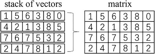
FIGURE 1. Illustration of stacking 4 vectors of (6) into a single matrix (4, 6).

In computer science, the stack operation generally converts the list of tensors having the same shape into a very compact form that is memory efficient. For example, in Matlab, for a certain problem which requires going through all the elements, transforming it into matrices production is much more efficient than using a for-loop operation for the multiplication of row vectors.

For modern machine learning or deep learning, the feeding input data are always encoded as tensors. To deal with thousands of inputs, those tensors are stacked together and reformulated into a higher-rank tensor called a batch before passing it into the model. This type of higher-rank tensor is also referred to as stack operation in machine learning.

2.2 Basics of Tensor Networks

A tensor network {Tⁱ} is the graph factorization of very large tensors by some decomposition processes like SVD or QR. The corresponding tensor results from contracting all the auxiliary bonds of the tensor network.

$\mathcal{T}\underset{\text{contraction}}{\overset{\text{decomposition}}{\leftrightharpoons }}\left\{T^i\right\},$

where T_i represents the small local tensor in the tensor network.

A graphical representation of tensors is shown in Figure 2A. In general, a rank-k tensor has k indices. Therefore, a vector as the rank-1 has one dangling leg and a rank-3 tensor has three dangling legs, as shown in Figure 2A. The contraction between two tensors can thus be defined by contracting the same index between two arbitrary tensors. In Figure 2A, a rank-1 tensor M_k is contracted with another rank-3 tensor N_i,j,k as M_k ⋅ N_i,j,k, and it ends up with a rank-2 tensor, that is, a matrix.

FIGURE 2

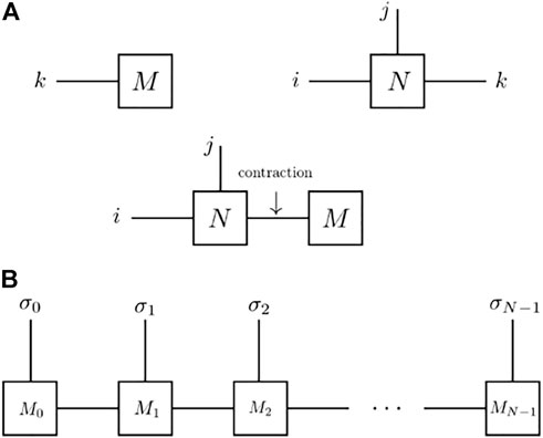
FIGURE 2. Diagrammatic representations for tensor networks: (A) Diagrammatic representations for tensors M_i and N_i,j,k, and the contraction between them M_i ⋅ N_i,j,k; (B) Diagrammatic representation for the one-dimensional tensor network MPS: M_j is the local rank-3 tensor and each is contracted via auxiliary bond dimensions (vertical solid lines); σ_j is the index for the physical dimension.

In the context of quantum physics, a many-body wave function can be represented as a one-dimensional rank-N tensor network where each leg represents the physical index for each site, as shown graphically in Figure 2B. This is usually referred to as the matrix product state (MPS). The MPS can therefore be seen as a connected array of local rank-3 tensors. Each tensor M_j has three indices: the physical index σ, and two auxiliary indices D_j and D_j+1 that are contracted and therefore, implicit. An MPS with open boundary conditions can be written as

$\left|\psi \right.⟩=\sum _{\left\{\mathit{\sigma }\right\}}\left[M_0^{{\sigma }_0}{M}_1^{{\sigma }_1}\dots M_{n-1}^{{\sigma }_{n-1}}\right]\left|{\sigma }_0,\dots ,{\sigma }_{n-1}\right.⟩.(1)$

2.3 Stack Operation for Matrix Product States

A tensor $\mathcal{T}$ can be converted to a tensor network {Tⁱ} which consists of contracted local tensors T_i via decomposition such as the tensor train method [23]. Mathematically, one could perform operations such as product, trace, contraction, splitting, and grouping on both of them.

However, the stack operation can only be directly applied to one single tensor network rather than to multiple ones separately. More precisely, we want to deal with such a problem as shown in Figure 3: given a series of tensor networks ${\{T^i\}}_{\alpha }$ with the same configuration, we want to get their stacked tensor network representation with the same physical structure and shape.

FIGURE 3

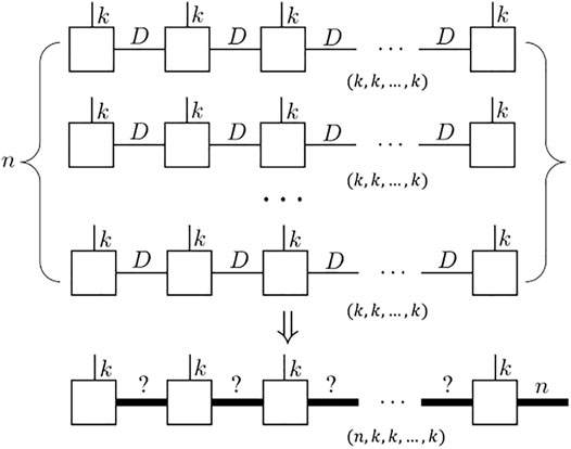
FIGURE 3. Schematics of stack operations for MPS: illustration for the n identical MPS with auxiliary bond dimension D which ends up with a new MPS with same physics dimension. One of the sites should have an extra bond dimension n to fulfill the stack dimension requirement (here we set the last site).

One direct method to realize this is to convert those tensor networks {Tⁱ} first to the corresponding tensor (k, k, … , k), and then decompose the stacked tensor (n, k, k, … , k). However, this deviates from the original intention of representing a tensor as a tensor network. It is to be noted that we use a tensor network to avoid storing or expressing the full tensor in computing, which is memory-consuming and may be prohibited in large systems. Thus, we would like to explore other approaches that can help us to efficiently establish the representation of the stacked tensor network without accessing any contraction.

We show in Figure 4 that each rank-3 tensor in the MPS is (k, nD, nD). Each matrix (nD, nD) along with the physical dimension k, is a block diagonal matrix. The i-th block (D, D) is exactly the i-th rank-3 tensor in the stack list at the same physical dimension k (so it is a matrix). There are minor differences between the start and the end of the MPS. The start tensor unit is a rank-2 matrix with a row stack for the first unit in the stack list. The end tensor is a diagonal rank-3 tensor (k, nD, n) with each diagonal D × 1 block filled by the end unit in the stack list. A full mathematical proof is given in Supplementary Appendix SA.

FIGURE 4

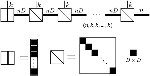
FIGURE 4. Diagram result shows the result of the “stack” operation for the MPS. It will allocate a block diagonal local rank-3 tensor: for each physical dimension, it gives a block diagonal matrix where the size of each block is a matrix (D, D). Note the first tensor unit’s block is a vector (D, ) and the last unit’s block is a matrix (D, 1)

2.4 Batch Operation for General Tensor Networks

For other types of tensor networks such as the PEPS, the unit tensor is a 4 + 1 rank tensor. The formula shown in IIC would be more complicated. We show the results here directly. For any tensor network consisting of M tensor unit

$\left\{T^i=\left(k,L_1,L_2,\dots ,L_m\right)|i=\mathrm{1,2},\dots ,M\right\}$

its n-batched tensor network version is another tensor network

$\left\{T_{\text{batch}}^i=\left(k,n{L}_1,n{L}_2,\dots ,n{L}_m\right)|i=\mathrm{1,2},\dots ,M\right\}$

with one extra index. The extra index represents the stack dimension (corresponding to the tensor stack) and is free to be added since each local tensor is block-diagonal. We only need to unsqueeze/reshape the diagonal block from (k, L₁, L₂, …) to (k, 1, L₁, L₂, …). For the MPS case, we could put it at the right end, as shown in Figure 4.

The sub-tensor (nL₁, nL₂, … , nL_m) along the physical indices for each tensor is a diagonal block tensor. For example, the j-th diagonal block is

${\left(T_{\text{batch}}^i\right)}_{k,p_1,p_2,\dots ,p_m}=T_j^i,$

where p_i is the local index for index i which takes the value from p_i ∈ [j*L_i, (j + 1)*L_i] and $T_j^i$ is the T_i of the j-th tensor network in the tensor network list ${\{T_i\}}_{\alpha }$.

Meanwhile, one unit (for example, take the N-th local tensor) should be “unsqueezed” to generate the dangling leg for the stack number indices

$T_{batch}^N=\left(k,n{L}_1,n{L}_2,\dots ,n{L}_m,n\right).$

For example, the MPS case in Section 2.3 will generate a row vector which is just the “diagonal block” form for the rank-1 tensor. The last MPS unit would get an external “leg” with the dimension N as the requirement of the batch.

3 Application

In this section, we study the potential applications of the stack of tensor networks. We apply this stack operation method to the tensor network machine learning. For a tensor network-based machine learning task, both the model and input data can be collectively represented as a tensor or tensor network. In fact, here, the model actually refers to the trainable parameters, and we would note it as the machine learning core in the following context. The forward processing to calculate a response signal y corresponding to the input x is an inner product in a linear or nonlinear function space, as the interaction between the machine learning core and the input data. The lost function is designed based on the type of task. For example, we would measure the distance between the real signal $\widehat{y}$ and the calculated signal y; for unsupervised learning, we might design the structure loss of hundreds of signals y to maximize the distance matrix. In this work, we take supervised machine learning as an example. However, such a method is flexible for any machine learning framework since it is a modeling technology. Here, by using the language from quantum physics, we denote the machine learning core as $|\mathcal{C}\rangle$ and one of the input data as |I_j = I_j(ψ)⟩. As both the core $|\mathcal{C}\rangle$ and the input |I_j⟩ are represented as tensors, this processing can be batch executed in parallel. This machine learning task can then be efficiently represented as

$\langle \mathcal{C}|\left(B,I_j\right)\rangle =\left(B,\langle \mathcal{C}|I_j\rangle \right)=\left(B,{\alpha }_j\right),(2)$

where α_j is the resulting output data, and $\left|(B,I_j)\right.⟩$ is the batch representation of B stacked tensors or a tensor network where $\left|(B,I_j)\right.⟩$ has an explicit format.

In the following sections, we consider the one-dimensional case of the MPS machine learning task as an example. As shown in Figure 5, both the core $|\mathcal{C}\rangle$ and the inputs |I_j⟩ are the MPS, and the output responsive signal α_j is the result obtained by contracting both physical bonds from the two MPS.

FIGURE 5

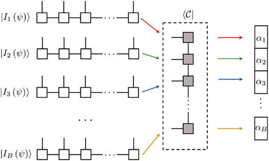
FIGURE 5. Schematics of inputting individual data as the MPS $(\left|I_j\left(\psi \right)\right.⟩)$ onto the core model $(\left.⟨\mathcal{C}\right|)$: each operation follows the arrow with the same color, and results in an outcome α_j.

In the following sections, we show that there are three ways to accomplish this machine learning task: the loop (LP) method, the batched tensor network (BTN) method, and the efficient coding (EC) method. The core MPS $|\mathcal{C}\rangle$ consists of L local tensor units with k being the dimension for all physical bonds and V being the dimension for all auxiliary bonds. Each input MPS |I_j⟩ consists of L local tensor units with k being the dimension for all physical bonds and D being the dimension for all auxiliary bonds.

3.1 Naïve Loop Method

As shown in Figure 5, for B input samples, one needs to perform B contractions to obtain B outcomes. The most obvious way to accomplish this is to perform contractions one by one. When we utilize the auto differential feature from the libraries PyTorch [25] and Tensorflow [26], the gradient information would be accumulated in every step. At the end of the loop, we can acquire the batch gradient by averaging over the sum and applying it to the gradient descent method for weight updating.

3.2 Batched Tensor Network Method

As discussed in Section 2, we can stack all the input MPS to a batched tensor network which behaves like another MPS. $\left|(B,I_j)\right.⟩=\left|I({\psi }_{\text{stack}})\right.⟩$. Assume the number of input is B, although the auxiliary bond dimension of the batched MPS $\left|(B,I_j)\right.⟩$ gets B times larger (see Figure 4), the action of the inner product

$\langle \mathcal{C}|\left(B,I_j\right)\rangle =\langle \mathcal{C}\left|I\left({\psi }_{\text{stack}}\right)\right.⟩(3)$

can now be written as one single tensor contraction, as shown in Figure 6.With the help of the format of the batched tensor network, we can now compress B times contraction into one single contraction. Our advantage is obvious: software libraries such as PyTorch and computational units such as GPU are intrinsically optimized for tensor operations, so contracting a large tensor is usually much faster than the matrix multiplication using a for-loop. As you can see in the benchmark shown in Figure 8, when using the GPU environment, the BTN method can get constant time complexity whereas the LP method is the linear function of batch size.

FIGURE 6

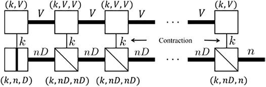
FIGURE 6. Schematics of contractions between the core MPS $\left.⟨\mathcal{C}\right|$ (upper) and the batched MPS $\left|(B,I_j)\right.⟩$ (down).

It is to be noted that we need to calculate an optimized contraction path to efficiently contract the tensor network as shown in Figure 6 whereas the LP method can simply contract the physical bond first and then sweep from left to right. When B gets larger, contracting the physical bond first in order requires storing an MPS with an auxiliary bond equal to nVB, which is quite memory consuming. Such a method would cost extra memory allocation for the block diagonal tensor. The memory increment is O(B^m), where m is the number of the auxiliary bonds. For example, the rank-3 tensor of the batched MPS will allocate a k × nB × nB memory to store only B × k × n × n valid parameters. If an auto differential action is required in the following process, the intermediate tensor required for gradient calculation will also become B times larger. Thus, although the speed is faster when the batch goes larger, the memory will gradually blow up. The BTN method is a typical “memory swap speed” method.

One possible solution is to treat the diagonal block tensor as a sparse tensor, so we only need to store the valid indices and values. Meanwhile, if we contract the physical bonds first, it will return a matrix chain whose unit is also a sparse diagonal matrix of the shape (nBV, nBV). This implies that we can block-wise compute the matrix chain so that each sparse unit performs like a compact tensor (B, nV, nV). At this juncture, it turns out that we can then use the popular coding method called efficient coding, which is widely used in modern tensor network machine learning tasks [6, 11, 14, 16, 18].

3.3 Efficient Coding

The efficient coding (EC) does the “local batch contraction” for every tensor unit calculation in the tensor network contraction.

We first batch-contract each physical index and get a tensor train consisting of batched units as shown in Figure 7, then we perform the batch contraction on all the auxiliary bonds for this batched tensor train.

FIGURE 7

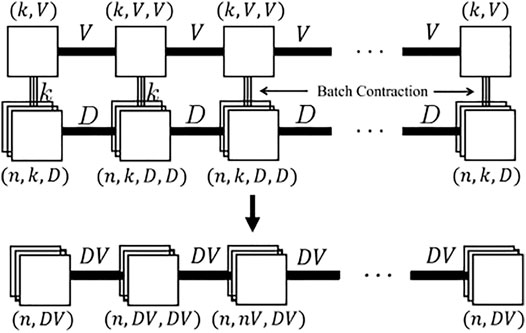
FIGURE 7. Illustration of efficient coding for the MPS. Each unit from the core MPS is batch-contracted with the input MPS (upper), and they form a batched unit as a local tensor in the resulting MPS (down).

The batch contraction is realized by the built-in function einsim which is provided in many modern scientific software libraries such as Numpy [27], PyTorch [25], and Tensorflow [26]:

$\text{einsum}(\text{’kij,Bknm}\to \text{Binjm’,core,\hspace{0.17em}batch}),(4)$

$\text{einsum}(\text{’Bij,Bjk}\to \text{Bik’,core,\hspace{0.17em}batch}).(5)$

For those without einsim, one alternative solution is to implement a highly efficient “batch matrix multiply” function. The fundamental realization of PyTorch.einsim is, in fact, the “batch matrix multiply” called PyTorch.bmm. It is to be noted that such a method is not new for tensor network machine learning, and Refs. [11, 14, 16] have already realized successful learning algorithms based on this.

The memory allocated for EC is much less than that for the BTN, which is the major reason why the BTN method is slower than EC.

Moreover, the dense BTN may require an optimized contraction path for a large batch case, while EC for the MPS would only allow contraction of the physical bond first, followed by the contraction of the auxiliary bonds as the tensor train contraction. The standard tensor train contraction method sweeps from the left-hand side of the MPS to the right. In particular, when we require all the MPS in the uniform shape, that is, all the tensor units share the same auxiliary bond dimension, we can then stack those units together (B, L, V, V) and split them by odd indices (B, L/2, V, V) or even indices (B, L/2, V, V). In doing so, we can get the half-length tensor units (B, L/2, V, V) for the next iteration by contracting the odd and even parts.

3.4 Comparison and Discussion

In Figure 8, we show the speed-up benchmark results for all three different methods introduced from Section 3.1 to Section 3.3 with respect to different batch sizes in a log —log plot. We compare the performance using different libraries in Python. We mainly test three batch contraction methods: the loop method (LP), the batch tensor network method (BTN), and the efficient coding method (EC) on the MPS batch contraction task in Figure 5. The system size is a L = 20 units MPS with each unit assigned V = 6, k = 3, and D = 1 (see Figure 7). The batch contraction task size is from 1 to 1000. Overall, EC has the best speed-up performance over other methods for almost all libraries, especially at large batch sizes. Because of the pre-processing requirement, the BTN can be slower than others in small-batch cases. The CPU is not efficient in storing and processing larger matrices or tensors, whereas the GPU is deeply optimized to deal with tensor data structures. Thus, the BTN gets similarly linear time complexity like the LP in CPU but maintains a constant time complexity in GPU. It is to be noted that the BTN will allocate tensors with (nB, nB). Thus, the larger the batch size, the larger the intermediate tensor will be. We can see that the PyTorch (CPU) gets better optimization with large tensors than NumPy. In Figures 8C, D, both BTN and EC have constant time complexity in GPU since the GPU would compress the time complexity of the matrix contraction to a constant level. It also implies that there is a close relationship between EC and BTN. As we discussed at the end of Section 3 2, the EC is another realization of the sparse matrix BTN. The redundancy memory requirement for the diagonal block tensor slows down the BTN method, but such redundancy requirement is eliminated in EC.

FIGURE 8

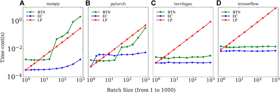
FIGURE 8. Speed-up benchmark results for different methods as a function of batch size with: (A) Numpy on CPU; (B) PyTorch on CPU; (C) PyTorch on GPU; and (D) Tensorflow on GPU. The red, blue, and green solid lines correspond to the result obtained using the loop method (LP), efficient coding (EC), and the batch tensor network method (BTN), respectively. All the panels are plotted in the log—log format. The result is tested on an Intel(R) Core(TM) i7-8700K CPU and 1080Ti GPU.

For the EC and LP methods, we contract the physical bond first, and obtain a tensor chain-like structure

$\left(B,V\right)-\left(B,V,V\right)-\left(B,V,V\right)-\cdots -\left(B,V,V\right)-\left(B,V,O\right),$

where B = 1 for the LP method and B > 1 for the EC method. Notice that we assume D = 1 here for the traditional MPS machine learning task. The memory complexity costs (L − 1) × BV² + BVO + BV as the O (B). Since the output bond is at the right-hand side, the optimal path is contracting from the left end to the right end. Here, we use the auto differential engine to automatically calculate the gradient for each unit and then, the computer records all the intermediates during the forward calculation. We therefore obtain the (B, V) batched vector calculated by a batched vector-matrix dot for the first two units

$\begin{array}{ll}\hfill & \left(B,V\right)\times \left(B,V,V\right)\to \left(B,V\right)\text{for\hspace{0.17em}the\hspace{0.17em}rest}\hfill \\ \hfill & \left(B,V\right)\times \left(B,V,O\right)\to \left(B,O\right)\text{for\hspace{0.17em}the\hspace{0.17em}last}.\hfill \end{array}$

So the memory cost for the EC and LP methods is straightforward as saving L − 1 times batched vector-matrix dot result, which is (L − 2) × BV + BO. If we apply the same contraction strategy to the BTN method, the resulted chain is

$\left(BV,\right)-\left(BV,BV\right)-\cdots -\left(BV,BV\right)-\left(BV,BO\right).$

The memory complexity then costs (L − 1) × B²V² + B²DVO + BV memory as the O (B²). Surprisingly, the intermediate cost is the same: (L − 2) × BV + BO. However, the left-right sweep path is not always the optimal path for the BTN method, as we discussed in Section 3 2. In our experiment, the memory complexity for the optimal path consumes much less than O(B²). In Figure 9, we give an example of the memory cost for increasing the batch size which takes L = 21 units of MPS with each unit assigned with V = 50, k = 3, D = 1 as the system parameters. The output O = 10 classes leg is set at the right end. The batch size increases from B = 10 to B = 1500. We also plot the B times larger curve of the EC and we simply labeled it as EC*B. We could see that although the BTN method takes more memory than the EC method, the memory complexity is much less than O(B²), which makes it an available option for machine learning. Also, for other problems which require small batches but larger auxiliary bond dimensions, the BTN will perform better than the EC method as shown in Figure 10 with a B = 10, k = 3, D = 1, O = 10 and V = 10 → 3000 MPS learning system. Contracting the auxiliary bonds first and keeping comparably smaller intermediates is a better choice when B ≪ V. This is the reason why the BTN method can allocate much less memory than the EC method for large auxiliary dimensions as shown in Figure 10.

FIGURE 9

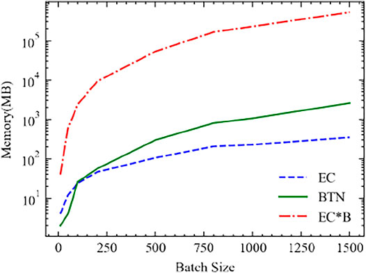
FIGURE 9. Memory required for the increasing batch size MPS machine learning problem. The system is an MPS of L = 21 units, with each unit assigned with V = 50, k = 3, D = 1, O = 10. The green curve (BTN) is the required memory for the BTN method; the blue curve (EC) is the required memory for the EC method; and the red curve (EC*B) is the B times larger curve of EC.

FIGURE 10

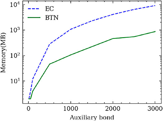
FIGURE 10. Memory required for the increasing auxiliary bond dimension MPS machine learning problem. The system is an MPS with L = 21 units, with each unit assigned with B = 10, k = 3, D = 1, O = 10. The green curve (BTN) is the required memory for the BTN method and the blue curve (EC) is the required memory for the EC method.

We also demonstrate a practice MPS machine learning task in Figure 11 and Figure 12. The dataset we used here is the MNIST handwritten digit database [28]. The machine learning task requires predicting precisely the number from 0 to 9 among the dataset. The core tensor network is a ring MPS consisting of 24 × 24 units with each unit as (V, k, V) except the last one (C, V, k, V). Here, V = 20 is the bond dimension, k = 2 is the physics bond dimension, and C = 10 is the number of classes. The bond dimension of the input tensor network is D = 1. We use the ring MPS as it is easier to train than the open boundary MPS. Figure 12 shows the valid accuracy versus time. The valid accuracy is measured after each epoch and only plots five epochs since the model gets over-fitting later. Each epoch will swap the whole dataset once. The best valid accuracy for this setup is around 92%, whereas the state-of-the-art MPS machine learning task [16] can reach 99% with a large bond .

FIGURE 11

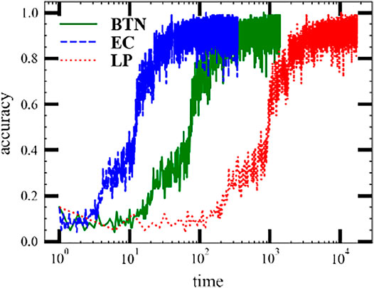
FIGURE 11. Evaluation of the train accuracy of MPS machine learning tasks on the MNIST dataset using three batch contraction methods: (red solid curve) the batch tensor network method (BTN); (green dashed curve) the efficient coding; and (blue dotted curve) the loop method (LP).

FIGURE 12

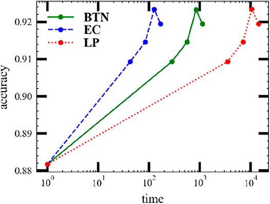
FIGURE 12. Evaluation of the valid accuracy of MPS machine learning tasks on the MNIST dataset using three batch contraction methods: (red solid curve) the batch tensor network method (BTN); (green dashed curve) the efficient coding; and (blue dotted curve) the loop method (LP).

The result is tested on an Intel(R) Core(TM) i7 − 8700K CPU and 1080Ti GPU and is shown in Figure 11. The optimizer we used here is Adadelta [28] with the learning rate lr = 0.001. The batch size is 100. The random seed is 1. The test environment is PyTorch. The x-axis shown in Figure 11 is the time cost. It is to be noted that these three methods are the only different approaches to realize the batch contraction so that they will not influence the contraction result. That is why these three curves shown in Figure 11 are exactly the same. The EC method is the best choice for tensor network machine learning. The LP method is the most inefficient method, which would cost 1 hour to traverse the dataset while EC only requires 60 s and BTN takes 300 s.

4 Conclusion

We have investigated the stack realization of the tensor network as the spread concept of the stack operation for tensors. The resulting stacked/batched tensor network consists of block-diagonal local tensors with larger bonds. We connected this method to the efficient coding batch contraction technique which is widely used in tensor network machine learning. An MPS machine learning task has been used as an example to validate its function and benchmark the performance for different batch sizes, different numerical libraries, and different chips. Our algorithm provides an alternative way of realizing fast tensor network machine learning in GPU and other advanced chips. All the codes used in this work are available at [29].

Several possible future directions may be of significant interest. Our work reveals an intrinsic connection between the block-diagonal tensor network units and the batched contraction scheme, which is potentially useful for helping researchers realize faster tensor network implementation with the block-diagonal design like [17]. Secondly, our algorithm comes without performing SVD to the stacked tensor network; it would be great to define a batch SVD and check its performance and error when truncating the singular values for a larger data size. Thirdly, the efficient coding method requires the contraction of the physical dimensions first. However, the batch method provides the possibility to start contractions in other dimensions first, which may be useful for the contraction on a two-dimensional PEPS or through the tensor renormalization group method [30–32]. Finally, the BTN method takes advantage of compressing thousands of contractions into one contracting graph. From the hardware design perspective, with a specially designed platform optimized for tensor network contraction, the BTN method may intrinsically accelerate the tensor network machine learning or any task involving a stacked tensor network. Meanwhile, the tensor network states in many-body quantum physics have a non-trivial relationship with the quantum circuits. So the idea of representing several tensors contracting into one single contraction also provides the possibility of efficiently computing on NISQ-era quantum computers.

Data Availability Statement

The datasets presented in this study can be found in online repositories. The names of the repository/repositories and accession number(s) can be found at: https://github.com/veya2ztn/Stack_of_Tensor_Network.

Author Contributions

LKA supervised the project, participated in the discussion, and edited the manuscript. TZ initiated the project, developed most of the codebase, proved the theory, ran experiments, and wrote most of the manuscript. TC participated in the discussion, assisted in proving the theory, and wrote parts of the manuscript. BY participated in the discussion and edited the manuscript. EPL participated in the discussion and funded the project.

Funding

This work was supported by US Office of Naval Research Global (N62909-19-1-2047) and SUTD-ZJU Visiting Professor (VP 201303).

Conflict of Interest

The authors declare that the research was conducted in the absence of any commercial or financial relationships that could be construed as a potential conflict of interest.

Publisher’s Note

All claims expressed in this article are solely those of the authors and do not necessarily represent those of their affiliated organizations, or those of the publisher, the editors, and the reviewers. Any product that may be evaluated in this article, or claim that may be made by its manufacturer, is not guaranteed or endorsed by the publisher.

Acknowledgments

TZ acknowledges the support of Singapore Ministry of Education PhD Research Scholarship.

Supplementary Material

The Supplementary Material for this article can be found online at: https://www.frontiersin.org/articles/10.3389/fphy.2022.906399/full#supplementary-material

References

1. Jouppi NP, Young C, Patil N, Patterson D, Agrawal G, Bajwa R, et al. In-Datacenter Performance Analysis of a Tensor Processing Unit. SIGARCH Comput Archit News (2017) 45:1–12. doi:10.1145/3140659.3080246

CrossRef Full Text | Google Scholar

2. Verstraete F, Murg V, Cirac JI. Matrix Product States, Projected Entangled Pair States, and Variational Renormalization Group Methods for Quantum Spin Systems. Adv Phys (2008) 57:143–224. doi:10.1080/14789940801912366

CrossRef Full Text | Google Scholar

3. Orús R. A Practical Introduction to Tensor Networks: Matrix Product States and Projected Entangled Pair States. Ann Phys (2014) 349:117–58. doi:10.1016/j.aop.2014.06.013

CrossRef Full Text | Google Scholar

4. Orús R. Tensor Networks for Complex Quantum Systems. Nat Rev Phys (2019) 1:538–50. doi:10.1038/s42254-019-0086-7

CrossRef Full Text | Google Scholar

5. Cirac JI, Pérez-García D, Schuch N, Verstraete F. Rev. Mod. Phys., 93 (2021). p. 045003. doi:10.1103/revmodphys.93.045003

CrossRef Full Text | Google Scholar

6. Stoudenmire E, Schwab DJ. In: D Lee, M Sugiyama, U Luxburg, I Guyon, and R Garnett, editors. Advances in Neural Information Processing Systems, 29. Curran Associates, Inc. (2016).

Google Scholar

7. Gao X, Duan L-M. Efficient Representation of Quantum many-body States with Deep Neural Networks. Nat Commun (2017) 8:662. doi:10.1038/s41467-017-00705-2

PubMed Abstract | CrossRef Full Text | Google Scholar

8. Deng D-L, Li X, Das Sarma S. Phys Rev X (2017) 7:021021. doi:10.1103/physrevx.7.021021

CrossRef Full Text

9. Stoudenmire EM. Learning Relevant Features of Data with Multi-Scale Tensor Networks. Quan Sci. Technol. (2018) 3:034003. doi:10.1088/2058-9565/aaba1a

CrossRef Full Text | Google Scholar

10. Chen J, Cheng S, Xie H, Wang L, Xiang T. Phys Rev B (2018) 97:085104. doi:10.1103/physrevb.97.085104

CrossRef Full Text

11. Han Z-Y, Wang J, Fan H, Wang L, Zhang P. Phys Rev X (2018) 8:031012. doi:10.1103/physrevx.8.031012

CrossRef Full Text

12. Glasser I, Pancotti N, Cirac JI. From Probabilistic Graphical Models to Generalized Tensor Networks for Supervised Learning (2019). arXiv:1806.05964 [quant-ph].

Google Scholar

13. Liu D, Ran S-J, Wittek P, Peng C, García RB, Su G, et al. Machine Learning by Unitary Tensor Network of Hierarchical Tree Structure. New J Phys (2019) 21:073059. doi:10.1088/1367-2630/ab31ef

CrossRef Full Text | Google Scholar

14. Efthymiou S, Hidary J, Leichenauer S. Tensornetwork for Machine Learning (2019). arXiv:1906.06329 [cs.LG].

Google Scholar

15. Roberts C, Milsted A, Ganahl M, Zalcman A, Fontaine B, Zou Y, et al. Tensornetwork. A library for physics and machine learning (2019). arXiv:1905.01330 [physics.comp-ph].

Google Scholar

16. Cheng S, Wang L, Zhang P. Supervised Learning with Projected Entangled Pair States. Phys Rev B (2021) 103:125117. doi:10.1103/physrevb.103.125117

CrossRef Full Text | Google Scholar

17. Vieijra T, Vanderstraeten L, Verstraete F. Generative Modeling with Projected Entangled-Pair States (2022). arXiv:2202.08177 [quant-ph].

Google Scholar

18. Cheng S, Wang L, Xiang T, Zhang P. Tree Tensor Networks for Generative Modeling. Phys Rev B (2019) 99:155131. doi:10.1103/physrevb.99.155131

CrossRef Full Text | Google Scholar

19. Novikov A, Podoprikhin D, Osokin A, Vetrov DP. In: C Cortes, N Lawrence, D Lee, M Sugiyama, and R Garnett, editors. Advances in Neural Information Processing Systems, 28. Curran Associates, Inc. (2015).

Google Scholar

20. Guo C, Jie Z, Lu W, Poletti D. Phys Rev E (2018) 98:042114. doi:10.1103/physreve.98.042114

CrossRef Full Text

21. Weichselbaum A. Non-abelian Symmetries in Tensor Networks: A Quantum Symmetry Space Approach. Ann Phys (2012) 327:2972–3047. doi:10.1016/j.aop.2012.07.009

CrossRef Full Text | Google Scholar

22. Hong R, Xiao Y-X, Hu J, Ji A-C, Ran S-J. Functional Tensor Network Solving many-body Schrödinger Equation (2022).

Google Scholar

23. Oseledets IV. Tensor-Train Decomposition. SIAM J Sci Comput (2011) 33:2295–317. doi:10.1137/090752286

CrossRef Full Text | Google Scholar

24. Paszke A, Gross S, Massa F, Lerer A, Bradbury J, Chanan G, et al. In: H Wallach, H Larochelle, A Beygelzimer, F d'Alché-Buc, E Fox, and R Garnett, editors. Advances in Neural Information Processing Systems 32. Curran Associates, Inc. (2019). p. 8024–35.

Google Scholar

25. Abadi M, Agarwal A, Barham P, Brevdo E, Chen Z, Citro C, et al. TensorFlow: Large-Scale Machine Learning on Heterogeneous Systems (2015). software available from tensorflow.org.

Google Scholar

26. Harris CR, Millman KJ, van der Walt SJ, Gommers R, Virtanen P, Cournapeau D, et al. Array Programming with NumPy. Nature (2020) 585:357–62. doi:10.1038/s41586-020-2649-2

PubMed Abstract | CrossRef Full Text | Google Scholar

27. LeCun Y, Cortes C, Burges CJ. Mnist Handwritten Digit Database (1998).

Google Scholar

28. Zeiler MD. Adadelta: An Adaptive Learning Rate Method (2012). arXiv:1212.5701 [cs.LG].

Google Scholar

29.veya2ztn Stack_of_Tensor_Network (2022) Available at: https://github.com/veya2ztn/Stack_of_Tensor_Network.

Google Scholar

30. Levin M, Nave CP. Tensor Renormalization Group Approach to Two-Dimensional Classical Lattice Models. Phys Rev Lett (2007) 99:120601. doi:10.1103/physrevlett.99.120601

PubMed Abstract | CrossRef Full Text | Google Scholar

31. Gu Z-C, Levin M, Wen X-G. Tensor-entanglement Renormalization Group Approach as a Unified Method for Symmetry Breaking and Topological Phase Transitions. Phys Rev B (2008) 78:205116. doi:10.1103/physrevb.78.205116

CrossRef Full Text | Google Scholar

32. Evenbly G, Vidal G. Tensor Network Renormalization. Phys Rev Lett (2015) 115:180405. doi:10.1103/physrevlett.115.180405

PubMed Abstract | CrossRef Full Text | Google Scholar